


University: Dr. A.P.J. Abdul Kalam Technical University (AKTU)
Programme: B.Tech First Year, Semester I
Course Code: AAS103D
Stream: CSE
Unit: V – Introduction to Vector Space
Notation: [[a,b],[c,d]] denotes a matrix with rows (a,b) and (c,d). Superscript ᵀ denotes transpose, † denotes conjugate transpose, and a tuple followed by ᵀ represents a column vector.
Unit V Introduction
A vector space is a collection in which addition and scalar multiplication obey precise rules. Its elements may be arrows, data records, matrices, polynomials or signals. A basis describes every element using independent building blocks.
This unit develops fields, vector spaces and their basic properties, subspaces, linear dependence and independence, basis and dimension. Applications explain engineering data modelling and compression, signal representation and noise reduction.
Complete Syllabus Map
| Topic | PDF Pages |
|---|---|
| Fields and scalar arithmetic | 2–3 |
| Vector spaces and basic properties | 4–11 |
| Subspaces and their construction | 12–19 |
| Span, dependence and independence | 20–28 |
| Basis, coordinates and dimension | 29–38 |
| Inner products and model fitting | 39–42 |
| Data, compression, signals and noise | 43–50 |
| Solved problems and revision | 51–56 |
Main Connection
A basis changes a long description into a set of coefficients. Exact reconstruction needs a spanning basis; compression may deliberately discard some directions.
Essential Notation
| Symbol | Meaning |
|---|---|
| F | Scalar field |
| V, W | Vector space and subspace |
| span(S) | All finite linear combinations of S |
| dim V | Number of vectors in a basis |
| [v]_B | Coordinates in the ordered basis B |
| ker A | Solutions of Ax=0 |
| col A | Span of the columns of A |
| Q | Matrix with orthonormal columns |
| r=x−x̂ | Reconstruction residual |
Unless stated otherwise, vectors are columns over the real field. A vector space always has a specified scalar field and specified operations.
Working Method
- Identify the elements, scalars and operations.
- Test closure before using algebraic rules.
- Use zero and closure to test a subspace.
- Turn dependence into a homogeneous system.
- Prove both spanning and independence for a basis.
- State the scalar field when giving dimension.
- Check reconstructions and discarded information.
Inner products, orthogonal projections and least squares are supporting tools for the syllabus applications. All engineering and signal data here are explicitly defined teaching examples.
1. What Is a Field?
A field F is a set with addition and multiplication. Addition is associative and commutative, has an identity 0, and every element has an additive inverse. Multiplication is associative and commutative, has an identity 1≠0, and every nonzero element has a multiplicative inverse. Multiplication distributes over addition.
Both operations are closed: adding or multiplying two field elements stays in the field. Division means multiplication by the inverse, so division by zero is excluded.
a(b+c)=ab+ac
a≠0 ⇒ aa⁻¹=1
Familiar Fields
The rational numbers Q, real numbers R and complex numbers C are fields under their ordinary operations. Negative values are allowed, and nonzero elements have inverses inside the same set.

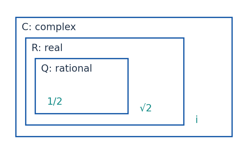
Worked Example 5.1 – Integers Fail
The integers Z have addition and multiplication, but 2 has no integer multiplicative inverse: 1/2 is not an integer. Therefore Z is not a field with the usual operations.
Positive real numbers also fail under ordinary addition because there is no additive identity 0 in the set and no additive inverse for 1.
Worked Example 5.2 – Complex Inverse
For z=1+i, multiply numerator and denominator by 1−i:
1/(1+i) = (1−i)/[(1+i)(1−i)] = (1−i)/2
The result remains complex, and multiplication by 1+i gives 1. The inverse is not the complex conjugate alone; the denominator is essential unless the modulus is 1.
Why Fields Matter
Coefficients in a linear combination must be scalars from one field. Solving for a coefficient may require division by a nonzero scalar. A field guarantees that this operation remains valid.
Quick Distinction
A vector space may contain matrices, but its scalars still come from a field. Arbitrary square matrices do not form a scalar field under matrix multiplication.
2. A Finite Field: F₂
The binary field F₂ consists of 0 and 1. Addition and multiplication are performed modulo 2. Thus 1+1=0, and 1 is its own nonzero multiplicative inverse.
| + | 0 | 1 |
|---|---|---|
| 0 | 0 | 1 |
| 1 | 1 | 0 |
| × | 0 | 1 |
|---|---|---|
| 0 | 0 | 0 |
| 1 | 0 | 1 |
There are no other elements to check. The ordinary algebraic laws survive reduction modulo 2. Subtraction equals addition because −1=1 in this field.
Worked Example 5.3 – Binary Combination
For u=(1,0,1) and v=(0,1,1), their sum in F₂³ is (1,1,0). The last component is 1+1=0, not 2.
u+v=(1,1,0)ᵀ
u+u=0
Not Every Modular System Is a Field
Modulo p arithmetic is a field when p is prime. A composite modulus can have nonzero elements whose product is zero, preventing inverses.
Worked Example 5.4 – Modulo 4 Fails
Modulo 4, 2≠0 but 2×2=0. No element multiplied by 2 gives 1 modulo 4. Hence the residue system modulo 4 is not a field.
This does not mean fields with four elements are impossible. A field with four elements exists with different construction and operations; it is not ordinary integer arithmetic modulo 4.

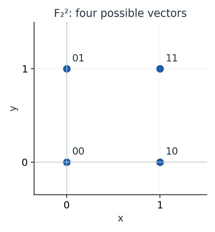
Worked Example 5.5 – Count Binary Vectors
A vector with three binary coordinates has 2³=8 possibilities. Over R, three coordinates instead give infinitely many vectors. Dimension counts independent directions, not the number of elements.
Arithmetic Rule
In binary examples, reduce each component and every equation modulo 2. Do not mix real arithmetic with binary arithmetic halfway through a calculation.
3. Vector Space: The Definition
A vector space V over F is a nonempty set with vector addition and scalar multiplication. For u,v,w in V and a,b in F, the following conditions hold.
| Addition Conditions | Scalar Conditions |
|---|---|
| u+v lies in V | av lies in V |
| u+v=v+u | a(u+v)=au+av |
| (u+v)+w=u+(v+w) | (a+b)v=av+bv |
| There is a zero vector 0 | a(bv)=(ab)v |
| Each v has inverse −v | 1v=v |
Closure is part of the definition. The zero vector belongs to V, while the scalar zero belongs to F; the same symbol is used, but their roles differ.

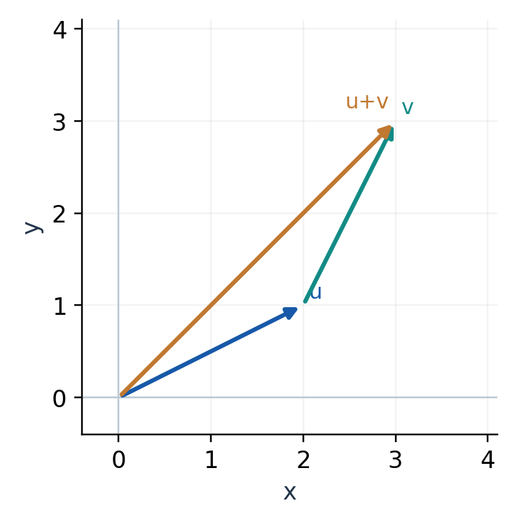
Worked Example 5.6 – Verify a Distributive Law
Take u=(1,2), v=(3,−1) and a=2. Then u+v=(4,1), so a(u+v)=(8,2). Separately au=(2,4) and av=(6,−2), whose sum is also (8,2).
This verifies one instance. To establish the law for every pair in R², use arbitrary components:
a(u₁+v₁,u₂+v₂)=(au₁+av₁,au₂+av₂)
The equality follows by distributivity in R.
Worked Example 5.7 – Find the Vector Inverse
For v=(3,−5), the additive inverse is −v=(−3,5). Their sum is (0,0), the zero vector of R². A reciprocal such as (1/3,−1/5) is not the additive inverse.
Definition Versus Examples
One successful calculation cannot prove all axioms. One failed calculation, however, is enough to disprove a claimed vector-space structure.
Answer Structure
For a standard space with componentwise operations, cite the field laws componentwise. For unusual operations, verify the actual identities and zero element instead of assuming them.
Worked Example 5.8 – Check Scalar Associativity
For v=(2,−1), a=3 and b=−2, first compute bv=(−4,2), then a(bv)=(−12,6). Direct scaling by ab=−6 gives the same result. For arbitrary entries, the equality follows from associativity of real multiplication.
The law 1v=v uses the scalar identity 1. It does not require a special multiplicative identity vector in V. Vector multiplication is not part of the vector-space definition.
4. Basic Properties from the Axioms
Several useful identities follow from the definition and need not be extra axioms. Here 0 on the left of a scalar product means scalar zero; 0 on the right means the zero vector.
0v=0
a0=0
(−1)v=−v
To prove 0v=0, write (0+0)v=0v+0v. The left side is 0v. Add the inverse of 0v to both sides to obtain the zero vector on one side and 0v on the other.
Likewise a(0+0)=a0+a0 proves a0=0. Since v+(−1)v=(1−1)v=0v=0, uniqueness of the additive inverse gives (−1)v=−v.
Cancellation
If u+w=v+w, add −w to both sides and use associativity. The result is u=v. Cancellation works because additive inverses exist.
Worked Example 5.9 – Zero Product
Suppose av=0. If a≠0, multiply by its field inverse to obtain v=a⁻¹0=0. Therefore av=0 implies either a=0 or v=0.
This property concerns scalar multiplication. It does not claim that AB=0 for matrices forces A=0 or B=0; matrix multiplication is a different operation.
Uniqueness of Zero
If 0 and z both act as additive identities, then 0+z=z because 0 is an identity, while 0+z=0 because z is an identity. Thus z=0.
Worked Example 5.10 – Solve a Vector Equation
If 3v+u=2v+w, subtract 2v and then u. The solution is v=w−u. For u=(1,−2) and w=(4,3), v=(3,5). Substitution gives both sides equal to (10,13).
Proof Trick
Start with the axiom that contains the desired expression, then cancel. Never divide by a vector; only nonzero scalars are guaranteed to have multiplicative inverses.
A vector’s negative is intrinsic to the chosen addition. Under nonstandard operations, it may differ from the ordinary componentwise negative.
Worked Example 5.11 – Uniqueness of the Negative
Suppose u+v=0 and u+w=0. Then:
v=v+0=v+(u+w)=(v+u)+w=0+w=w
Thus an additive inverse is unique. The proof uses associativity, commutativity and the identity law.
Worked Example 5.12 – Cancel a Nonzero Scalar
If 5u=5v, multiply by 1/5 to get u=v. If instead 0u=0v, no conclusion about u and v follows: both sides equal zero for every pair. A cancellation argument must explicitly exclude a zero scalar.
Worked Example 5.13 – Negating a Sum
The identity −(u+v)=(−u)+(−v) follows because adding the right-hand side to u+v gives zero after regrouping. For u=(2,1),v=(−1,3), both sides equal (−1,−4). This uses addition and inverses, without introducing vector division.
5. Real Coordinate Spaces Rⁿ
An element of Rⁿ is an ordered list of n real entries. Add lists componentwise and multiply each entry by the scalar. These operations preserve the number of components and inherit the field laws.
(u₁,…,uₙ)+(v₁,…,vₙ)=(u₁+v₁,…,uₙ+vₙ)
The zero vector is (0,…,0), and the inverse of v is obtained by negating every component. Coordinates may represent position, voltage samples, sensor channels or features.


Worked Example 5.14 – Sensor Combination
For u=(2,1,0,3) and v=(1,−1,4,2), the vector 2u−v is (3,3,−4,4). Each component is combined at its matching position.
Geometry Has Limits
R² and R³ can be drawn directly, but R⁴ has the same algebra without a faithful ordinary three-dimensional picture. A two-dimensional chart of four features is a projection, not the complete record.
Worked Example 5.15 – Missing Closure
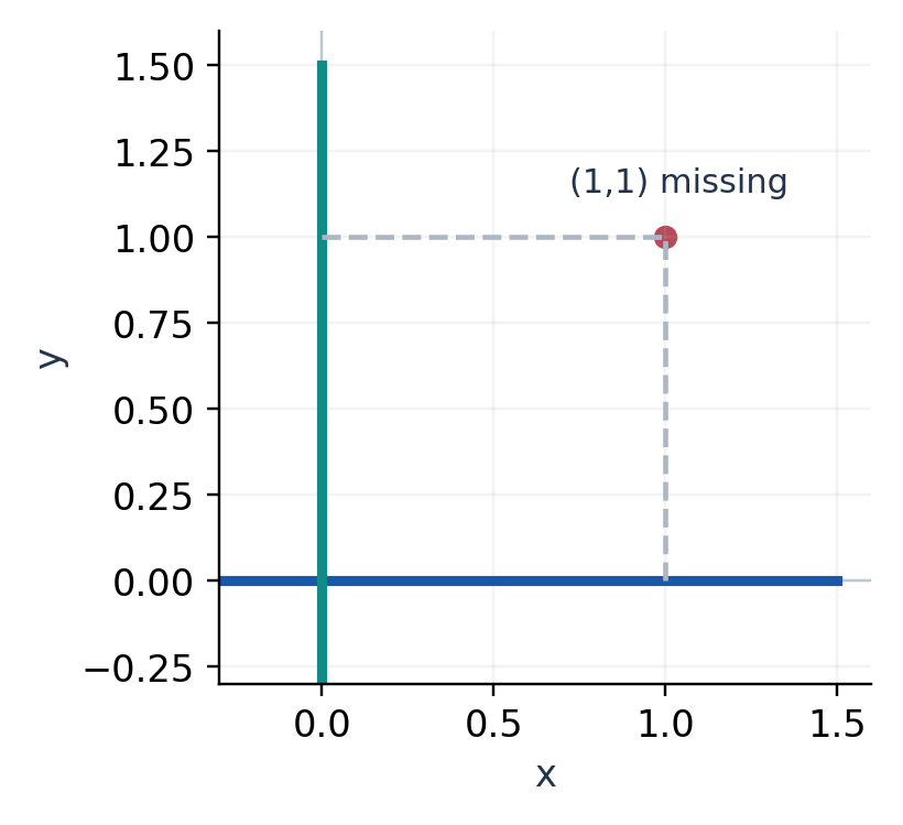
Let S contain the points of the unit circle x²+y²=1 with ordinary operations. Both (1,0) and (0,1) lie in S, but their sum (1,1) does not. Also the zero vector is missing. Hence S is not a vector space.
Units and Scaling
A mathematical vector may combine readings with different physical units, but geometric lengths can then depend strongly on units. A temperature component in kelvin and a pressure component in pascals should not automatically receive equal weight in a distance calculation.
Standardisation is a modelling choice, separate from whether Rⁿ is a vector space. It must be stated before noise reduction or compression is interpreted physically.
Exam Check
A finite list of sample records is usually not a vector space: adding two records need not produce another record in the list. Their span is a vector space.
Worked Example 5.16 – A Bounded Sensor Set
Suppose physically valid records satisfy 0≤xᵢ≤10 in every component. That bounded subset of R⁴ is not a subspace: scaling the valid record (6,0,0,0) by 2 leaves the allowed range.
The surrounding R⁴ is still a vector space. Physical feasibility and vector-space structure describe different properties. A useful physical dataset need not itself be closed under arbitrary algebraic combinations.
6. Complex Vectors and the Scalar Field
Cⁿ is a vector space over C under ordinary componentwise operations. It can also be viewed over R by restricting the allowed scalars. The elements stay the same, but independence and dimension can change.
Worked Example 5.17 – C over R
Every z=x+iy can be written x·1+y·i with real coefficients. The pair {1,i} is independent over R: a+bi=0 forces a=b=0. Thus C has dimension 2 over R.
dim_ℝ C=2
dim_ℂ C=1
Over C, the single vector 1 spans C. The pair {1,i} is dependent because i·1−1·i=0 uses valid complex coefficients that are not both zero.


Worked Example 5.18 – Complex Combination
For u=(1,i), v=(i,1), compute u+iv. Since i²=−1, iv=(−1,i), giving u+iv=(0,2i).
Now suppose au+bv=0 over C. The equations are a+ib=0 and ia+b=0. Substituting a=−ib into the second gives 2b=0; hence a=b=0. The two vectors are complex-independent and form a basis of C².
A Useful Warning
The real numbers R are not a vector space over C under ordinary multiplication: i·1=i is outside R. Closure under scalars from the stated field must hold.
Real Versus Complex Coordinates
A complex vector (z₁,z₂) has two complex coordinates or four real coordinates. For z₁=1+2i and z₂=3−i, the associated real coordinate list is (1,2,3,−1).
State the Field
Writing “dimension of C is 2” without saying “over R” leaves an essential assumption unstated. In ordinary real-vector questions, the field is R unless the question changes it.
Worked Example 5.19 – Four Real Directions in C²
The vectors (1,0),(i,0),(0,1),(0,i) form a real basis of C². For z=(a+bi,c+di), their real coefficients are exactly a,b,c,d. A zero combination forces those four real parts and imaginary parts to vanish.
Over C, only (1,0) and (0,1) are needed. The same object can therefore have two complex coordinates and four real coordinates without any contradiction.
7. Polynomial Vector Spaces
Let P₂(R) contain all real polynomials of degree at most 2, including the zero polynomial. Write p(t)=a+bt+ct². Addition and scalar multiplication act on coefficients, so results remain in P₂.
The zero polynomial has all coefficients zero. Its degree is not ordinarily defined, so it must be included explicitly rather than excluded by a careless degree statement.
p(t)=a+bt+ct² ↔ (a,b,c)ᵀ

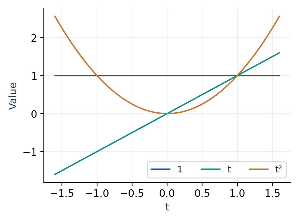
Worked Example 5.20 – Combine Polynomials
If p=1+2t−t² and q=3−t+2t², then 2p−q=−1+5t−4t². Its coefficient vector is (−1,5,−4).
Degree Exactly n Is Different
The set of polynomials of degree exactly 2 is not a vector space. Multiplying t² by zero gives the zero polynomial, which is not of degree exactly 2. Adding t² and −t² gives the same failure.
Worked Example 5.21 – Identify the Zero
The polynomial p(t)=t²−1 is zero at t=1, but it is not the zero vector in P₂. A zero vector must be the zero function for all t. Testing at one point does not establish polynomial equality.
Coefficient Comparison
Two polynomials are equal as functions on R exactly when their matching coefficients agree. This turns a polynomial identity into a system of scalar equations.
Worked Example 5.22 – Solve an Identity
If a(1+t)+b(1−t)=4+2t, then a+b=4 and a−b=2. Therefore a=3 and b=1. Substitution reconstructs 4+2t for every t.
Notation
P₂ means degree at most 2, so it contains three independent coefficient positions. Its dimension will be 3, not 2. State your convention when another text uses different polynomial-space notation.


8. Matrices as Vectors
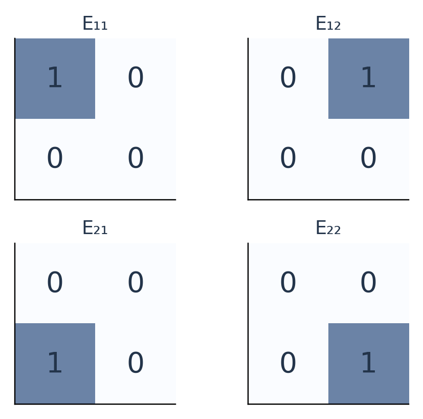
The set M₂×₂(R) of all real 2×2 matrices is a vector space with matrix addition and ordinary scalar multiplication. Here a whole matrix is one vector-space element.
A=[[a,b],[c,d]] ↔ (a,b,c,d)ᵀ
The correspondence is linear if the same entry order is always used. Four positions can vary independently. The zero vector is the all-zero matrix, and the additive inverse is −A.
Worked Example 5.23 – Matrix Combination
Let A have rows (1,2),(0,−1) and B have rows (2,0),(3,1). Then A+2B has rows (5,2),(6,1). All entries remain real and the shape stays 2×2.

Invertible Matrices Are Not a Subspace
Although each invertible 2×2 matrix belongs to M₂×₂(R), the collection of only invertible matrices is not a vector space with these operations. It excludes the zero matrix and is not closed under addition.
Worked Example 5.24 – Addition Destroys Invertibility
Both I and −I are invertible, but I+(−I)=0 is singular. A subset can be useful without being a vector subspace.
Matrix multiplication is not an operation required by the vector-space axioms. A vector space of matrices need not have multiplicative inverses.
Worked Example 5.25 – Entry Constraints
Matrices with bottom-left entry zero have the form [[a,b],[0,d]]. Their sums and scalar multiples retain that zero. The three remaining entries vary freely, suggesting dimension 3.
This is a subspace because the condition is homogeneous and linear in the entries. Conditions such as determinant equal to 1 are nonlinear and do not have the same property.
Avoid a Category Error
An identity matrix is the identity for matrix multiplication. It is not the zero vector for matrix addition. The vector-space zero here is the all-zero matrix.
9. Function and Sequence Spaces
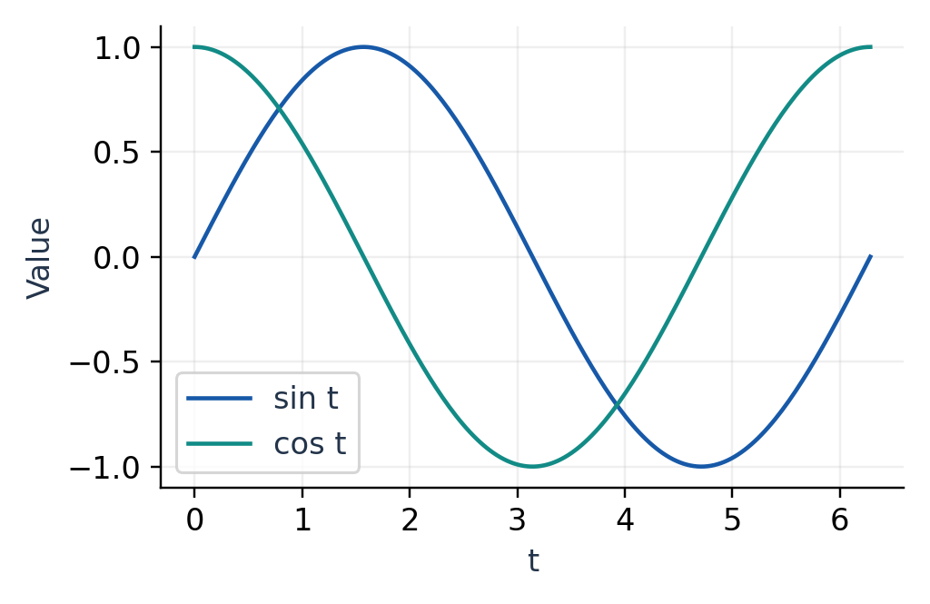
The set of all real-valued functions on a fixed domain D is a vector space under pointwise operations. Define (f+g)(t)=f(t)+g(t) and (af)(t)=a f(t). The zero vector is the function that is zero everywhere on D.
Continuous functions on an interval also form a vector space: sums and scalar multiples remain continuous. Differentiable functions form another example when the domain is fixed.
Worked Example 5.26 – A Function Combination
Take f(t)=sin t and g(t)=cos t. Then h=2f−g is the function h(t)=2 sin t−cos t, not just the number obtained at one selected time.

Finite Sampled Sequences
A real signal with N samples can be represented as x=(x₀,…,x_(N−1)) in Rᴺ. Addition combines matching time samples; scalar multiplication changes amplitude.
Worked Example 5.27 – Add Two Records
Let x=(1,0,−1,0) and y=(0,1,0,−1). Their sum is (1,1,−1,−1). The result is another four-sample record with the same sample positions.
Boundary Conditions Matter
The continuous functions satisfying f(0)=0 form a subspace. Functions satisfying f(0)=1 do not, since multiplying by zero violates the condition. A linear-looking condition with a nonzero constant may describe an affine set instead.
Infinite Dimension
The space of all real polynomials is infinite-dimensional. Any finite list has a largest degree among its members, so its linear combinations cannot generate a polynomial of higher degree.
Signal Interpretation
A finite sample vector does not uniquely specify every possible continuous signal between sample times. Reconstruction requires a signal model and sampling assumptions beyond vector-space algebra alone.
Worked Example 5.28 – A Constrained Sequence
Four-sample records satisfying x₀=x₂ and x₁=x₃ have the form (a,b,a,b). They are closed under addition and scaling, with basis (1,0,1,0),(0,1,0,1).
This is an exact repeated-pattern model, not a claim about all physical periodic signals. The sample positions are fixed, and coefficients a,b describe the two independent sample values within the model.
10. Unusual Operations: Verify Them
A set does not determine a vector space by itself. The operations matter. On the positive real numbers, define u⊕v=uv and a⊙u=uᵃ for real a. These are not the ordinary addition and multiplication used for R.
The map L(u)=ln u converts these operations into ordinary real addition and scaling:
L(u⊕v)=L(u)+L(v)
L(a⊙u)=aL(u)
Because ln maps positive reals bijectively onto R, the vector-space laws transfer. The zero vector is 1, since u⊕1=u. The additive inverse of u is 1/u.
Worked Example 5.29 – Nonstandard Sum
With u=2 and v=3, u⊕v=6. Also 0⊙2=2⁰=1, which is the zero vector for these operations. This does not contradict 0v=0.
Worked Example 5.30 – A Shifted Operation Fails
On R, suppose u⊕v=u+v+1 but scalar multiplication remains a⊙u=au. The additive identity for ⊕ would be −1. Yet 0⊙u=0 instead of −1.
More directly, a⊙(u⊕v)=a(u+v+1), while (a⊙u)⊕(a⊙v)=au+av+1. They differ when a≠1. Therefore the proposed structure fails distributivity.


Practical Test Order
- Step 1: Check both operations stay inside the set.
- Step 2: Identify the proposed zero and additive inverse.
- Step 3: Check scalar identity and both distributive laws.
- Step 4: Use a general argument for the remaining laws.
Efficient Rejection
One counterexample is decisive. You do not need to test every axiom after a single axiom fails. A proof of success, however, must cover all required laws.
Worked Example 5.31 – A Logarithmic Basis
For the positive-real space with the unusual operations, choose the element e as a basis vector. Every u>0 equals (ln u)⊙e because e^(ln u)=u. Its one real coordinate is ln u.
The vector-space sum of e² and e³ is their product e⁵, so coordinates add as 2+3=5. This illustrates why “dimension 1” refers to the chosen operations, not to the ordinary appearance of the set.
11. Subspaces: The Three-Part Test
Let V be a vector space over F. A subset W is a subspace when it is a vector space using the same operations and the same scalar field.
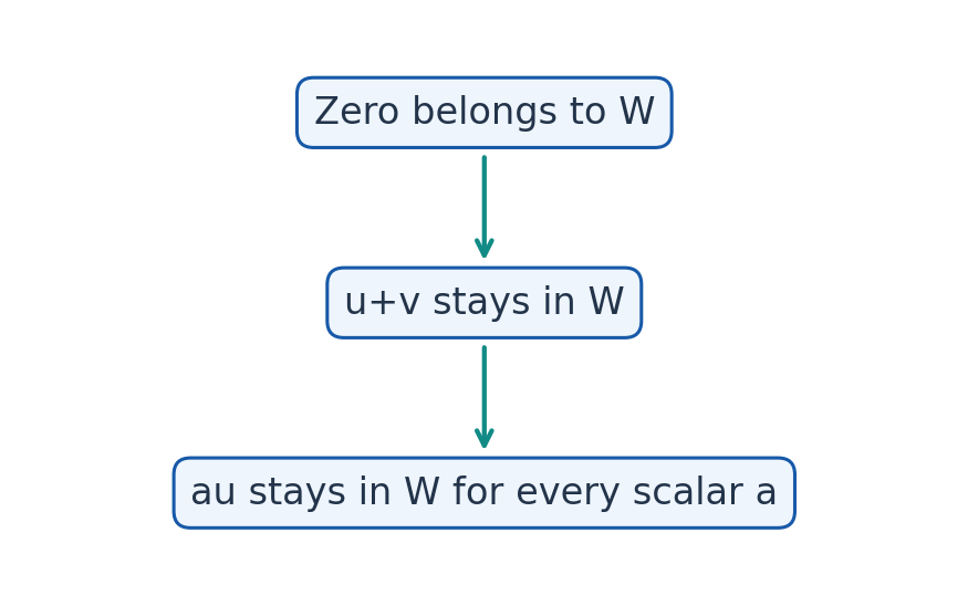
A convenient test is: W contains zero; u+v lies in W for every u,v in W; and au lies in W for every scalar a and u in W. The other axioms are inherited from V.
Equivalently, a nonempty W is a subspace if every combination au+bv remains in W. Taking a=b=0 supplies zero.
u,v∈W, a,b∈F ⇒ au+bv∈W

Worked Example 5.32 – A Coordinate Plane
Let W={(x,y,0):x,y real}. Zero lies in W. Adding (x,y,0) and (p,q,0) gives (x+p,y+q,0). Multiplying by a gives (ax,ay,0). Therefore W is a subspace of R³.
Worked Example 5.33 – A Half-Plane Fails
The set H={(x,y):y≥0} contains zero and is closed under addition. But (0,1) belongs to H and −1·(0,1)=(0,−1) does not. Closure under all scalars fails.
Why “All” Matters
Checking closure under positive scalars is insufficient for a real subspace. Negative scalars and zero are equally necessary. Checking just one pair of vectors cannot prove addition closure for the whole subset.
Short Proof Pattern
Take arbitrary members, use their defining equations, and show the resulting combination satisfies the same equations. Avoid replacing a general proof with a few convenient numerical examples.
Both {0} and V itself are subspaces. They are often called the trivial subspaces; neither should be omitted from a complete classification.
Worked Example 5.34 – A Nonempty Failure
The set W={(x,y):xy=0} contains zero and each scalar multiple of a member. Yet (1,0)+(0,1)=(1,1) is outside W. It fails only the addition part of the subspace test.
By contrast, W={(x,y):x=0 and y=0} is just {0}, which passes every part. Replacing “or” by “and” changes the subset and can change the result completely.
12. Lines Through the Origin
For a fixed nonzero vector u, the set W={tu:t real} is a line through the origin and a subspace. Adding su and tu gives (s+t)u, and multiplying tu by a gives (at)u.
Worked Example 5.35 – Parametrise a Line
The equation y=2x in R² gives (x,y)=x(1,2). Hence W=span{(1,2)}. The parameter may be negative, zero or positive.


Membership Check
A point (3,6) lies on this line because it equals 3(1,2). A point (3,5) does not: the two coordinates would demand different coefficients.
Shifted Lines Are Affine
The line y=2x+1 does not contain (0,0), so it is not a subspace. It can be written (0,1)+t(1,2): one fixed offset plus a subspace direction.
Worked Example 5.36 – Addition Test
Both (0,1) and (1,3) lie on y=2x+1. Their sum (1,4) fails, since 4≠2·1+1. The nonzero offset is counted twice when vectors are added.
A Segment Is Also Different
Even a segment on y=2x through the origin usually fails scalar closure. If it contains only t(1,2) for −1≤t≤1, then 2(1,2) is outside it.
A line subspace contains every multiple, not just a finite drawing window. The diagram displays a portion for readability.
Worked Example 5.37 – The Zero Direction
If u=0, then span{u}={0}, not a line. A line subspace needs a nonzero generating direction and has dimension 1; the zero subspace has dimension 0.
Geometric Memory
Through zero is necessary, but not sufficient: a union of two distinct lines through zero still usually fails addition closure.
Worked Example 5.38 – Two Descriptions, One Line
The lines span{(1,2)} and span{(−3,−6)} are equal, since the second generator is −3 times the first and the first is −1/3 times the second. Different generators can describe the same subspace.
To prove equality of two spans, show that each generating set lies in the other’s span. Matching one convenient point is insufficient, but matching complete generating directions is decisive.
13. Planes Defined by Homogeneous Equations
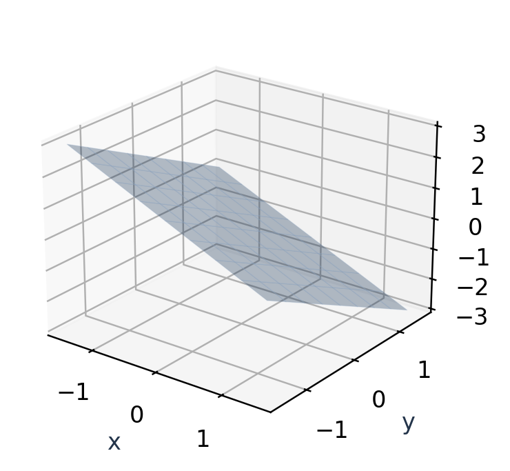
A homogeneous linear equation has zero on the right. For W={(x,y,z):x+y+z=0}, a linear combination of two solutions remains a solution because the left side is linear.
Solve for z=−x−y:
(x,y,z)ᵀ=x(1,0,−1)ᵀ+y(0,1,−1)ᵀ
The two displayed vectors span W and are independent: their first and second coordinates force both coefficients to zero in a zero combination.

Worked Example 5.39 – Plane Membership
The vector (2,−1,−1) lies in W since its entries sum to zero. Its coefficients in the displayed basis are 2 and −1. Their combination is (2,−1,−2+1)=(2,−1,−1).
The vector (1,1,1) does not lie in W, so it cannot be expressed as a combination of those two basis vectors.
Worked Example 5.40 – A Different Equation
For x−2y+z=0, set y=s and z=t. Then x=2s−t, giving s(2,1,0)+t(−1,0,1). There are two free parameters and two independent directions.
Nonzero Constants
The equation x+y+z=3 defines an affine plane, not a vector subspace, because zero is excluded. The difference of any two points on this plane lies in x+y+z=0.
Parameter Rule
Use independent free parameters and write the complete vector, including dependent coordinates. Merely saying “two parameters” is not a basis unless the generating vectors are identified and checked.
A homogeneous equation with every coefficient zero imposes no restriction: 0=0 describes the entire ambient space, not a plane of codimension one.
Worked Example 5.41 – A Normal-Vector Check
For x+y+z=0, the coefficient vector n=(1,1,1) is perpendicular to every vector in the plane because nᵀ(x,y,z)=0. Both basis vectors have zero dot product with n.
The normal is not a direction lying in the plane: nᵀn=3≠0. Confusing a plane’s normal vector with one of its spanning directions reverses its geometric role.
14. Nullspaces and Homogeneous Systems
For an m×n matrix A, its nullspace is ker A={x in Fⁿ:Ax=0}. It is a subspace because A(au+bv)=aAu+bAv=0 whenever Au=Av=0.
Worked Example 5.42 – Find a Nullspace
Take A with rows (1,2,−1,0) and (0,1,1,−1). The equations are x₁+2x₂−x₃=0 and x₂+x₃−x₄=0. Put x₃=s and x₄=t.
Then x₂=−s+t and x₁=3s−2t. Therefore:
x=s(3,−1,1,0)ᵀ+t(−2,1,0,1)ᵀ
Both generating vectors multiply to zero under A. Their third and fourth coordinates establish independence.
Worked Example 5.43 – Test a Claimed Solution
Choose s=1 and t=2, giving x=(−1,1,1,2). The first equation gives −1+2−1=0; the second gives 1+1−2=0.


Nonhomogeneous Systems
If Ax=b has a solution xₚ, then every solution has the form x=xₚ+z with z in ker A. Indeed A(x−xₚ)=b−b=0. Conversely A(xₚ+z)=b.
When b≠0, the solution set does not contain zero and is not a subspace. It is a translate of the nullspace if it is nonempty.
Distinguish Two Spaces
The nullspace lives in the input space Fⁿ. The column space lives in the output space Fᵐ. A rectangular matrix can give them different ambient dimensions.
A consistent homogeneous system always includes zero. It may contain only zero, or it may have infinitely many real solutions when there are free parameters.
Worked Example 5.44 – A Nonhomogeneous Translation
Use A=[1 1] and b=2. One solution is xₚ=(2,0), while ker A=span{(1,−1)}. Every solution is (2+t,−t).
Subtracting xₚ from a solution gives t(1,−1), a nullspace vector. Adding two solutions instead gives a vector whose component sum is 4. This verifies directly why the original solution set is affine rather than a subspace.
Worked Example 5.45 – Nullity Zero
For A=I₃, Ax=0 forces all three coordinates zero. The nullspace is {0}, whose basis is empty and whose dimension is 0. Three pivots leave no free input coordinate.
15. Polynomial Subspaces
Linear homogeneous restrictions on polynomial coefficients or values define subspaces. A restriction such as p(1)=0 is linear because (ap+bq)(1)=a p(1)+b q(1).
Worked Example 5.46 – Polynomials Vanishing at 1
Let W={p in P₂:p(1)=0}. Write p=a+bt+ct². The restriction a+b+c=0 gives a=−b−c.
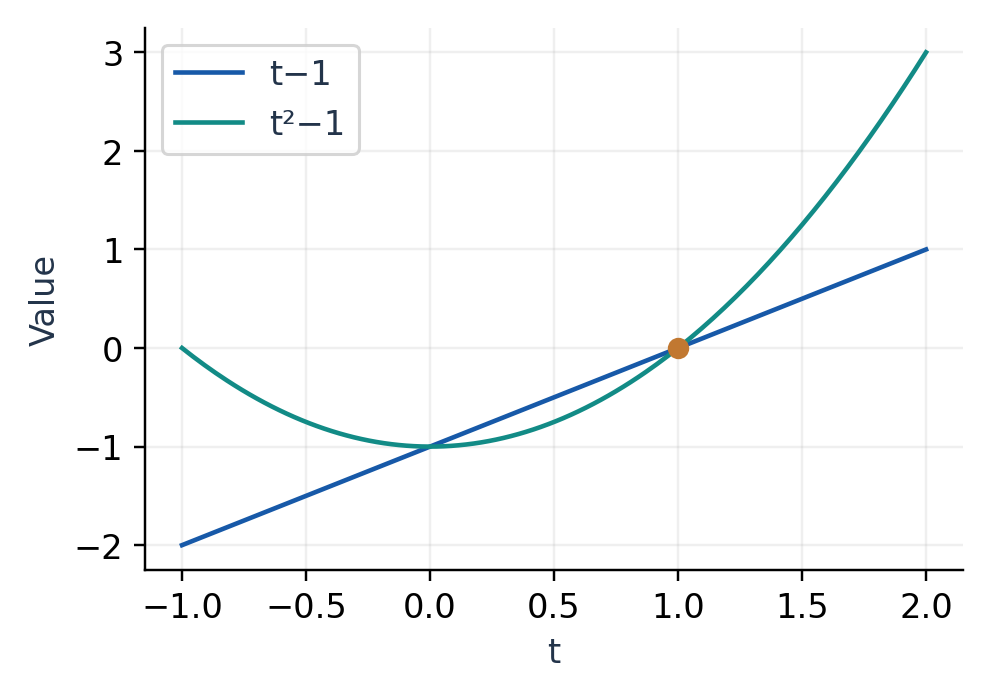
p(t)=b(t−1)+c(t²−1)
The polynomials t−1 and t²−1 span W. If α(t−1)+β(t²−1)=0, coefficient comparison gives β=0 and then α=0. Hence they form a basis, and dim W=2.

Worked Example 5.47 – An Even Subspace
The even polynomials in P₃ satisfy p(−t)=p(t). Comparing coefficients forces the t and t³ coefficients to zero. Therefore p=a+ct², with basis {1,t²} and dimension 2.
Worked Example 5.48 – A Derivative Restriction
For W={p in P₃:p′(0)=0}, write p=a+bt+ct²+dt³. Then p′(0)=b, so b=0. A basis is {1,t²,t³}, with dimension 3.
A Nonlinear Condition Fails
The set {p in P₂:p(0)p(1)=0} is not a subspace. The polynomial p=t satisfies p(0)=0, while q=1−t satisfies q(1)=0. Yet p+q=1 has neither value zero.
Translate Before Solving
Convert a polynomial restriction into equations on coefficients. Then use the same homogeneous-system methods as for coordinate vectors. A product of conditions is not the same as requiring every condition separately.
The intersection p(0)=0 and p(1)=0 is a subspace; the union of those two separate conditions need not be.
Worked Example 5.49 – Two Fixed Roots
In P₂, impose p(0)=p(1)=0. From p=a+bt+ct², the first condition gives a=0 and the second b+c=0. Therefore p=c(t²−t), and {t²−t} is a basis.
This one-dimensional space is the intersection of two larger vanishing-value subspaces. The zero polynomial remains included when c=0. Requiring exactly two distinct roots would be a different, nonclosed condition.
Worked Example 5.50 – A Nonzero Value Condition
The polynomials with p(1)=2 do not form a subspace: the zero polynomial is excluded. Their difference space is p(1)=0, so subtracting one particular polynomial, such as 2, converts the condition into a homogeneous one.
16. Matrix Subspaces
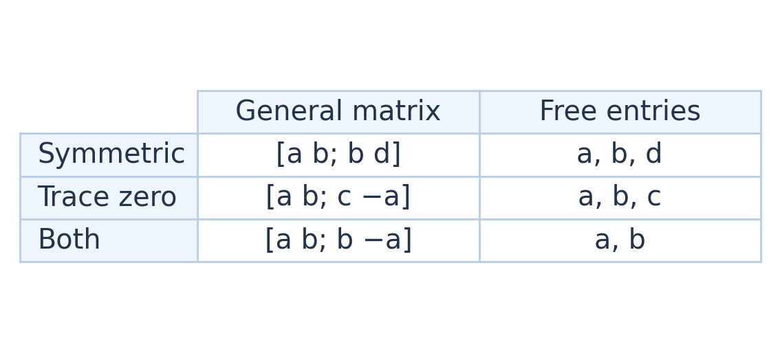
Symmetric real 2×2 matrices satisfy Aᵀ=A. They have the form [[a,b],[b,d]], and the conditions are homogeneous and linear in the entries.
A=a[[1,0],[0,0]]+b[[0,1],[1,0]]+d[[0,0],[0,1]]
The three displayed matrices form a basis. Spanning follows from the general expression; independence follows by inspecting the top-left, off-diagonal and bottom-right entries.
Worked Example 5.51 – Coordinates of a Matrix
For A=[[2,−1],[−1,3]], the coordinates in this ordered basis are (2,−1,3). The matrix has four entries, but symmetry leaves only three independent parameters.
Worked Example 5.52 – Trace-Zero Matrices
The subspace of 2×2 matrices with trace zero has form [[a,b],[c,−a]]. A basis consists of [[1,0],[0,−1]], [[0,1],[0,0]] and [[0,0],[1,0]]. Its dimension is 3.

Worked Example 5.53 – Singular Matrices Fail
Let A=diag(1,0) and B=diag(0,1). Each is singular, but A+B=I is invertible. Thus singular matrices do not form a subspace, despite containing the zero matrix and being closed under scalar multiplication.
An Intersection
Symmetric trace-zero matrices have form [[a,b],[b,−a]]. The two free parameters give a two-dimensional subspace, with basis [[1,0],[0,−1]] and [[0,1],[1,0]].
Zero Is Only the First Test
A subset containing zero may still fail addition or scalar closure. Determinant-zero conditions are nonlinear, unlike the linear entry restrictions used above.
Worked Example 5.54 – Skew-Symmetric Real Matrices
A real 2×2 skew-symmetric matrix satisfies Aᵀ=−A. Its diagonal entries obey a=−a, hence are zero over R. The remaining form is [[0,b],[−b,0]], with basis [[0,1],[−1,0]] and dimension 1.
Every real 2×2 matrix splits uniquely into symmetric and skew-symmetric parts, (A+Aᵀ)/2 and (A−Aᵀ)/2. Their intersection is zero, and dimensions 3+1 match the full matrix-space dimension 4.
17. Intersections and Sums
The intersection U∩W of subspaces is a subspace. A vector in the intersection belongs to both sets, so each linear combination remains in both.
The sum is U+W={u+w:u in U,w in W}. It is also a subspace, because combinations can be regrouped into one vector from U and one from W.
Worked Example 5.55 – Two Coordinate Planes
Let U={(x,y,0)} and W={(x,0,z)} in R³. Their intersection is {(x,0,0)}, the x-axis. Their sum is R³ because (x,y,z)=(x,y,0)+(0,0,z).


Worked Example 5.56 – Decomposition Need Not Be Unique
The vector (2,3,4) equals (2,3,0)+(0,0,4). It also equals (1,3,0)+(1,0,4). Both decompositions use U and W.
The difference comes from their common x-axis. A vector from the intersection can be moved between the two summands without changing the total.
Direct Sum
If U∩W={0}, a decomposition in U+W is unique. Suppose u₁+w₁=u₂+w₂. Then u₁−u₂=w₂−w₁ lies in the intersection, hence is zero. Thus u₁=u₂ and w₁=w₂.
Worked Example 5.57 – A Direct Decomposition
The x-axis and yz-plane in R³ meet only at zero and sum to R³. Every (x,y,z) uniquely splits as (x,0,0)+(0,y,z).
Set Symbols
U+W contains all sums; U∪W contains vectors belonging to at least one set. These are generally different. The sum is always a subspace, while the union usually is not.
Worked Example 5.58 – Count Nonunique Decompositions
For the xy- and xz-plane example, every decomposition of (2,3,4) can be written (a,3,0)+(2−a,0,4), with real a. One free parameter corresponds exactly to the one-dimensional intersection.
For the x-axis plus yz-plane, no such free transfer is possible. Their intersection contains only zero, so the first component must lie entirely in the axis summand.
18. Unions and Affine Sets
The union of two subspaces U and W is a subspace exactly when one is contained in the other. Containment makes the union equal to the larger subspace.
For the converse, suppose neither contains the other. Choose u in U but outside W and w in W but outside U. Their sum cannot belong to U, since then w=(u+w)−u would belong to U. The same reasoning excludes W.
Thus u+w is outside U∪W, and addition closure fails.

Worked Example 5.59 – A Translated Solution Set
Consider x+y=2. A particular solution is p=(2,0), and homogeneous solutions are t(1,−1). Hence every solution is p+t(1,−1).
The direction subspace has dimension 1, but the solution set itself is affine. Calling {(x,y):x+y=2} a one-dimensional vector subspace would be incorrect with ordinary operations.
Worked Example 5.60 – Difference of Solutions
Both (3,−1) and (0,2) solve x+y=2. Their difference (3,−3) solves x+y=0. Their sum (3,1) does not solve the original equation.
Data-Centering Connection
Data clustered near an affine plane can be centred by subtracting a reference mean. The centred records may then lie near a linear subspace. To reconstruct original records, add that mean back.
Useful Distinction
A nonzero offset is not another independent subspace direction. Store it separately when a compression or signal model uses centred data.
This distinction will matter when a constant signal component is removed and later restored.
Worked Example 5.61 – Centre an Affine Line
Records (1,3),(2,5),(3,7) lie on y=2x+1. Their mean is (2,5). Subtracting it gives (−1,−2),(0,0),(1,2), all in span{(1,2)}.
The centred model has one direction, but decoding needs the stored mean as well as a coefficient. Discarding the mean would reconstruct a line through the origin instead of the original affine line.
Worked Example 5.62 – A Contained Union
If U is the x-axis and W the xy-plane, then U∪W=W because U is contained in W. This union is a subspace. The containment qualification is necessary whenever stating that a union fails.
19. Linear Combinations
A linear combination of v₁,…,vₖ is any vector a₁v₁+…+aₖvₖ, where coefficients come from the scalar field. Coefficients may be zero, negative or complex when the field allows them.
Worked Example 5.63 – Form a Combination
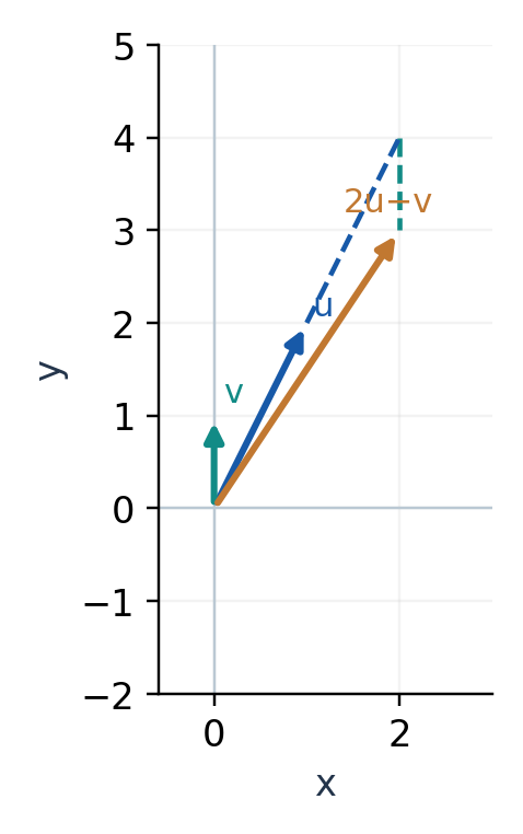
Let u=(1,2,0) and v=(0,1,1). Then 2u−v=(2,3,−1). The same coefficients apply to every component of their respective vectors.
2(1,2,0)ᵀ−(0,1,1)ᵀ=(2,3,−1)ᵀ

Reading the Equation Backwards
To decide whether b is a combination, put the generating vectors in the columns of A and solve Ac=b. The unknown vector c stores the coefficients.
Worked Example 5.64 – Recover Coefficients
For u=(1,1), v=(1,−1) and b=(5,1), solve a+b₀=5 and a−b₀=1. Thus a=3 and b₀=2, so (5,1)=3u+2v.
The temporary coefficient name b₀ distinguishes it from the target vector b. Clear notation prevents a scalar and a vector being confused.
Weighted Averages Are Restricted
A convex combination additionally requires nonnegative coefficients summing to 1. Linear combinations do not impose these restrictions. The distinction matters in data interpolation.
Worked Example 5.65 – Outside a Segment
For u=(0,0), v=(1,0), a convex combination stays on the segment 0≤x≤1. A linear combination can give (2,0) or (−3,0), so it fills the entire x-axis.
Construction Check
After finding coefficients, substitute them into the original vectors. Solving a reduced system correctly is useful, but the reconstructed target is the final check.
When generators are dependent, multiple coefficient vectors may describe the same target. The next sections explain when uniqueness is guaranteed.
20. Span: All Combinations
The span of a set S consists of all finite linear combinations of its vectors. It is a subspace: a combination of two finite combinations is another finite combination.
It is also the smallest subspace containing S. Any subspace containing each generator must contain their scalar multiples and sums, so it contains the entire span.
span{u,v}={au+bv:a,b∈F}

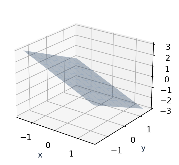
Worked Example 5.66 – One Repeated Direction
For u=(1,2,3) and v=(2,4,6), every au+bv=(a+2b)u. Their span is the same line as span{u}; two listed vectors do not guarantee dimension 2.
Worked Example 5.67 – Full R² Span
Let u=(1,1), v=(1,−1). For any target (x,y), choose a=(x+y)/2 and b=(x−y)/2. Then au+bv=(x,y). Hence these two vectors span R².
Add or Remove a Redundant Vector
If w already lies in span{u,v}, adding w does not enlarge the span. Every occurrence of w in a combination can be replaced by its combination of u and v.
Worked Example 5.68 – Redundant Generator
Let w=(2,0)=u+v for the preceding pair. Then 3u−v+2w=5u+v. Three coefficient slots were used, but only two independent directions were available.
Empty Span
By convention, span of the empty set is {0}. This makes the empty set a basis for the zero space and gives that space dimension 0.
A span contains every permitted combination, not only combinations already observed in a dataset. A drawing of finitely many sample points cannot by itself display the entire span.
Worked Example 5.69 – A Spanning-List Replacement
If w=u+2v, then span{u,v,w}=span{u,v}. Conversely, if v=(w−u)/2, then span{u,v}=span{u,w}, provided the scalar 2 is invertible in the field.
Over R this division is valid. Over F₂, the coefficient 2 equals zero, so the same expression cannot justify replacement. A seemingly harmless algebraic shortcut can depend on the scalar field.


21. Membership Through Equations
Let u=(1,0,1), v=(0,1,1). A combination au+bv=(a,b,a+b), so their span is the plane z=x+y.
Worked Example 5.70 – A Target Inside
For b=(2,3,5), the first two coordinates force a=2 and b₀=3. The third gives 2+3=5, so the target lies in the span and the coefficients are unique.
Worked Example 5.71 – A Target Outside
For c=(2,3,6), the same first two equations force coefficients 2 and 3, but the last equation would require 5=6. Thus c is outside the span.
[1,0],[0,1],[1,1]ᵀ=(2,3,6)ᵀ

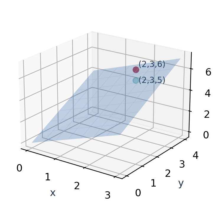
Consistency Is the Criterion
Membership asks whether Ac=b has a solution. Independence asks whether Ac=0 has only the trivial solution. These questions use related systems but answer different things.
Worked Example 5.72 – Dependent Generators
With u=(1,2) and v=(2,4), the target (3,6) gives a+2b=3. Coefficients (3,0), (1,1) and (−1,2) all work.
For target (3,7), the equations a+2b=3 and 2a+4b=7 contradict each other. The same generator set can produce a consistent nonunique system for one target and an inconsistent system for another.
Full-System Check
Do not stop after solving a convenient subset of coordinate equations. Every component must agree. An extra equation can reveal that a target lies outside the span.
No approximation has been used here. If a target lies outside a span, a best approximation is a separate problem requiring a norm or inner product.
Worked Example 5.73 – Algebraic Plane Test
For generators (1,0,1),(0,1,1), a target (p,q,r) is attainable exactly when r=p+q. The first two entries determine coefficients p,q; the third equation supplies the consistency condition.
This one equation describes the whole span without solving a fresh system for every target. It is often useful to express a subspace both parametrically and by homogeneous constraints.
22. Linear Dependence
Vectors v₁,…,vₖ are linearly dependent if some coefficients, not all zero, satisfy a₁v₁+…+aₖvₖ=0. Such a relation is called nontrivial.
If one coefficient is nonzero, solve for its vector. Thus dependence means at least one vector can be written as a combination of the others.
Worked Example 5.74 – Give a Relation
For u=(1,0,1), v=(0,1,1), w=(1,1,2), we have u+v−w=0. The coefficients (1,1,−1) are not all zero, so the set is dependent.


Worked Example 5.75 – A Zero Vector
Any set containing zero is dependent: place coefficient 1 on that vector and coefficient 0 on every other vector. The combination is zero but the coefficients are not all zero.
A singleton {v} is independent exactly when v≠0. A repeated vector also creates dependence by subtracting its two occurrences.
Pair Test
Two nonzero vectors are dependent exactly when one is a scalar multiple of the other. This simple pair test does not extend to three vectors by checking only pairs.
Worked Example 5.76 – Pairwise Independent, Jointly Dependent
The vectors (1,0), (0,1), (1,1) have no pair that is a scalar multiple. Nevertheless the first two sum to the third, so the set of all three is dependent.
Definition to Use
“Not all coefficients zero” means at least one is nonzero. It does not mean every coefficient must be nonzero. A dependence relation may leave some vectors unused.
Dependence is a property of the entire listed set and the scalar field. It does not mean that each individual vector is zero or unimportant in an application.
Worked Example 5.77 – Find All Relations
For u=(1,0,1), v=(0,1,1), w=u+v, a relation au+bv+cw=0 becomes (a+c)u+(b+c)v=0. Independence of u,v gives a=−c and b=−c.
Thus every relation is a scalar multiple of (−1,−1,1). Finding one relation proves dependence; finding this entire one-dimensional relation space describes all coefficient ambiguity.
23. Linear Independence
Vectors are independent when a zero combination forces every coefficient to be zero. The zero combination with all coefficients zero always exists; independence says it is the only one.
Worked Example 5.78 – Three Independent Vectors
Let v₁=(1,0,0), v₂=(1,1,0), v₃=(1,1,1). From av₁+bv₂+cv₃=0, the third coordinate gives c=0; the second gives b=0; the first gives a=0.
This triangular structure makes the argument immediate. The column matrix also has determinant 1, another valid check in this square example.


Independence Gives Unique Coefficients
Suppose an independent set represents the same vector in two ways: Σaᵢvᵢ=Σbᵢvᵢ. Subtracting gives Σ(aᵢ−bᵢ)vᵢ=0. Independence forces aᵢ=bᵢ for every i.
Worked Example 5.79 – Unique Reconstruction
Using the preceding three vectors, target (4,3,2) requires c=2, b+c=3 and a+b+c=4. Hence (a,b,c)=(1,1,2). No second coefficient triple can produce the same target.
Useful Inheritance Rules
Every subset of an independent set is independent. Every superset of a dependent set is dependent, since the old relation can be extended with zero coefficients.
Adding a new vector to an independent set preserves independence exactly when the new vector lies outside the old span.
Two Separate Questions
An independent set need not span the entire ambient space. For example {(1,0,0),(0,1,0)} is independent in R³, but cannot generate (0,0,1).
A basis will require both independence and spanning, not one property alone.
Worked Example 5.80 – Adding an Outside Vector
Start with e₁,e₂ in R³ and add w=(1,1,1). In ae₁+be₂+cw=0, the third entry gives c=0, then a=b=0. The enlarged set is independent.
Unlike adding e₁+e₂, the new vector has a nonzero component outside the old xy-plane. The algebraic zero-combination test captures exactly that new direction.
24. A Rectangular Independence Test
For n-component vectors v₁,…,vₖ, form A=[v₁ … vₖ]. They are independent exactly when the homogeneous system Ac=0 has only c=0, or equivalently when every column is a pivot column.
Worked Example 5.81 – Two Columns in R³
Take u=(1,2,1), v=(0,1,1). The equation au+bv=0 gives a=0 from coordinate one, then b=0 from coordinate two. Thus they are independent.
Their column matrix is 3×2. A determinant of the whole matrix is not defined, so “det A≠0” is not an appropriate test.
A=[[1,0],[2,1],[1,1]], rank A=2
Worked Example 5.82 – Four Vectors in R³
Any four vectors in R³ are dependent because a 3×4 matrix has at most three pivots. At least one coefficient is free in Ac=0, yielding a nontrivial relation.
This does not require computing the actual vectors. The same count says more than n vectors in Rⁿ must be dependent.

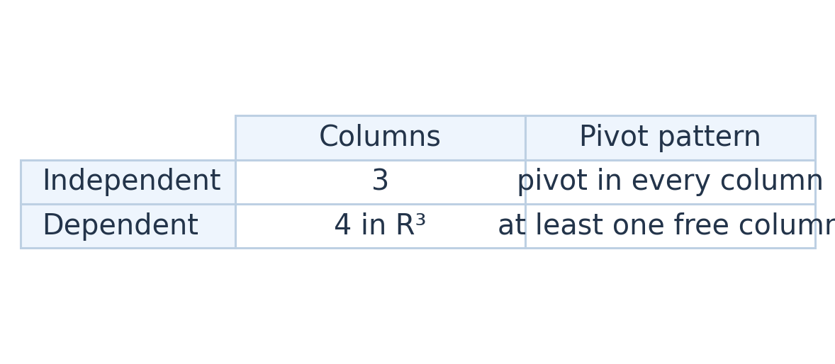
Worked Example 5.83 – Explicit Relation
For e₁,e₂,e₃ and w=(1,2,3), the relation e₁+2e₂+3e₃−w=0 exhibits the inevitable dependence.
Rank Language
Rank equals the number of independent columns. A set of k vectors in Rⁿ is independent when rank A=k, and spans Rⁿ when rank A=n. Both conditions can hold together only when k=n.
Determinant Shortcut
Use the determinant test only for a square matrix. Rank or a homogeneous-system argument works for both square and rectangular cases.
Worked Example 5.84 – Independence Versus Spanning
The columns (1,0,0),(0,1,0) have rank 2 and are independent, but their span is only the xy-plane. Adding (0,0,1) increases rank to 3 and yields a basis of R³.
Adding (2,3,0) instead keeps rank 2 and creates dependence among three columns. A rank calculation distinguishes both situations without relying on how different the vectors look.
Worked Example 5.85 – One Nonzero Column
A single column (0,0,5) has rank 1 and is independent as a one-vector set. Its span is the z-axis, not R³. A column does not need every entry nonzero to be independent.
25. Parameter-Dependent Independence
A parameter can make a direction collapse into the span of the others. Solve the general rank or determinant condition, then check exceptional values separately.
Worked Example 5.86 – Three Polynomial Vectors
In R³, take v₁=(1,1,1), v₂=(1,t,t²), v₃=(1,2,4). Their column matrix has determinant:
det([[1,1,1],[1,t,2],[1,t²,4]])=−(t−1)(t−2)
The set is independent for t≠1,2. At t=1, v₂=v₁; at t=2, v₂=v₃. Both exceptional cases visibly produce dependence.


Worked Example 5.87 – A Parameter in R²
Let u=(1,a), v=(a,1). The determinant is 1−a², so independence holds for a≠±1. At a=1 they coincide; at a=−1, v=−u.
The two exceptional values have different relations but the same conclusion. A complete answer states the independent range and explains dependence at every excluded value.
Avoid Invalid Division
If elimination creates a pivot a−1, dividing by it assumes a≠1. Branch the argument before division. Otherwise the very case that changes the answer may disappear from the calculation.
Worked Example 5.88 – One Vector Disappears
The set {(1,0),(0,a)} is independent for a≠0. At a=0 the second vector is zero, making the set dependent. Its span then drops from R² to the x-axis.
Good Final Form
Give parameter conditions explicitly, then state the span dimension in each case when asked. A determinant expression alone is not the final classification.
These examples concern exact parameters. A very small nonzero determinant can still signal numerical sensitivity in floating-point computations, even though exact independence remains true.
26. Polynomial Independence
Polynomials are vectors, so independence concerns identities valid for every input. Use coefficient comparison or a coefficient matrix in a fixed monomial order.
Worked Example 5.89 – A Nonstandard Polynomial Basis
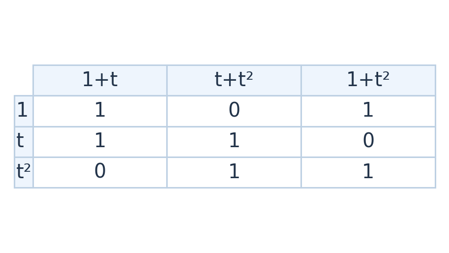
Consider p₁=1+t, p₂=t+t² and p₃=1+t². Their coefficient columns in order (1,t,t²) form:
C=[[1,0,1],[1,1,0],[0,1,1]], det C=2
Since the determinant is nonzero over R, the three polynomials are independent. As P₂ has three coefficient positions, they also span P₂.
Worked Example 5.90 – Find Coefficients
For 2+3t+t², the equations are a+c=2, a+b=3 and b+c=1. They give a=2,b=1,c=0. Hence the target is 2p₁+p₂.
Worked Example 5.91 – A Hidden Relation
The polynomials 1+t, 1−t and 2 are dependent because (1+t)+(1−t)−2=0. None is a scalar multiple of another, showing again that pairwise checks are insufficient.

Evaluating at Points
Evaluation at several points can prove independence if the resulting value matrix is nonsingular: a zero polynomial combination must give zero at those points. However, an arbitrary singular value matrix does not always prove dependence of unrestricted functions.
Worked Example 5.92 – One Point Is Insufficient
The polynomials t and t² both vanish at t=0 but are independent in P₂. Their values at that one point contain too little information to determine a polynomial identity.
Field Detail
The determinant 2 is nonzero over R. In a field of characteristic 2 it becomes zero, so the same formal coefficient columns can have different independence behaviour. Always keep the stated field.
27. Function Independence
Functions f₁,…,fₖ are independent when Σaᵢfᵢ(t)=0 for every t forces all coefficients to vanish. The domain matters: functions are compared on the whole stated domain.
Worked Example 5.93 – Sine and Cosine
Suppose a sin t+b cos t=0 for all real t. At t=0, b=0. At t=π/2, a=0. Therefore sin t and cos t are independent as functions on R.

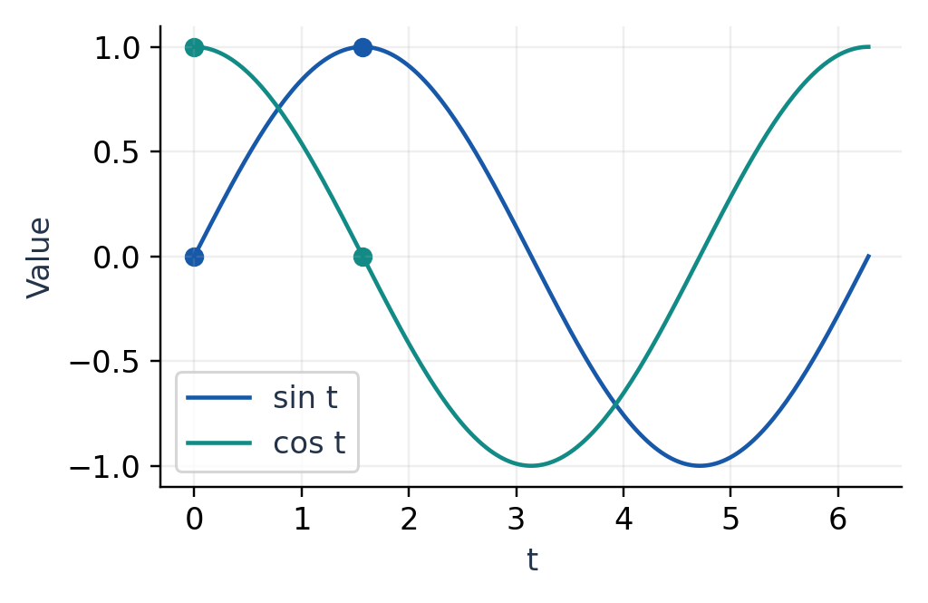
Worked Example 5.94 – A Trigonometric Relation
The functions sin²t, cos²t and 1 are dependent because sin²t+cos²t−1=0 for every real t. The relation is linear in the functions even though the functions contain squares.
Worked Example 5.95 – Exponential Independence
Suppose a+b eᵗ=0 for all t. At t=0, a+b=0. At t=ln 2, a+2b=0. Subtracting gives b=0 and then a=0. Thus {1,eᵗ} is independent.
A Restricted Domain Can Change the Answer
If the domain contains only t=0, then sin t is the zero function on that domain, so a set containing it is dependent. On a continuous interval containing both 0 and π/2, the earlier two-value proof applies.
Sample Dependence Versus Function Dependence
Two functions can be independent but yield dependent sampled records for an unfortunate choice of sample times. Sampling only at integer multiples of π makes every sine sample zero.
Method Selection
For low-degree polynomials, compare coefficients. For a small family of known functions, evaluate at informative points. A valid proof must make the coefficients unique; a plot alone does not prove independence.
Finite sampling is a linear map from functions to sample vectors. It may discard information, which is one reason signal models and sample locations must be chosen carefully.
Worked Example 5.96 – Sampling Loses a Direction
On the domain R, f(t)=t and g(t)=t² are independent. Sampling only at t=0 and t=1 gives both sample vectors (0,1), which are dependent.
The sampling map has collapsed a genuine function-space distinction. Sampling at 0,1,2 instead gives (0,1,2) and (0,1,4), which are independent because no single scalar relates their last two nonzero entries.
28. Basis: Spanning Plus Independence
A basis B of V is a set that spans V and is linearly independent. Spanning guarantees every vector can be represented; independence guarantees that the representation is unique.
For a finite ordered basis B=(v₁,…,vₙ), each v has exactly one coefficient list (c₁,…,cₙ). This list is its coordinate vector relative to B.
v=c₁v₁+…+cₙvₙ
[v]_B=(c₁,…,cₙ)ᵀ


Worked Example 5.97 – A Basis of R²
The vectors u=(1,1), v=(1,−1) are independent and span R², so they form a basis. Target (4,2) has coordinates (3,1) because 3u+v=(4,2).
Worked Example 5.98 – Spanning Without Independence
The three vectors e₁,e₂,e₁+e₂ span R² but are dependent. They form a generating set, not a basis. Removing the third vector leaves the standard basis.
Worked Example 5.99 – Independence Without Spanning
The singleton {(1,0)} is independent in R² but cannot generate (0,1). It is a basis for the x-axis, not for all of R².
Basis Order Matters for Coordinates
The sets {u,v} and {v,u} are both bases, but their ordered coordinate vectors differ. For (4,2), coordinates are (3,1) in order (u,v) and (1,3) in order (v,u).
Proof Checklist
For a proposed basis, establish that its vectors belong to the space, that they span it, and that they are independent. In a known n-dimensional space, n independent members are enough because the dimension theorem supplies spanning.
Before dimension has been established, avoid using that shortcut circularly. Direct coefficient reconstruction often proves both properties cleanly.
Worked Example 5.100 – A Basis of the Zero Space
The empty set is independent because it has no nontrivial relation, and its span is {0}. Therefore it is a basis of {0}. The singleton {0} spans the same space but is dependent, so it is not a basis.
This convention keeps the statements “basis size equals dimension” and “every independent set extends to a basis” consistent even for the zero space.
29. Standard Bases of Familiar Spaces
Rⁿ has the standard basis e₁,…,eₙ, where eᵢ has a 1 at position i and zeros elsewhere. Every vector x equals Σxᵢeᵢ, and the coordinate equations establish uniqueness.
Pₙ has standard basis {1,t,…,tⁿ}. Mₘ×ₙ has the mn single-entry matrices Eᵢⱼ. These examples connect arbitrary-looking objects to coefficient lists.
| Space over R | Standard Basis Size |
|---|---|
| Rⁿ | n |
| P₂ | 3 |
| M₂×₃ | 6 |
| Symmetric 2×2 matrices | 3 |
| Zero space | 0 |
The standard basis depends on the space and the chosen coordinate convention. There is no single standard basis shared by every vector space.
Worked Example 5.101 – A Rectangular Matrix
For A with rows (1,2,0),(−1,3,4), the standard matrix-basis coefficients are (1,2,0,−1,3,4) in row-major order. Column-major order would give a different list, so the convention must be retained.
Worked Example 5.102 – Polynomial Coordinates
For p=3−2t+5t³ in P₃, the standard coordinate vector is (3,−2,0,5). The zero coefficient of t² must be included to preserve position.


Nonstandard Bases
A basis can mix standard slots. For example {1,1+t,1+t+t²} is a basis of P₂ because its coefficient matrix is triangular with nonzero diagonal.
Dimension Versus Appearance
A 2×3 matrix is one element of a six-dimensional space. A polynomial of degree at most 3 belongs to a four-dimensional space. Count independent coefficients, not the label on the object.
Worked Example 5.103 – Symmetric 3×3 Count
A symmetric 3×3 real matrix has three independent diagonal entries and three independent off-diagonal pairs. Its dimension is therefore 6. A basis uses E₁₁,E₂₂,E₃₃ and E₁₂+E₂₁,E₁₃+E₃₁,E₂₃+E₃₂.
The general symmetric n×n count is n+n(n−1)/2=n(n+1)/2. Each paired off-diagonal basis matrix contributes two entries but only one scalar coefficient.
30. Extracting a Basis from Generators
Given a spanning list, remove vectors that are combinations of the others until an independent spanning subset remains. Row reduction makes this systematic.
Put the original vectors in columns of A, reduce A, and identify pivot-column positions. The matching columns of the original A form a basis for its column space.
Worked Example 5.104 – Select Original Columns
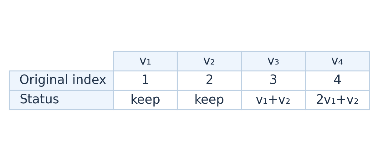
Let v₁=(1,0,1), v₂=(0,1,1), v₃=(1,1,2), v₄=(2,1,3). We have v₃=v₁+v₂ and v₄=2v₁+v₂.
rref([[1,0,1,2],[0,1,1,1],[1,1,2,3]])=[[1,0,1,2],[0,1,1,1],[0,0,0,0]]
Pivot positions 1 and 2 select {v₁,v₂}. Their span is z=x+y.

Why Not Reduced Columns?
Row operations change the actual column vectors and usually change the column space as a subset of the original output space. They preserve relations among columns, so pivot positions remain useful.
Worked Example 5.105 – A Warning
A=[[1,0],[1,0]] has column space span{(1,1)}. Its reduced form [[1,0],[0,0]] has column space span{(1,0)}. The pivot position is the same, but the geometric line is different.
Row-Space Basis
Nonzero rows of an echelon form do form a basis for the original row space, because elementary row operations replace rows by reversible combinations. Do not interchange the row-space and column-space rules.
Reconstruction Check
After selecting a basis, express every omitted generator in it. This confirms that removing the redundant vectors did not shrink the span.
A basis extracted from a finite list need not be unique. Different valid pivot orders can select different original vectors while keeping the same dimension.
Worked Example 5.106 – An Alternative Extracted Basis
For the four original columns, {v₁,v₄} also spans the same plane: v₂=v₄−2v₁ and v₃=v₄−v₁. Since v₄ is not a multiple of v₁, this pair is independent.
Thus the pivot-based answer is one valid basis, not the only possible basis. Every basis has two members even though the selected original columns may differ.
31. Extending an Independent Set
An independent list in a finite-dimensional space can be extended to a basis by adding vectors outside its current span. Each addition creates a new direction and preserves independence.
Worked Example 5.107 – Extend One Vector in R³
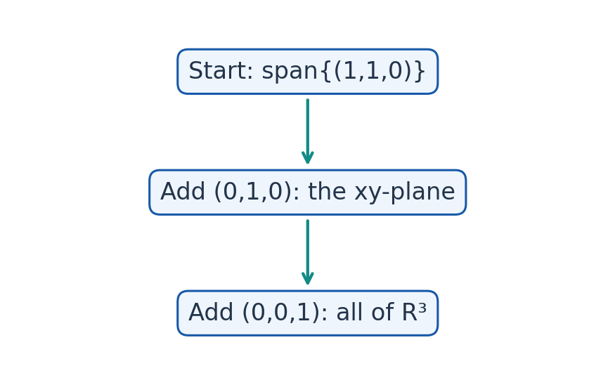
Start with u=(1,1,0). Add e₂=(0,1,0), which is not a multiple of u. Their span is the xy-plane. Add e₃=(0,0,1), which lies outside that plane.
The column matrix is triangular with diagonal entries 1,1,1, so {u,e₂,e₃} is a basis of R³.

Worked Example 5.108 – A Failed Addition
Adding w=(2,2,0) to {u} fails because w=2u. The enlarged list is dependent and its span remains the same line.
Worked Example 5.109 – Extend Polynomials
The independent pair {1,t²} in P₂ lacks the t direction. Adding t gives the basis {1,t²,t}. The order is valid even though it is not the usual monomial order.
How Many Additions?
In an n-dimensional space, an independent set of k vectors needs n−k further independent directions to become a basis. This count assumes the space’s dimension is already known.
A Constructive Algorithm
- Step 1: Keep the current independent list.
- Step 2: Examine candidate generators of the whole space.
- Step 3: Add a candidate only if it is outside the current span.
- Step 4: Stop when the list spans the space.
Do Not Add Blindly
A vector can look different but still lie in the old span. Use a membership equation or a rank increase to justify the addition.
For example, every vector (a,b,0) lies in the xy-plane; none can extend a plane basis to all of R³.
Worked Example 5.110 – Basis Extension in a Plane
Within W={z=x+y}, begin with u=(1,0,1). Add v=(0,1,1), which is in W but not in span{u}. The pair becomes a basis of W.
Adding (0,0,1) would leave W and cannot extend a basis within this particular space. A candidate must belong to the intended ambient space as well as supply a new direction.
32. Coordinates in a Basis
Coordinates depend on the chosen basis, while the vector itself remains unchanged. To find [x]_B, solve Sc=x, where S has the ordered basis vectors as columns.
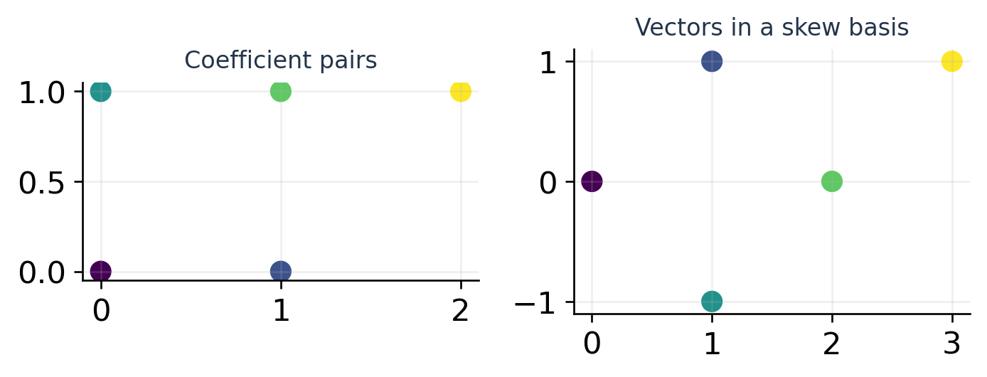
Worked Example 5.111 – A Skew Basis
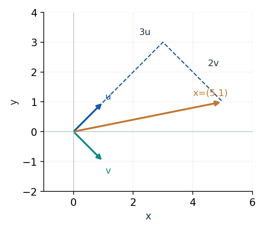
Let B=((1,1),(1,−1)) and x=(5,1). Then c₁+c₂=5 and c₁−c₂=1. Thus [x]_B=(3,2).
S=[[1,1],[1,−1]]
S⁻¹=(1/2)[[1,1],[1,−1]]
Multiplying S(3,2) gives (5,1). The numbers 3 and 2 are coefficients along basis directions; they are not the standard horizontal and vertical components.

Worked Example 5.112 – Coordinates in a Plane
For W={z=x+y} with B=((1,0,1),(0,1,1)), the vector (2,−1,1) has coordinates (2,−1). Coordinates have two entries even though the ambient vector has three.
Worked Example 5.113 – Polynomial Coordinates
In B=(1,1+t,t²), write 2+3t+4t²=a+b(1+t)+ct². Coefficients give b=3,c=4,a=−1. Thus [p]_B=(−1,3,4).
Coordinate Map
The coordinate map is linear:
[ax+by]_B=a[x]_B+b[y]_B
It is one-to-one and onto Fⁿ because the basis gives existence and uniqueness of every coefficient list.
A Common Reversal
The equation is x=S[x]_B. The inverse matrix converts standard coordinates into basis coordinates. Reversing these maps produces the wrong coefficients even when the matrix arithmetic is correct.
For a basis of a proper subspace, S may be rectangular. The coefficient system is still unique for x in that subspace, but an ordinary square inverse is not available.
Worked Example 5.114 – Coordinate Linearity
With B=((1,1),(1,−1)), let x=(5,1), y=(1,3). Their coordinates are (3,2) and (2,−1). Hence coordinates of 2x−y are (4,5).
Directly, 2x−y=(9,−1), and 4(1,1)+5(1,−1)=(9,−1). This checks that coefficient arithmetic mirrors vector arithmetic when one fixed ordered basis is used throughout.

33. Changing a Basis
Let B and C be two ordered bases of the same n-dimensional space. If their standard column matrices are S_B and S_C, then x=S_B[x]_B=S_C[x]_C.
[x]_C=S_C⁻¹S_B[x]_B
The change matrix has as its columns the B basis vectors expressed in C coordinates. Its direction must be stated: from B coefficients to C coefficients.
Worked Example 5.115 – Two Bases of R²
Take B=((1,1),(1,−1)) and C=((1,0),(1,1)). Then S_C has rows (1,1),(0,1), with inverse rows (1,−1),(0,1).
P_(C←B)=[[0,2],[1,−1]]
For [x]_B=(3,2), this gives [x]_C=(4,1). Both reconstruct x=(5,1).


Worked Example 5.116 – Reverse the Map
The inverse change matrix is [[1/2,1],[1/2,0]]. Applying it to (4,1) gives (3,2), recovering the original B coordinates.
Multiplication Order
For a third basis D, the map B to D is P_(D←C)P_(C←B). The rightmost map acts first. Basis changes compose in the same order as other linear coordinate maps.
A Quick Column Check
The first column (0,1) says the first B vector (1,1) equals 0·(1,0)+1·(1,1) in C. The second column (2,−1) says (1,−1)=2(1,0)−(1,1).
No Geometric Motion
A basis change changes the coefficient description of x. It need not rotate or move x itself. In graphics, distinguish a coordinate conversion from an active transformation of the object.
This supporting concept helps separate a compressed coefficient vector from the physical record it represents.
Worked Example 5.117 – Change the Zero Coordinates
Every linear change-of-basis matrix sends the zero coordinate vector to zero. If a proposed conversion contains a nonzero constant offset, it is an affine coordinate conversion rather than an ordinary basis change.
In the worked B-to-C example, det P=−2≠0, so the conversion is reversible. Its inverse is essential when a receiver stores coefficients in C but a calculation expects B coordinates.
34. Dimension
The dimension of a finite-dimensional vector space is the number of vectors in any basis. A fundamental theorem guarantees that all bases of the same space have the same size.
One way to understand this is the exchange principle: an independent list cannot be longer than a spanning list. Apply it to two bases in both directions to show their lengths are equal.
dim W≤dim V when W⊆V and dim V<∞
Worked Example 5.118 – A Plane’s Dimension
For W={x+y+z=0}, the basis (1,0,−1),(0,1,−1) has two vectors. Hence dim W=2, although its vectors have three ambient coordinates.


The n-Vector Shortcuts
In an n-dimensional space, any n independent vectors form a basis. Any n spanning vectors also form a basis. More than n vectors are dependent; fewer than n cannot span the whole space.
Worked Example 5.119 – Four Polynomials
In P₃, dimension is 4. If four proposed polynomials have a nonsingular 4×4 coefficient matrix, they are independent and hence a basis. A separate long spanning calculation is unnecessary once the dimension is established.
Equal Dimensions and Containment
If W is a subspace of finite-dimensional V and dim W=dim V, then W=V. A basis of W already has enough independent vectors to be a basis of V.
Worked Example 5.120 – Proper Subspace
A two-dimensional subspace of R³ is proper because its dimension is smaller than 3. However, two different two-dimensional subspaces need not contain one another; the xy-plane and xz-plane are examples.
Field Requirement
Dimension is relative to a scalar field. C² has complex dimension 2 but real dimension 4. The theorem comparing dimensions assumes the same field.
35. Rank and Nullity
For A with n columns, rank is dim(col A), and nullity is dim(ker A). Rank–nullity states:
rank A+nullity A=n
Each pivot variable corresponds to an independent output direction; each free variable contributes one independent nullspace direction. The sum equals the number of input coordinates.
Worked Example 5.121 – A 2×4 Map
For the matrix with rows (1,2,−1,0),(0,1,1,−1), there are two pivots. Rank is 2, nullity is 2, and 2+2=4 matches the four columns.
The nullspace basis is (3,−1,1,0),(−2,1,0,1), as calculated earlier. The first two original columns (1,0),(2,1) form a column-space basis.


Worked Example 5.122 – Full Column Rank
A 5×3 matrix of rank 3 has nullity 0. Its columns are independent and Ax=b has at most one solution. It cannot produce every b in R⁵ because its output span has dimension only 3.
Worked Example 5.123 – Full Row Rank
A 3×5 matrix of rank 3 has nullity 2. Every b in R³ is attainable, but each solution has two free homogeneous directions, so it is not unique.
Zero Map
For the zero m×n matrix, rank is 0 and nullity is n. All input vectors map to zero, and only the zero output can be produced.
Count the Correct Side
Rank–nullity uses the number of columns, the input dimension. The number of rows gives the output ambient dimension and may be different.
This theorem links dimension to solving systems without repeating a complete elimination argument for every question.
Worked Example 5.124 – A Map from R³ to R²
Let A have rows (1,0,1),(0,1,1). Its columns span R², so rank is 2. The kernel equation gives x₁=−x₃,x₂=−x₃, with basis (−1,−1,1) and nullity 1.
The record (1,1,−1) maps to zero despite being nonzero. Full output coverage does not imply unique input recovery when the input space has extra dimensions.
36. Dimension of a Sum
For finite-dimensional subspaces U and W:
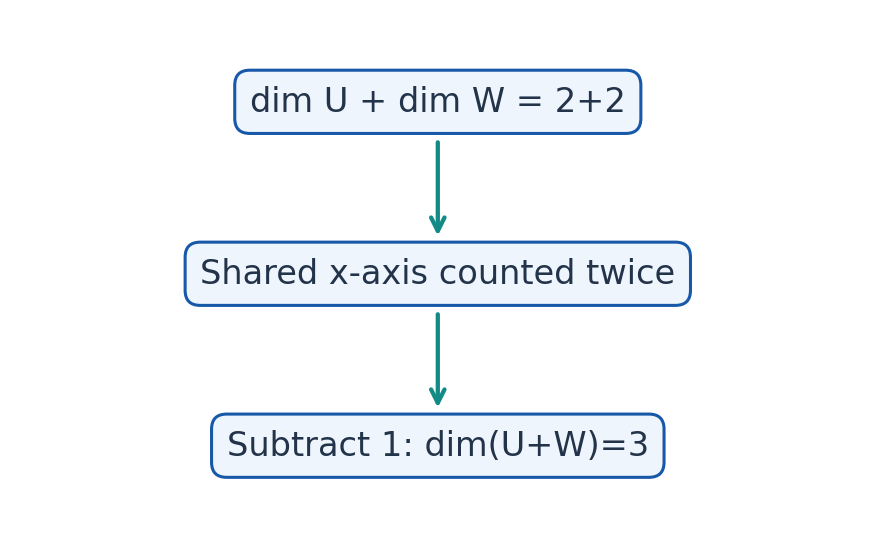
dim(U+W)=dim U+dim W−dim(U∩W)
Adding the two dimensions counts common directions twice. Subtracting the intersection dimension corrects that double count.
Worked Example 5.125 – Two Planes
The xy-plane and xz-plane each have dimension 2. Their intersection is the one-dimensional x-axis. Hence dim(U+W)=2+2−1=3, agreeing with U+W=R³.
Worked Example 5.126 – A Line Inside a Plane
If U is the x-axis and W is the xy-plane, then U∩W=U and U+W=W. The formula gives 1+2−1=2.

Worked Example 5.127 – Find an Intersection
Let U be z=0 and W be x+y+z=0 in R³. In their intersection, z=0 and x+y=0, so (x,y,z)=t(1,−1,0). The intersection has dimension 1; the sum has dimension 3.
A basis of U+W can be formed from e₁,e₂ and a W vector outside U, such as (1,0,−1). These three vectors are independent.
A Dimension Lower Bound
If U and W lie in an n-dimensional space, then:
dim(U∩W)≥dim U+dim W−n
This follows because dim(U+W)≤n.
Worked Example 5.128 – Forced Overlap
Two three-dimensional subspaces of R⁴ must intersect in dimension at least 2. They cannot meet only at zero. This conclusion follows from dimensions alone.
Direct Sum Criterion
If the intersection is {0}, then dimensions add without subtraction. Conversely, a zero intersection gives uniqueness of the sum decomposition.
A union does not obey this dimension formula in general because it may not be a vector space at all.
Worked Example 5.129 – Distinct Lines
For U=span{(1,0)} and W=span{(1,1)} in R², the intersection is zero: equality a(1,0)=b(1,1) forces b=0 and then a=0. Their sum is R², and dimensions add as 1+1=2.
If W is replaced by span{(2,0)}, the two lines coincide, their intersection has dimension 1 and their sum has dimension 1.
37. Comparing Abstract Spaces
Two finite-dimensional vector spaces over the same field with equal dimension admit a linear one-to-one correspondence. Choose ordered bases and match their coefficient lists.
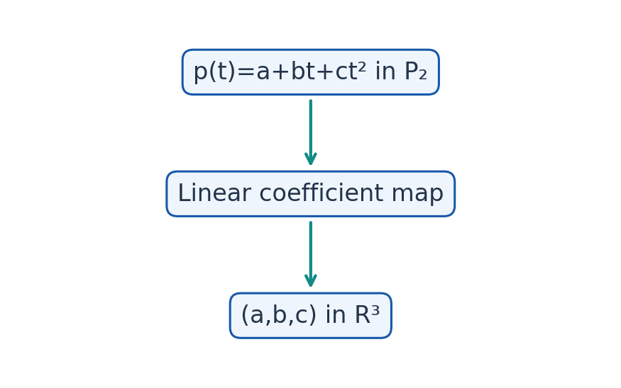
For example, P₂(R) and R³ are both three-dimensional. The map a+bt+ct²↦(a,b,c) preserves addition and real scaling, is one-to-one and reaches every real triple.
T(ap+bq)=aT(p)+bT(q)
This does not say a polynomial and an arrow are physically the same object. It says their linear structures can be represented by the same coefficient algebra.

Worked Example 5.130 – A Matrix Correspondence
Symmetric 2×2 matrices [[a,b],[b,d]] correspond linearly to (a,b,d) in R³. The inverse map inserts the middle coordinate into both off-diagonal entries.
A Metric Warning
The raw coefficient correspondence does not automatically preserve lengths or inner products. The Frobenius norm of [[a,b],[b,d]] has square a²+2b²+d², while the ordinary norm of (a,b,d) has square a²+b²+d².
Using (a,√2 b,d) instead would preserve this particular matrix norm. Linear equivalence and metric equivalence are different requirements.
Worked Example 5.131 – Dimension Mismatch
P₂ and R² cannot have a linear bijection because their dimensions are 3 and 2. A map sending a polynomial only to its values at two points must lose some information.
Engineering Interpretation
Choose coefficient coordinates that preserve the information your application needs. If distances or energies matter, specify the inner product rather than assuming every linear coordinate map preserves them.
This prepares the next tools for compression and noise filtering, where approximation quality is measured by a norm.
Worked Example 5.132 – An Evaluation Map Loses Information
Map p in P₂ to (p(0),p(1)). The polynomial t(t−1) is nonzero but maps to (0,0), so this linear map is not one-to-one.
Every target pair (a,b) is attained by p(t)=a+(b−a)t, so the map is onto R². A linear map can therefore reach every output while still discarding one independent input direction.
38. Inner Products for Applications
A vector space alone has no built-in notion of angle or closest vector. For real sample vectors, the Euclidean inner product is xᵀy=Σxᵢyᵢ. The associated norm is √(xᵀx).
Vectors are orthogonal when their inner product is zero. Nonzero orthogonal vectors are independent. An orthonormal list additionally has every vector of norm 1.
qᵢᵀqⱼ=1 if i=j, and 0 if i≠j
Worked Example 5.133 – Orthogonal Directions
Let u=(1,1) and v=(1,−1). Their dot product is 1−1=0, and each norm is √2. Dividing both by √2 produces an orthonormal basis.


Worked Example 5.134 – Orthogonal but Not Unit
For u=(2,0), v=(0,3), the vector x=(4,6) has coefficients 2 and 2. The raw dot products uᵀx=8 and vᵀx=18 are not those coefficients.
For an orthogonal basis:
cᵢ=(uᵢᵀx)/(uᵢᵀuᵢ)
For an orthonormal basis the denominator is 1.
Orthogonality Implies Independence
If Σaᵢuᵢ=0 for nonzero mutually orthogonal uᵢ, take the inner product with uⱼ. All cross terms vanish, leaving aⱼ||uⱼ||²=0. Thus aⱼ=0 for each j.
Complex Adjustment
For complex vectors, use x†y, including conjugation. The expression xᵀx may vanish for a nonzero complex vector; for x=(1,i), it equals 0, while x†x=2.
Scope
Inner products are introduced here to make the listed signal and noise applications precise. They add geometric structure to a vector space; they are not extra vector-space axioms.
Worked Example 5.135 – Distance Depends on Scaling
For x=(1,100) and y=(2,100), the Euclidean difference norm is 1. If the first component’s unit conversion multiplies it by 1000, the same physical difference has numerical norm 1000.
This is why a signal or engineering-data projection must specify component scaling. The abstract subspace is an algebraic model, while the chosen norm determines which approximation is called closest.
39. Building an Orthonormal Basis
Gram–Schmidt removes previously represented directions from an independent list, then normalises the remaining vectors. In exact arithmetic, each remainder is nonzero because the starting list is independent.
For u₁,u₂:
q₁=u₁/||u₁||
v₂=u₂−(q₁ᵀu₂)q₁
q₂=v₂/||v₂||
Worked Example 5.136 – Two Directions in R³
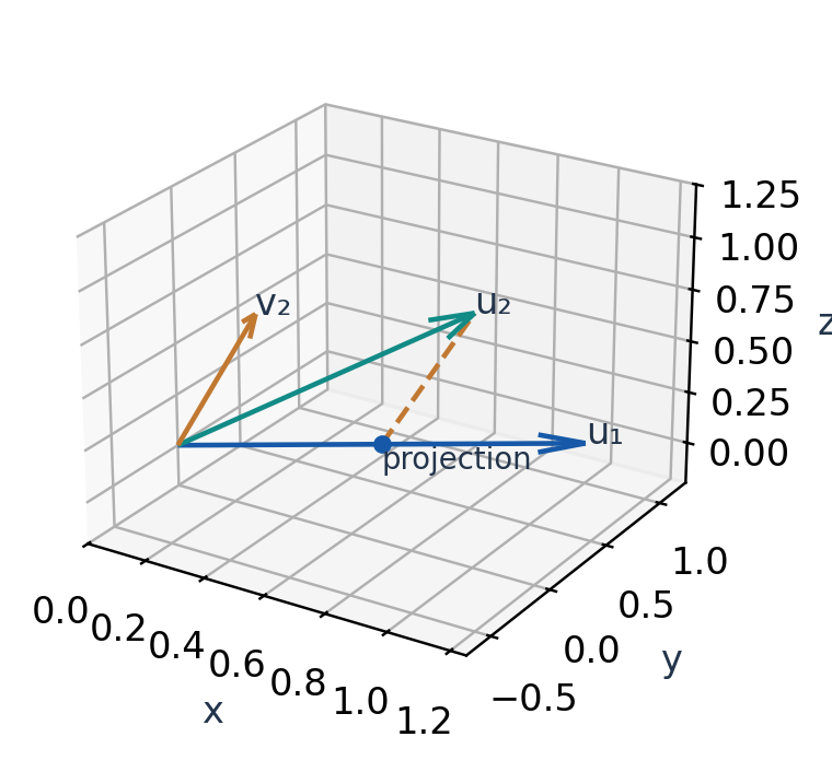
Take u₁=(1,1,0), u₂=(1,0,1). Then q₁=(1,1,0)/√2. The removed projection is (1/2,1/2,0), leaving v₂=(1/2,−1/2,1).
q₁=(1,1,0)ᵀ/√2
q₂=(1,−1,2)ᵀ/√6
Their dot product is zero and each norm is 1. They span the same plane as the original pair.

Worked Example 5.137 – Check Reconstruction
The second original vector satisfies:
u₂=(1/√2)q₁+(√6/2)q₂
Substituting gives (1/2,1/2,0)+(1/2,−1/2,1)=(1,0,1).
A Dependent Input
If u₂=2u₁, its perpendicular remainder is zero. Do not divide by its norm. The zero remainder reveals that the input direction was redundant and should be omitted.
Numerical Practice
Very small remainders can occur for nearly dependent data. Floating-point software often uses modified Gram–Schmidt or QR factorisation with a tolerance. Exact mathematical dependence and practical numerical rank are not identical questions.
Preserve the Space
Gram–Schmidt changes the basis vectors but preserves the span. It creates an orthonormal description of the same subspace rather than a new model.
This is useful when coefficients will be computed many times for compression or denoising.
Worked Example 5.138 – The Preserved Plane
The original vectors (1,1,0),(1,0,1) lie in the plane x−y−z=0. Both normalised vectors q₁ and q₂ satisfy that equation as well.
Every Gram–Schmidt subtraction uses combinations of original vectors, so the new directions remain inside the same plane. Recovering the originals from the new basis proves that the span did not shrink.
40. Projection onto a Subspace
Let Q have orthonormal columns spanning W. The orthogonal projection of x onto W is x̂=QQᵀx. Its coefficient vector is c=Qᵀx, and its residual r=x−x̂ is perpendicular to every column of Q.
Qᵀr=0
||x||²=||x̂||²+||r||²
Worked Example 5.139 – Projection onto a Line
For q=(1,1)/√2 and x=(3,1), the coefficient qᵀx=2√2. Hence x̂=(2,2), and r=(1,−1). The residual dot q is zero.
The original squared norm is 10, the retained squared norm is 8 and the residual squared norm is 2. Their sum checks exactly.

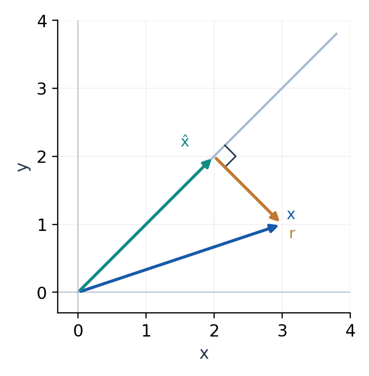
Why It Is Closest
For any w in W, x−w=r+(x̂−w), with the two terms orthogonal. Thus:
||x−w||²=||r||²+||x̂−w||²≥||r||²
Equality holds only when w=x̂.
Worked Example 5.140 – Projection Matrix
The line projection has matrix P=(1/2)[[1,1],[1,1]]. It satisfies Pᵀ=P and P²=P. Applying it twice changes nothing after the first projection.
General Independent Basis
If B has independent columns but is not orthonormal, the coefficients solve BᵀBc=Bᵀx. In real Euclidean geometry:
x̂=B(BᵀB)⁻¹Bᵀx
Using BBᵀx without orthonormal columns is generally wrong. If the columns are dependent, this inverse does not exist; first choose an independent basis or use a suitable pseudoinverse.
Exact Model
If x already belongs to W, projection reconstructs x exactly. Otherwise the residual records discarded information; it is not automatically “noise.”
Worked Example 5.141 – Nonorthonormal Projection
Use B=(2,2) as a single column and x=(3,1). Then BᵀB=8 and Bᵀx=8, giving coefficient c=1 and fitted vector (2,2).
The raw expression BBᵀx instead gives (16,16), which is not even the nearest point. Scaling a basis vector should change its coefficient inversely, leaving the projection unchanged; the normal equations achieve that.
41. Least Squares as a Model Fit
Least squares chooses model coefficients to minimise ||Bc−y||². For independent columns, the normal equations are BᵀBc=Bᵀy. The fitted record is the projection of y onto the model column space.
Worked Example 5.142 – Fit a Straight Trend
At times t=0,1,2, readings are y=(1,2,2). Use model ŷ=a+bt. The design matrix has columns (1,1,1) and (0,1,2).
[3,3],[3,5]ᵀ=(5,6)ᵀ
Solving gives a=7/6 and b=1/2. The fitted values are (7/6,5/3,13/6), and residuals y−ŷ=(−1/6,1/3,−1/6).

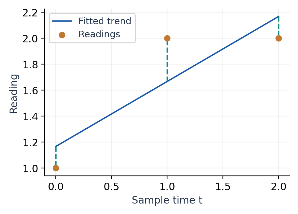
Verify Orthogonality
The residuals sum to zero: −1/6+1/3−1/6=0. Their time-weighted sum is 0+(1)(1/3)+(2)(−1/6)=0. Thus the residual is perpendicular to both model columns.
The squared residual norm is 1/36+1/9+1/36=1/6. This is the minimum among all straight-line sample records for this dataset.
Meaning of “Best”
Best here means minimum sum of squared sample errors. It does not mean the model is physically correct or best under every loss function. Outliers can strongly influence squared error.
Worked Example 5.143 – A Constant-Only Model
Restricting the model to a constant gives the mean 5/3 at all three times. Its squared error is 2/3, larger than 1/6. Adding the trend direction improves the fit but also changes what variations the model can represent.
Data Convention
Rows are sample times and columns are model directions in this example. State that convention before forming BᵀB.
Worked Example 5.144 – Compare a Candidate Line
The constant model (2,2,2) has residual (−1,0,0) and squared error 1 for the three readings. The fitted trend’s squared error 1/6 is smaller.
This comparison illustrates minimisation, while the residual orthogonality supplies the general proof against every straight-line candidate. Checking only a few alternatives cannot establish that a fit is globally least-squares.
42. Engineering Data as a Subspace Model
Suppose three sensor channels depend on two underlying quantities a and b. A simplified linear model is x=(a,b,a+b). Its records lie in W=span{(1,0,1),(0,1,1)}.
The vector x contains three readings, but only two are independently variable. The third is determined by the first two in this exact model.
Worked Example 5.145 – Encode a Valid Record
For x=(2,3,5), the two coefficients are (a,b)=(2,3). Decoding reconstructs (2,3,2+3) exactly. A stored model basis is necessary to interpret the coefficients.

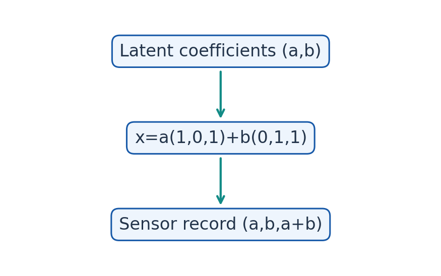
Worked Example 5.146 – An Off-Model Record
The measured record (2,3,6) violates z=x+y by 1. It cannot be represented exactly by the two-dimensional model. Simply storing the first two values reconstructs (2,3,5), leaving residual (0,0,1).
That procedure is an encoding rule, but it is not the Euclidean nearest-plane projection. The distinction matters when all three sensor readings carry comparable uncertainty.
A Modelling Workflow
- Step 1: Define component meanings and units.
- Step 2: Specify a candidate linear or centred affine model.
- Step 3: Find independent model directions.
- Step 4: Encode coefficients and reconstruct records.
- Step 5: Measure residuals against application needs.
Model Limitations
Real sensor relationships may be nonlinear, time-varying or affected by calibration drift. A vector-space model is an approximation unless physical laws or data establish exact linear dependence.
Redundancy Versus Damage
A channel is redundant only relative to the model. Removing it can discard useful fault information, even when it is predictable under normal conditions.
These considerations prevent a mathematically compact model from being mistaken for a complete description of a physical system.
43. Removing Exact Data Redundancy
Let basis columns be u=(1,0,1), v=(0,1,1), and collect several records in columns of X. If every record is a combination of u,v, write X=BC, where B=[u v] and C stores the coefficient columns.
Worked Example 5.147 – Three Records
Take coefficient columns (1,2),(2,1),(−1,3). Their decoded records are (1,2,3),(2,1,3),(−1,3,2).
B=[[1,0],[0,1],[1,1]]
C=[[1,2,−1],[2,1,3]]
The raw data matrix has nine entries. The coefficients alone have six, but storing B requires six more. For this tiny dataset, storing both costs more than the original.

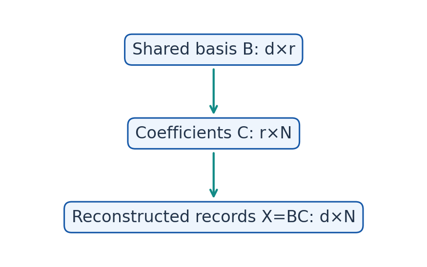
Storage Count
For d channels, r basis directions and N records, raw storage is dN numbers. A dense basis plus coefficients uses dr+rN numbers, ignoring other metadata.
Compression needs dr+rN<dN
Worked Example 5.148 – Larger Batch
For d=20,r=3,N=100, raw storage is 2000 values, while basis plus coefficients uses 60+300=360. The raw-to-model ratio is 2000/360≈5.56, before accounting for means, precision, file headers or encoding overhead.
Shared Model Assumption
This saving assumes the same basis serves all records. If each record needs a different basis, the overhead can remove the advantage.
Exact Versus Approximate
Exact low-rank data can be reconstructed without algebraic loss. Quantising stored coefficients or using an approximate learned basis can still introduce numerical loss.
A storage count in real numbers is not automatically a byte count. Precision and representation must be specified for an actual file-size comparison.
Worked Example 5.149 – When Overhead Pays Off
For d=3,r=2, dense basis-plus-coefficient storage uses 6+2N values, compared with 3N raw values. A saving requires N>6. At N=6 the counts tie; at N=10 they are 26 versus 30.
If the basis is already shared and need not be retransmitted, the coefficient payload alone uses 2N values. Report clearly which storage convention is being compared.


44. Orthonormal Transform Compression
An orthonormal basis converts a record x into coefficients c=Qᵀx. With a complete square Q, decoding x=Qc loses no information in exact arithmetic. Compression starts only when coefficients are discarded, quantised or encoded more efficiently.
For four samples, use the orthonormal directions:
q₁=(1,1,1,1)ᵀ/2
q₂=(1,1,−1,−1)ᵀ/2
q₃=(1,−1,1,−1)ᵀ/2
q₄=(1,−1,−1,1)ᵀ/2
Each has squared norm 1, and all cross-products are zero.
Worked Example 5.150 – A Compact Record
For x=(3,3,1,1), coefficients are (4,2,0,0). Thus x=4q₁+2q₂. Only two nonzero coefficients are needed once the shared basis and coefficient positions are known.

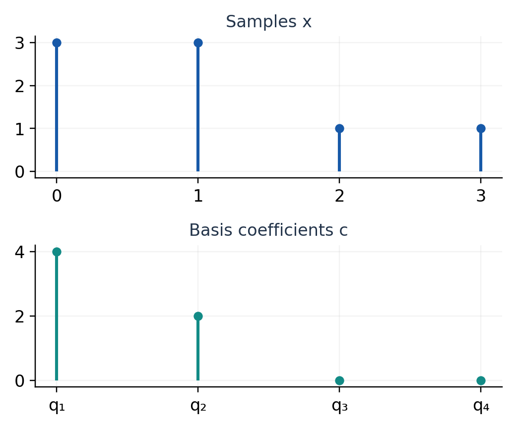
Worked Example 5.151 – Decode
The term 4q₁ gives (2,2,2,2); 2q₂ gives (1,1,−1,−1). Their sum is exactly (3,3,1,1).
The signal’s squared norm is 9+9+1+1=20, equal to the coefficient energy 4²+2²=20. This is the finite orthonormal energy identity.
Storage Detail
Sparse coefficients need their positions unless a fixed retained pattern is agreed in advance. Sending only “4 and 2” without identifying the basis and positions is not a complete standalone encoding.
Worked Example 5.152 – Keep Only the Average Direction
Retaining coefficient 4 alone reconstructs (2,2,2,2). The residual is (1,1,−1,−1), with squared norm 4. Retained energy is 16/20=80%.
Transform Is Not Compression
A full change of basis preserves the number of coefficients. A saving requires additional structure such as zeros, truncation, quantisation or statistical encoding.
Worked Example 5.153 – No Zero Coefficients
For x=(1,0,0,0), all four transform coefficients are 1/2. Keeping every coefficient reconstructs the sample exactly but stores as many coefficient values as input values.
Keeping only the first two yields (1/2,1/2,0,0), with squared error 1/2. Sparsity depends on both the signal and the chosen basis; a basis that compresses one pattern well may perform poorly for another.
45. Quantifying Approximation Loss
With an orthonormal basis, discarding coefficient cᵢ discards squared energy cᵢ². If x̂ retains a chosen subset, the squared reconstruction error is the sum of the squares of the omitted coefficients.
||x−x̂||²=Σ(i discarded) cᵢ²
For real data, this identity follows because the omitted basis directions are perpendicular. For complex coefficients, replace cᵢ² by |cᵢ|².
Worked Example 5.154 – One Discarded Direction
Using the four-sample basis, take x=(4,2,0,2). Its coefficients are (4,2,0,2). Keeping the first two yields x̂=(3,3,1,1), residual (1,−1,−1,1) and squared error 4.
The original squared energy is 24; retained energy is 20, giving 83.33% retained energy.

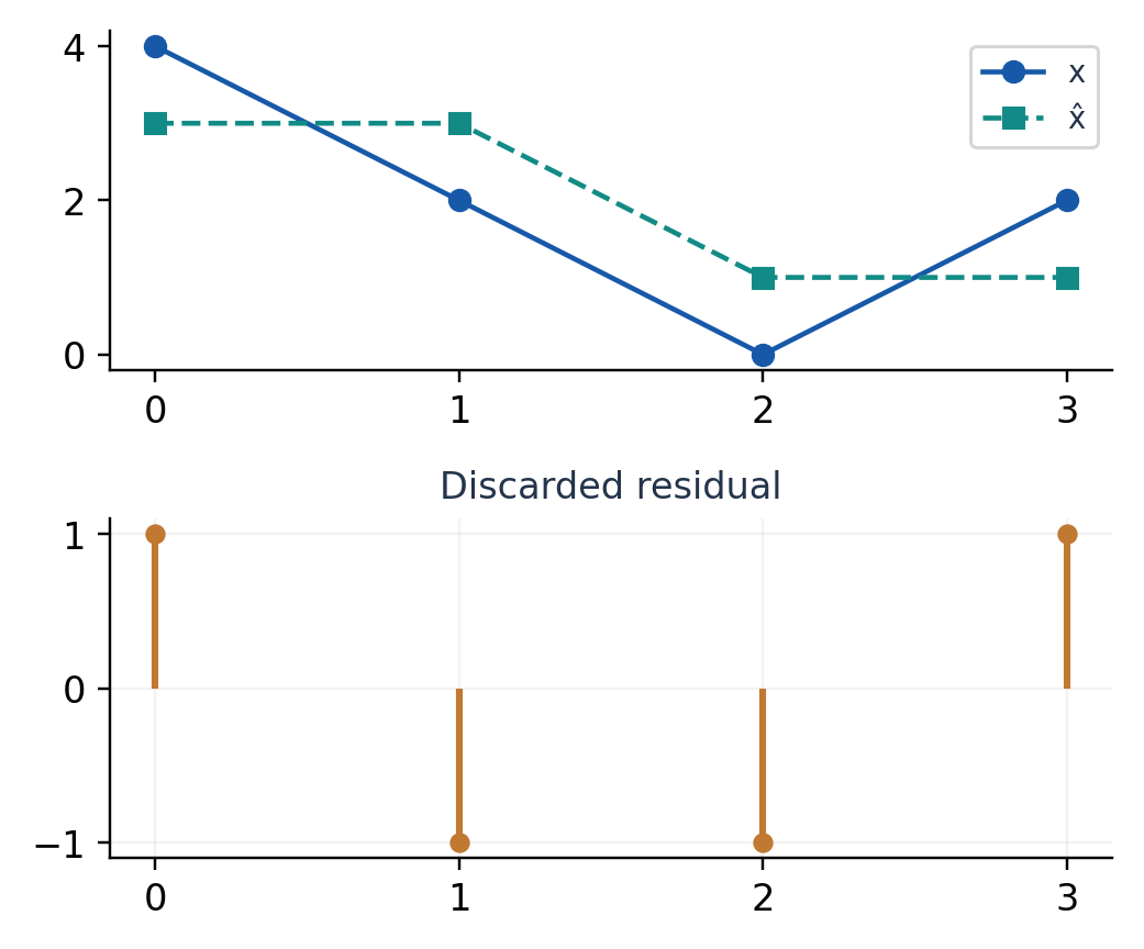
Worked Example 5.155 – Mean-Square Error
For four samples, MSE=||r||²/4=1 and RMSE=1 in the sample units. Relative Euclidean error is ||r||/||x||=2/√24=1/√6≈0.4082.
An 83.33% energy-retention figure therefore does not mean the relative vector error is 16.67%; energy is squared amplitude.
Choosing Retained Coefficients
For one fixed record in a complete orthonormal basis, keeping the r largest-magnitude coefficients minimises squared reconstruction error among all r-coefficient subsets.
A common fixed subspace for an entire dataset is a different optimisation problem. Its best directions depend on the dataset and centring assumptions.
Honest Reporting
State the basis, retained coefficients, error measure and sample count. Do not claim a universal visual or engineering quality from one energy percentage.
Small-amplitude discarded components may still contain safety-critical or diagnostically useful features.
Worked Example 5.156 – Equal-Magnitude Ties
For coefficients (4,2,0,2), a two-coefficient approximation may keep coefficients 1 and 2 or coefficients 1 and 4. Each retains energy 20 and discards energy 4 because the two smaller nonzero magnitudes tie.
The reconstructed sample patterns differ despite identical squared error. A single scalar quality score cannot reveal which structural feature was retained.

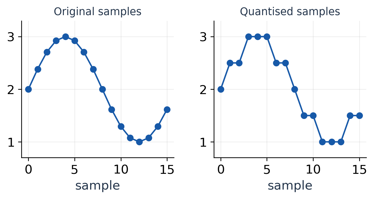
46. Signal Representation in a Basis
A sampled signal is a vector. A chosen basis separates it into known patterns: a constant component, slow changes, oscillations or local detail. The coefficients quantify how strongly each pattern is present.
Worked Example 5.157 – Mean and Difference
For two samples x=(5,1), use q₁=(1,1)/√2 and q₂=(1,−1)/√2. Coefficients are 3√2 and 2√2. Decoding gives (3,3)+(2,−2)=(5,1).
The first direction represents a shared level; the second represents contrast. The orthonormal coefficients include normalisation factors and are not literally the arithmetic mean and half-difference.

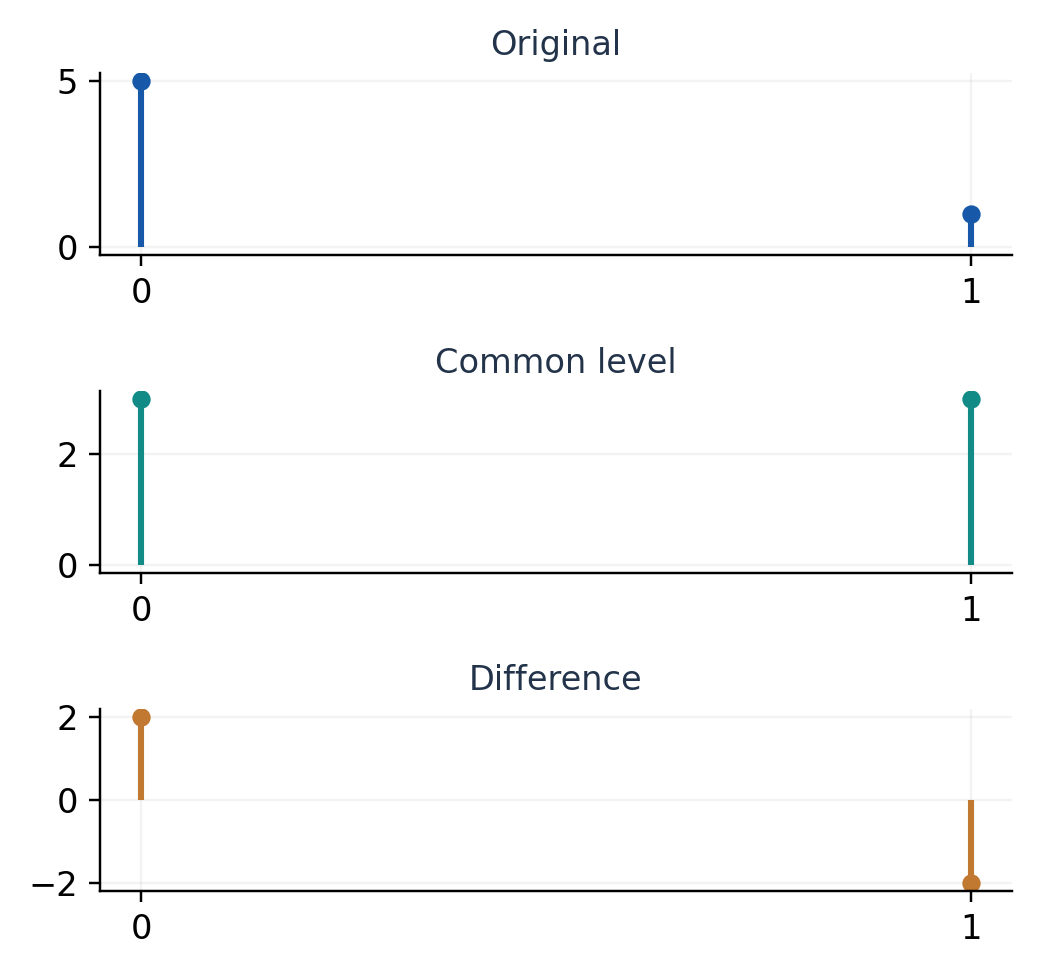
Worked Example 5.158 – Extract a Constant Component
For N samples, q₀=(1,…,1)/√N. Its coefficient is √N times the arithmetic mean. Its reconstructed contribution is the mean at every sample.
For x=(2,4,6,8), the mean is 5 and q₀=(1,1,1,1)/2. The coefficient is 10, giving constant contribution (5,5,5,5). The remaining vector is (−3,−1,1,3), whose entries sum to zero.
Superposition
A linear signal operation L satisfies:
L(ax+by)=aL(x)+bL(y)
Therefore knowing the operation on basis signals determines its result on every signal in their span.
Worked Example 5.159 – A Difference Operation
For D(x₁,x₂)=(x₂−x₁), D(5,1)=−4. Applying D to the constant contribution gives 0 and to (2,−2) gives −4, whose sum matches.
Model Boundary
Sampling rate, units and record length remain part of the signal description. Coefficients alone do not explain whether an oscillation is physically slow or fast.
Worked Example 5.160 – Zero-Mean Complement
For four samples, every vector perpendicular to the constant direction has entries summing to zero. The vectors (1,−1,0,0),(0,1,−1,0),(0,0,1,−1) form an independent basis of that three-dimensional zero-mean subspace.
Subtracting the sample mean therefore decomposes every record into a one-dimensional constant part and a three-dimensional zero-mean part, with no information loss if both are retained.

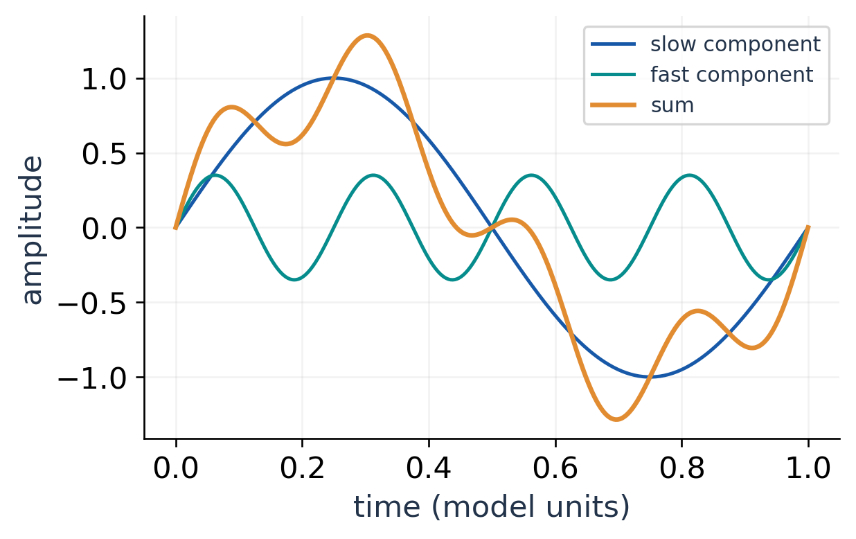
47. A Finite Frequency Representation
For four equally spaced samples, use real orthonormal patterns:
q₀=(1,1,1,1)/2
q_c=(1,0,−1,0)/√2
q_s=(0,1,0,−1)/√2
q_h=(1,−1,1,−1)/2
The patterns are constant, cosine-like, sine-like and alternating. They form a basis of R⁴, so every four-sample real record has a unique expansion.
Worked Example 5.161 – Oscillation Coefficients
For x=(3,1,−1,1), the coefficients in this order are (2,2√2,0,0). Thus the record is a constant level 1 plus (2,0,−2,0).
x=2q₀+2√2 q_c

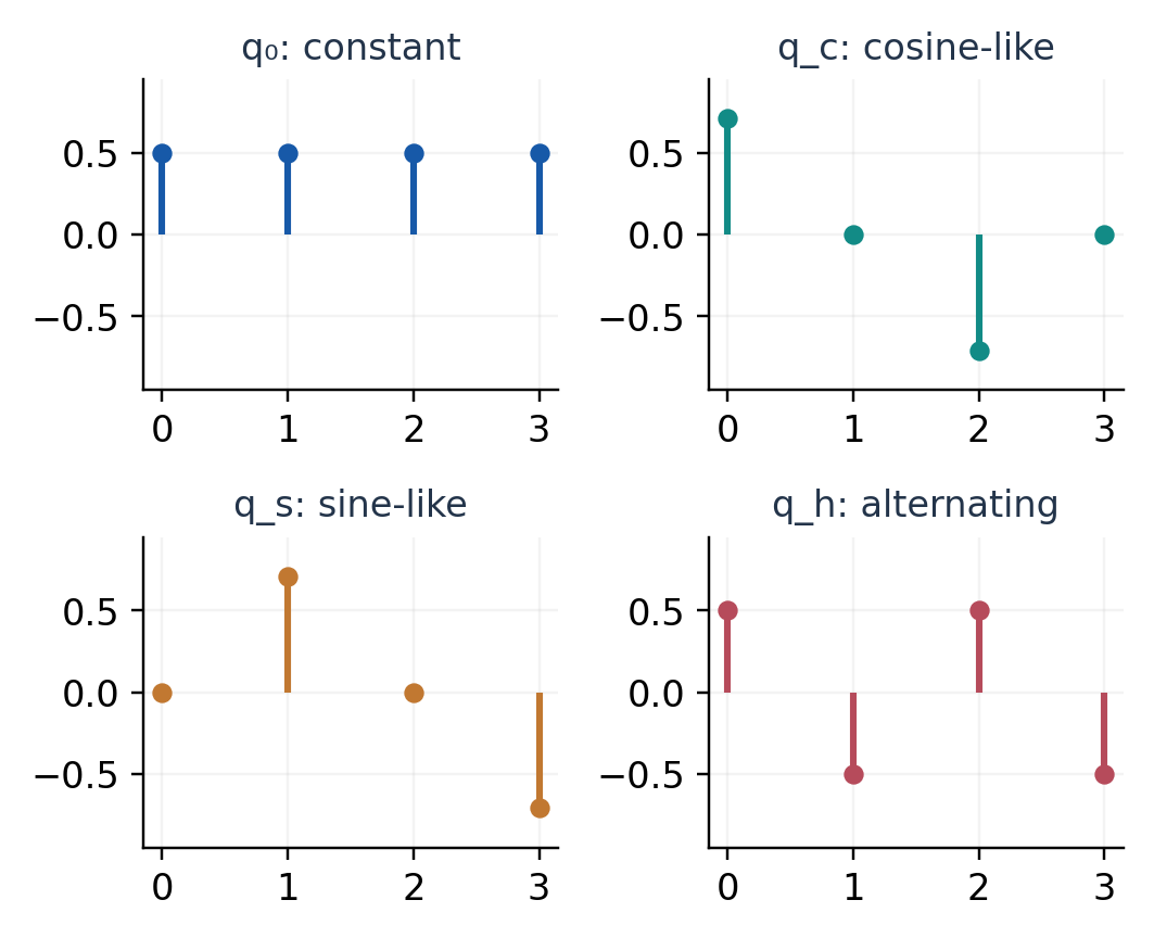
Worked Example 5.162 – Phase Matters
The record y=(1,3,1,−1) has coefficients (2,0,2√2,0). Its oscillation has the same amplitude as the preceding example but occupies the sine-like direction rather than the cosine-like direction.
Physical Frequency
If sample interval is Δt, these cosine-like and sine-like patterns complete one cycle over four sample intervals. Their discrete frequency corresponds to f=1/(4Δt). The alternating pattern corresponds to f=1/(2Δt).
This finite representation assumes a four-sample periodic pattern for frequency interpretation. It does not determine arbitrary behaviour between samples.
Complex Representation
A discrete Fourier transform uses complex exponential basis vectors. With consistent normalisation, it is another change of basis; retaining all coefficients permits exact discrete reconstruction.
No Invented Filtering Claim
Removing a high-frequency coefficient helps only when that direction is unwanted for the task. Fast genuine signal components can be damaged by the same operation.
The real four-sample example gives exact arithmetic without requiring a full Fourier-analysis course.

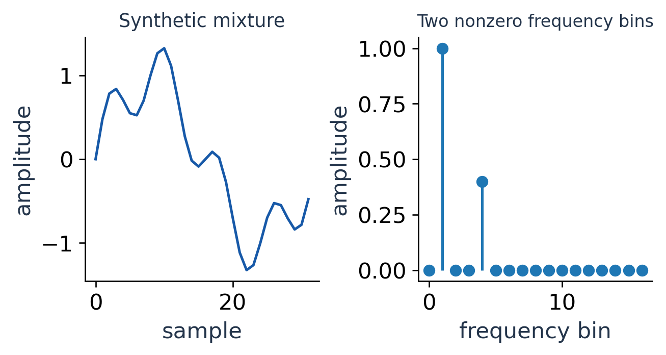
48. Noise Reduction by Projection
Assume the desired signal lies in a known subspace W. For measurement y=s+n with s in W, projection gives:
ŷ=P_W y=s+P_W n
Only the noise component perpendicular to W is removed.
y−ŷ=(I−P_W)n
Noise parallel to the signal subspace survives. If the true signal lies outside W, projection also removes part of the true signal.
Worked Example 5.163 – Pairwise Constant Model
Let W={(a,a,b,b)}. Its orthonormal basis is q₁=(1,1,0,0)/√2 and q₂=(0,0,1,1)/√2.
For y=(3.2,2.8,1.3,0.7), projection averages each pair, giving ŷ=(3,3,1,1). The removed residual is (0.2,−0.2,0.3,−0.3).

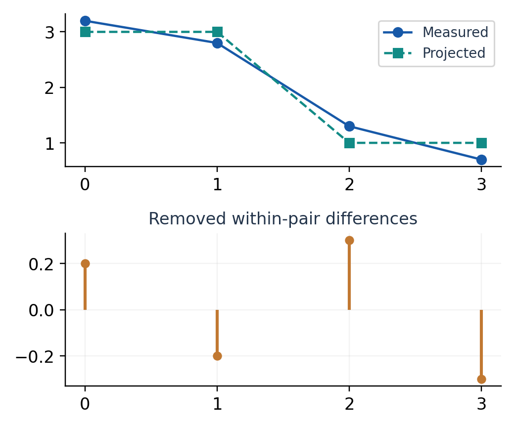
Worked Example 5.164 – Verify Orthogonality
The residual entries sum to zero within each pair, so rᵀq₁=rᵀq₂=0. Its squared norm is 0.04+0.04+0.09+0.09=0.26.
If the true signal is s=(3,3,1,1), this particular noise is entirely perpendicular to W and is removed exactly. That is a feature of the specified example, not a universal guarantee.
Worked Example 5.165 – Noise That Remains
For additional noise n=(0.1,0.1,−0.2,−0.2), n already lies in W. Projection preserves it completely, so averaging cannot separate it from a valid pairwise-constant signal.
Key Limitation
A denoiser distinguishes directions, not intentions. It cannot label a component “noise” merely because it is small or inconvenient. The assumed signal subspace must be justified.
Residual plots are useful diagnostics, but a small residual does not prove that the reconstructed signal is physically correct.
Worked Example 5.166 – Pairwise Projection Matrix
The averaging projection is block diagonal, with each 2×2 block equal to (1/2)[[1,1],[1,1]]. Its rank is 2 and its nullspace has basis (1,−1,0,0),(0,0,1,−1).
Those null directions are exactly the within-pair differences that are discarded. The retained subspace and discarded subspace are perpendicular and together account for all four sample directions.

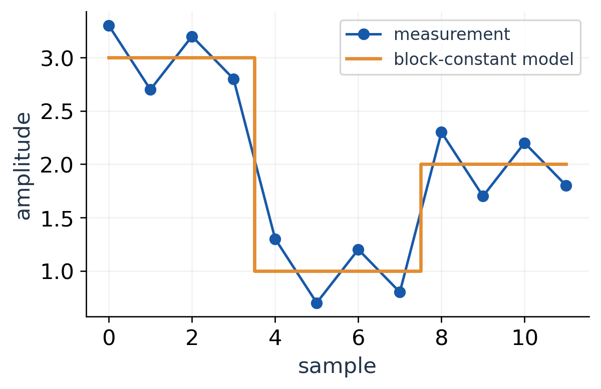
49. Trend Removal and Signal Bias
Suppose a record is expected to follow an affine trend in time. The sample vectors of all straight trends form span{1,t}. Projecting onto that subspace retains level and slope while discarding perpendicular fluctuations.
For three samples at t=0,1,2, take y=(1,2,2). The least-squares trend is (7/6,5/3,13/6), with residual (−1/6,1/3,−1/6).

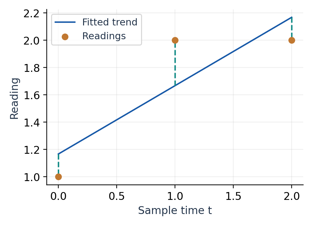
Worked Example 5.167 – A Perfectly Linear Record
For y=(2,3,4), the vector equals 2(1,1,1)+(0,1,2). It lies in the trend subspace, so projection leaves it unchanged and the residual is zero.
Worked Example 5.168 – A Real Peak Can Be Lost
The vector y=(0,1,0) has least-squares straight-trend fit (1/3,1/3,1/3), because its time-weighted residual also vanishes. A genuine middle peak is flattened by the model.
Thus a better-looking smooth output can still be a worse scientific representation. Model mismatch creates bias independently of random noise.
A Useful Decomposition
Write the true signal as the sum of an in-model component and a perpendicular component. Projection preserves the first and removes the second. Its reconstruction error therefore combines retained in-model noise with the negative of the removed true-signal component.
Validation Questions
- Does the chosen subspace represent plausible true signals?
- Which directions are removed and why?
- What physical units and scaling define the distance?
- Is reconstruction error acceptable for the intended decision?
Application Summary
Vector-space denoising is a model-based projection. Its benefit depends on the alignment of signal and noise with the retained directions, not simply on reducing the number of coefficients.
This completes the listed noise-reduction application while making its assumptions and limitations explicit.

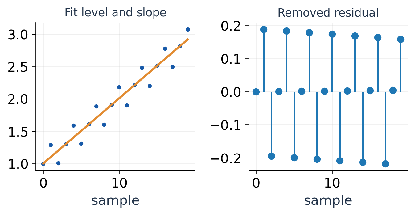

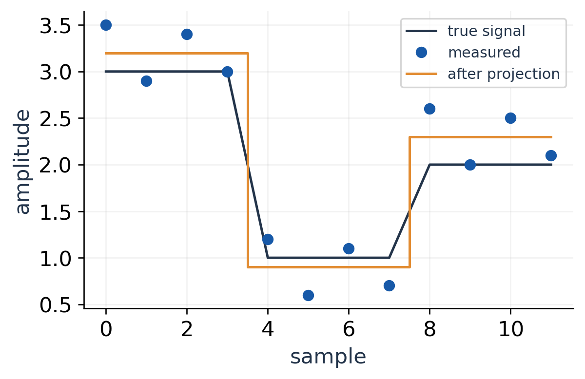
50. Binary Vector-Space Example
In F₂³, let u=(1,0,1), v=(0,1,1). The coefficients are binary, so their span contains just 0,u,v,u+v. These are 000,101,011,110.
Worked Example 5.169 – Independence over F₂
If au+bv=0, the first coordinate gives a=0 and the second gives b=0. Thus the pair is independent and forms a basis of its span. The span has dimension 2 and exactly 2²=4 elements.
W={(x₁,x₂,x₃):x₁+x₂+x₃=0 mod 2}

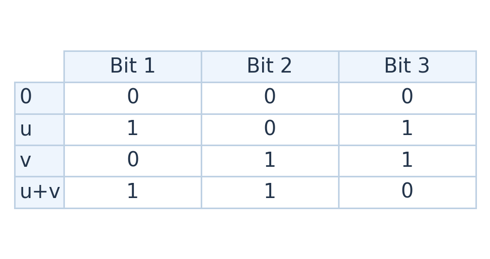
Worked Example 5.170 – Encode and Check
Message coefficients (1,1) encode as u+v=110. If the third bit flips, received word 111 has parity 1+1+1=1 modulo 2 and lies outside W, so an error is detected.
The parity result does not identify which bit changed. A single parity constraint is insufficient to correct arbitrary single-bit errors.
A Two-Error Limitation
Changing two bits preserves parity. For example, 000 can become 110, another valid codeword. This code cannot detect every double-bit change.
Field-Dependent Contrast
The same equation x₁+x₂+x₃=0 over R defines an infinite plane. Over F₂ it defines four binary vectors. Both have dimension 2 over their respective fields, but their element counts and geometry differ.
Core Concept Reinforced
A finite-dimensional vector space over F₂ has finitely many elements, while a positive-dimensional real space has infinitely many. Dimension counts basis size, not cardinality.
Binary coding is an additional compact illustration of fields and subspaces; the main syllabus applications remain data, signals and noise.
Worked Example 5.171 – Binary Coordinates Are Unique
The valid codeword 101 has coefficients (1,0), while 011 has coefficients (0,1) and 110 has coefficients (1,1). Independence guarantees that no second binary coefficient pair describes the same word.
Over R, the same generating vectors span z=x+y. The binary word 110 does not satisfy that real equation because 0≠1+1 in R. The codeword belongs only under the stated modulo-2 arithmetic.
51. Mixed Solved Problems
Worked Example 5.172 – Basis with Two Constraints
Let W={(x,y,z,w):x+y=0,z−w=0} in R⁴. Set y=s,w=t, giving x=−s,z=t.
(x,y,z,w)=s(−1,1,0,0)+t(0,0,1,1)
The two generators are independent by inspecting their second and fourth entries. They form a basis and dim W=2.
Worked Example 5.173 – A Polynomial Restriction
For p=a+bt+ct² with p(0)=p(1), the equation is b+c=0. Hence p=a+b(t−t²), with basis {1,t−t²}. The condition does not force p to be constant.
Worked Example 5.174 – A Matrix Intersection
A symmetric upper-triangular 2×2 matrix must have both off-diagonal entries zero. Thus the intersection is the diagonal subspace, with basis E₁₁,E₂₂ and dimension 2.
Worked Example 5.175 – Find a Dependence
For v₁=(1,2,1), v₂=(0,1,1), v₃=(2,5,3), observe v₃=2v₁+v₂. Hence 2v₁+v₂−v₃=0 is a nontrivial relation, and {v₁,v₂} is a basis of the span.
Worked Example 5.176 – A Small Compression Check
For x=(5,5,1,1) in the four-sample transform basis, coefficients are (6,4,0,0). Total energy is 36+16=52. Keeping only q₁ gives (3,3,3,3), residual (2,2,−2,−2) and squared error 16.
The retained-energy fraction is 36/52=9/13≈69.23%. Relative error is √(16/52)=2/√13, not 30.77%.
Worked Example 5.177 – One-Dimensional Projection
Project x=(2,0,1) onto span{u}, u=(1,1,1). The coefficient in u is (xᵀu)/(uᵀu)=3/3=1. Hence x̂=(1,1,1), residual (1,−1,0) and squared error 2.
Solution Habit
State the ambient space, operations and field; find the defining equations; identify free coefficients; and verify the final basis or reconstruction in the original problem.
Worked Example 5.178 – A Nonbasis Generating List
In P₂, the list 1,t,t²,1+t spans the space but is dependent because 1+t equals the sum of the first two vectors. Removing it leaves a basis of size 3.
Worked Example 5.179 – A Parameter Restriction
The two vectors (1,a,0),(0,1,a) are independent for every real a. The first coordinate of a zero combination forces the first coefficient zero, then the second coordinate forces the other zero. A parameter in a vector does not automatically create exceptional cases.
52. Short Proofs Worth Knowing
A Span Is a Subspace
Zero is obtained by choosing every coefficient zero. If u=Σaᵢvᵢ and w=Σbᵢvᵢ, then αu+βw=Σ(αaᵢ+βbᵢ)vᵢ, another combination of the generators. Therefore their span is closed under all linear combinations.
A Basis Gives Unique Coordinates
Spanning gives existence. If Σaᵢvᵢ=Σbᵢvᵢ, subtract the equations. Independence of the basis forces aᵢ−bᵢ=0 for each i, proving uniqueness.
Removing Redundancy Preserves Span
If vₖ is already a combination of the other generators, replace every coefficient times vₖ by that combination. Every old vector is still generated by the remaining list; the reverse containment is immediate.
These proofs explain why a basis is an efficient exact description rather than merely a convenient list of vectors.
Nonzero Orthogonal Vectors Are Independent
Assume Σaᵢuᵢ=0 for mutually orthogonal nonzero vectors. Take the inner product with uⱼ. All cross terms vanish, giving aⱼ||uⱼ||²=0. Since ||uⱼ||²>0, aⱼ=0 for every j.
Projection Is Closest
Let x=x̂+r, with x̂ in W and r perpendicular to W. For any w in W, x−w=r+(x̂−w). Orthogonality gives:
||x−w||²=||r||²+||x̂−w||²
The unique minimum is at w=x̂.
Intersection Is a Subspace
For u,v in U∩W, both vectors lie in each subspace. Every combination au+bv remains in U and remains in W, hence lies in their intersection. Zero belongs to both.
Proof Quality
Use arbitrary elements and state the reason each operation is valid. Numerical demonstrations illustrate a theorem but do not replace its general argument.
For dimension claims, an explicit basis with a spanning and independence argument is often more convincing than a bare count of symbols.
Zero-Space Containment Proof
Every subspace contains the ambient zero vector: take any member u, which exists because the subspace is nonempty, and use scalar closure to obtain 0u=0. Thus a nonempty subset excluding zero cannot be a subspace.
Basis Removal Contradiction
Removing a vector from an independent basis destroys spanning. Otherwise the removed vector would be a combination of those remaining, creating a nontrivial zero relation in the original basis. A basis therefore has no removable member if its span is to stay unchanged.
53. Common Mistakes and Repairs
Zero Test Treated as Sufficient
A unit disc contains zero but fails scalar closure: (1,0) is inside, while 2(1,0) is outside. Check addition and every allowed scalar as well.
Only Pairs Tested
The list e₁,e₂,e₁+e₂ is dependent although each pair is independent. Solve the full zero-combination problem for the entire list.
Ambient Length Called Dimension
Vectors in the plane x+y+z=0 have three entries but only two free parameters. Its dimension is 2. A basis proves the count.
Reduced Columns Used as a Column Basis
Use pivot positions from elimination, then select the corresponding original columns. Reduced nonzero rows are appropriate for row space instead.
Polynomial Degree Exactly n Used
Include degree at most n and the zero polynomial. Degree exactly n is not closed under zero scaling or cancellation.
Arbitrary B Used in BBᵀ
The formula x̂=BBᵀx requires orthonormal columns. With a nonorthonormal independent basis, solve BᵀBc=Bᵀx instead.
A Full Transform Called Compression
Retaining every coefficient is an exact coordinate change. Explain what is omitted, quantised or encoded and include basis overhead in storage counts.
Every Residual Called Noise
A residual can include genuine signal outside the assumed model. State the signal-subspace assumption and examine model mismatch.
Scalar Field Omitted
The pair {1,i} is independent over R but dependent over C. A dimension statement must use the field for which its basis is valid.
Error Energy Confused with Error Norm
If retained energy is 84%, relative Euclidean error is √0.16=40%, not 16%, assuming orthogonal decomposition and the same normalisation.
Final Correction Rule
Return to the exact definition being tested: field, closure, span, independence, basis, dimension or approximation metric. Many errors come from using a shortcut whose assumptions are absent.
A Final Worked Diagnostic
Consider W={(x,y):x+y=1}. It fails the zero test, so stop: it is not a subspace. Its direction space x+y=0 has basis (1,−1), but that basis does not span W under ordinary linear combinations.
The correct affine description is:
W=(1,0)+span{(1,−1)}
This one example separates membership, a direction basis, an offset and subspace status in a form useful for modelling data.
54. Short-Answer Checks
What Is a Field?
A set with addition and multiplication obeying the field laws, including a distinct multiplicative identity and inverses for every nonzero element. R, C and F₂ are examples; Z is not a field under usual operations.
What Is a Vector Space?
A nonempty collection with vector addition and scalar multiplication over a field satisfying closure and the vector-space laws. The elements need not be geometric arrows.
What Makes a Subset a Subspace?
It contains zero and is closed under addition and every scalar from the same field, using the ambient operations. Homogeneous linear restrictions provide common examples.
What Is Linear Dependence?
There is a zero combination with at least one nonzero coefficient. Equivalently, one listed vector is a combination of the others.
What Is Independence?
The only zero combination is the one with every coefficient zero. It gives uniqueness of representation within the span.
What Is a Basis?
An independent spanning set. Every vector has a unique finite combination of its basis vectors. Basis order determines coordinate order.
What Is Dimension?
The size of a basis over the stated field. All bases of a finite-dimensional space have the same size. The zero space has dimension 0.
Does a Basis Have to Be Orthogonal?
No. Orthogonality is an additional geometric property available after choosing an inner product. It simplifies coefficient calculations but is not required for a basis.
How Do Subspaces Help Compression?
Records represented by r independent directions can be stored as r coefficients, together with a shared model and any offsets. Approximate compression may discard directions and introduces reconstruction error.
How Does Projection Reduce Noise?
It removes components perpendicular to the assumed signal subspace. Noise inside that subspace remains, and true signal outside it is also removed.
Answer Standard
Give the definition first, then one short example or qualification. Keep field, operations and model assumptions visible whenever they change the conclusion.
Can the Same Vector Have Different Coordinates?
Yes, in different ordered bases. In one fixed basis its coordinates are unique. If a generating list is dependent, even one fixed list can give multiple coefficient descriptions, which is exactly why it is not a basis.
Does Zero Residual Prove a Model Is True?
No. It proves the observed vector lies in the chosen model subspace under the stated arithmetic. It does not establish that the model explains unobserved measurements or the physical mechanism.
55. Formula and Method Sheet
Vector-Space Identities
0v=0
a0=0
(−1)v=−v
Subspace Test
A nonempty subset is a subspace if au+bv remains in it for every pair of members and all allowed scalars.
Dependence and Rank
Ac=0 has only c=0 ⇔ independent columns ⇔ ker A={0}
rank A=k for k independent columns
Basis and Coordinates
x=S_B[x]_B
[x]_C=S_C⁻¹S_B[x]_B
The inverse formula assumes square basis matrices for the same full coordinate space. A proper-subspace basis may give a rectangular matrix.
Dimension Counts
dim Pₙ=n+1
dim M_(m×n)=mn
rank A+nullity A=n
Here n is the number of columns of A.
Sum and Intersection
dim(U+W)=dim U+dim W−dim(U∩W)
The sum is direct when U∩W={0}; then each decomposition is unique.
Orthogonal Applications
For real orthonormal columns Q:
c=Qᵀx
x̂=Qc
r=x−x̂
Qᵀr=0
||x||²=||x̂||²+||r||²
For an independent real basis B:
BᵀBc=Bᵀx
x̂=Bc
Compression Error
||r||²=Σ(i discarded) |cᵢ|²
This coefficient formula assumes orthonormal directions.
For N samples:
MSE=||r||²/N
RMSE=||r||/√N
Final Checks
State the field; verify zero and closure; distinguish spanning from independence; prove the basis; count free directions; reconstruct coefficients; and report what the model discards.
Fast Method Selection
For a homogeneous restriction, solve for free parameters to construct a basis. For a listed set, put vectors in columns and find pivots. For polynomial identities, compare coefficients. For a best Euclidean reconstruction, use orthogonal projection with its assumptions checked.
After a basis change, decode once to verify the original vector. After truncation, report the residual norm and distinguish it from squared error. For binary vectors, reduce every coefficient calculation modulo 2.


