


University: Dr. A.P.J. Abdul Kalam Technical University (AKTU)
Programme: B.Tech First Year, Semester I
Course Code: AAS103D
Stream: CSE
Unit: II – Multiple Integrals
Equation notation: ∫[a,b] means integration from lower limit a to upper limit b. In nested integrals, evaluate the rightmost differential first. Powers written as x^(m−1) mean x raised to (m−1).
Unit II Introduction
A multiple integral adds contributions spread across an area or a volume. The contribution may represent height, mass density, image intensity or probability density. The region and the small area or volume element are as important as the integrand.
This unit builds double and triple integrals from geometric slices, then develops coordinate changes, Beta and Gamma functions and Dirichlet’s integral. Applications connect the mathematics to image processing, data density estimation and probability models.
Complete Syllabus Map
| Topic | PDF Pages |
|---|---|
| Double integrals and planar regions | 2–6 |
| Change of order of integration | 7–10 |
| Polar coordinates, area and volume | 11–16 |
| General change of variables | 17–19 |
| Triple integrals and solids | 20–26 |
| Gamma function and properties | 27–31 |
| Beta function and properties | 32–36 |
| Dirichlet’s integral | 37–40 |
| Image, density and AI applications | 41–48 |
| Solved revision and formula sheets | 49–54 |
Central Idea
Sketch the region, choose a useful order or coordinate system, write every bound, include the correct measure, then integrate and check the result.
Reading an Integral Correctly
For dy dx, integrate with respect to y first. Hold x fixed while using the inner limits. After that step, the remaining expression must depend only on x.
For dz dy dx, integrate with respect to z first, then y, then x. A bound for an inner variable may depend on variables that remain outside it; an outermost bound cannot depend on an already integrated variable.
Notation and Assumptions
| Symbol | Meaning |
|---|---|
| D | Region in the xy-plane |
| E | Solid region in space |
| dA, dV | Area and volume elements |
| J | Jacobian determinant |
| Γ(s) | Gamma function |
| B(p,q) | Beta function |
| f(x,y) | Integrand or a stated joint density |
| ρ(x,y) | Mass or count density |
Unless a problem states otherwise, coordinates and parameters are real. Formula conditions such as p>0 are part of the result. Application models are explicitly specified mathematical examples, not measured performance claims.
Working Habits
- Draw and label boundary intersections before reversing limits.
- Distinguish geometric volume from signed integration.
- Use an absolute Jacobian for area or volume.
- Check convergence before applying improper-integral identities.
- A probability density must be nonnegative and integrate to one.
1. What a Double Integral Adds
Partition a bounded region D into small cells. Choose a point in each cell and multiply the function value there by that cell’s area. Add these products and refine the partition.
∬_D f(x,y) dA = lim Σᵢ f(xᵢ,yᵢ) ΔAᵢ.
For a continuous function on a closed bounded region with a well-behaved boundary, this limit gives the double integral. Each term is a contribution, not just a function value.


Geometric Meaning
If f≥0, the integral is the volume between z=f and the plane z=0 over D. If f changes sign, contributions below the plane subtract. Geometric volume instead integrates the nonnegative height difference between the upper and lower surfaces.
Units and a First Calculation
If f has units of metres and dA has units of square metres, the integral has units of cubic metres. If f is mass per square metre, the same operation gives mass.
Worked Example 2.1 – Constant Height
A plate-shaped base occupies 0≤x≤3 and 0≤y≤2. Above it is a constant height of 4. The base area is 6, so:
∬_D 4 dA = 4(3)(2) = 24.
The result agrees with the familiar rectangular-prism formula. This is a useful check on bounds and units.
Worked Example 2.2 – A Coarse Sum
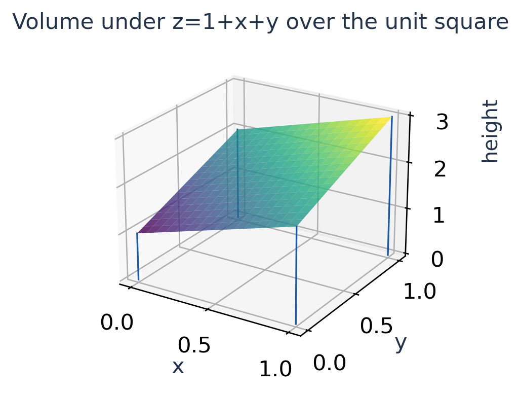
Divide the unit square into four equal cells, each of area 1/4. For f=1+x+y, use cell centres (1/4,1/4), (3/4,1/4), (1/4,3/4), (3/4,3/4).
The heights are 3/2, 2, 2 and 5/2. Thus:
S = (1/4)(3/2 + 2 + 2 + 5/2) = 2.
Here the midpoint sum equals the exact integral because the function is affine on a rectangle. General curved surfaces need not be integrated exactly by such a coarse sum.
Remember
The cell area is essential. Adding only the four heights would give 8, which has the wrong scale and does not approximate the integral.

2. Double Integrals on Rectangles
Let D=[a,b]×[c,d]. For a continuous integrand, Fubini’s theorem allows evaluation as either of two iterated integrals:
∬_D f dA = ∫[a,b] ∫[c,d] f dy dx = ∫[c,d] ∫[a,b] f dx dy.
The inner antiderivative treats the outer variable as a constant. Insert the inner limits before beginning the outer integration.
Worked Example 2.3 – Polynomial on a Rectangle
Evaluate f=x+2y on 0≤x≤2, 0≤y≤1.
I = ∫[0,2] [xy+y²] evaluated from y=0 to y=1 dx.
I = ∫[0,2] (x+1) dx = 4.
The region has area 2. Since the average value of x+2y is 2 on this rectangle, a total of 4 is reasonable.


Reversing a Rectangular Order
The same example can be checked with x first:
I = ∫[0,1] [x²/2+2xy] evaluated from x=0 to x=2 dy.
I = ∫[0,1] (2+4y) dy = 4.
Changing order changes the intermediate expression, not the region or the final value.
Worked Example 2.4 – Product Integrand
On the unit square, evaluate x²y.
I = (∫[0,1] x² dx)(∫[0,1] y dy).
I = (1/3)(1/2) = 1/6.
This separation works because both the function and the rectangular domain separate into independent x and y factors. A triangular domain does not usually permit the same shortcut.
When Exchanging Order Needs Care
Continuity on a bounded rectangle is a convenient sufficient condition. For improper integrals, absolute integrability justifies exchanging order; nonnegative measurable integrands also allow order exchange with a possibly infinite value.
One should not infer convergence from a formal antiderivative alone. A singularity or infinite boundary needs a separate limit check.
Method
Copy the outer differential beside its limits. In dy dx, y is inner and x is outer. This simple notation check prevents most first-step mistakes.
3. Useful Integral Properties
Linearity allows sums and constants to be handled separately:
∬_D (af+bg) dA = a∬_D f dA + b∬_D g dA.
If D is divided into nonoverlapping pieces, add the integrals over those pieces. Shared boundary curves have zero area in the ordinary examples considered here.
If m≤f≤M on a region of area A, then:
mA ≤ ∬_D f dA ≤ MA.
These bounds provide a quick independent check on a numerical answer.
Worked Example 2.5 – A Magnitude Check
For f=x+y on the unit square, 0≤f≤2 and A=1. The exact integral is 1, which lies between 0 and 2.
A claimed answer of 5 would be impossible even before reworking the antiderivative.
Symmetry Saves Calculation
If a region is symmetric under x→−x and f changes sign under that reflection, contributions cancel in pairs. The double integral is zero, provided the integral exists.
Worked Example 2.6 – Odd Integrand
Let D be the disk x²+y²≤4. The function x(x²+y²) is odd in x. Hence:
∬_D x(x²+y²) dA = 0.
No polar calculation is needed. The cancellation follows from matching each point (x,y) with (−x,y).


Limits of the Shortcut
Symmetry of the integrand alone is insufficient. On a right half-disk, x does not have a negative-x partner inside the region.
Similarly, a nonnegative nonzero function over a region of positive area has a positive integral; cancellation cannot make it zero.
Check Before Integrating
Look for reflection symmetry, constant factors and separable products. Use them only after checking that the domain preserves the required symmetry or independence.
4. Nonrectangular Regions
A vertically simple region has a fixed x-range and lower and upper y-boundaries:
D: a≤x≤b, g₁(x)≤y≤g₂(x).
∬_D f dA = ∫[a,b] ∫[g₁(x),g₂(x)] f dy dx.
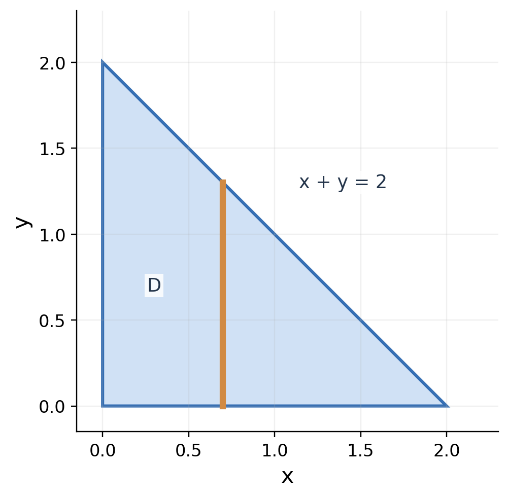
Draw a vertical line through the interior. Its entry and exit points determine the inner limits. The projection of the whole region on the x-axis determines the outer limits.

Worked Example 2.7 – Area of a Triangle
Set the integrand equal to one:
A = ∫[0,2] ∫[0,2−x] 1 dy dx.
A = ∫[0,2] (2−x) dx = 2.
The result matches one-half base times height.
Worked Example 2.8 – Integrate x+y
Use the same triangle. With x fixed, y runs from 0 to 2−x.
I = ∫[0,2] [xy+y²/2] evaluated from y=0 to y=2−x dx.
Simplify the inner result before integrating again:
x(2−x)+(2−x)²/2 = 2−x²/2.
I = [2x−x³/6] evaluated from x=0 to x=2 = 8/3.
An independent check uses the centroid. The average x and y over this uniform triangle are both 2/3, so the average of x+y is 4/3. Multiply by area 2 to recover 8/3.
Worked Example 2.9 – Integrate xy
I = ∫[0,2] ∫[0,2−x] xy dy dx.
I = (1/2)∫[0,2] x(2−x)² dx = 2/3.
The product shortcut from a rectangle would be wrong here: the permitted y-range shrinks as x increases.
Boundary Check
At x=0 the slice has height 2; at x=2 it shrinks to zero. A proposed pair of limits should reproduce both endpoint behaviours.
5. Regions Between Curves
For a region between y=g(x) and y=h(x), first find their intersections. Then test an interior x-value to identify which curve is higher.
Worked Example 2.10 – Parabola and Line
The curves y=x² and y=x intersect when x²=x, so x=0 or 1. Between them, x≥x². Therefore:
D: 0≤x≤1, x²≤y≤x.


Area
A = ∫[0,1] (x−x²) dx = 1/6.
Use upper minus lower, not the sum of the curves. The width of a slice must be nonnegative throughout the interval.
Worked Example 2.11 – Integrate x over D
I = ∫[0,1] ∫[x²,x] x dy dx.
I = ∫[0,1] (x²−x³) dx = 1/12.
Because x ranges from 0 to 1, the answer must lie between 0 and A=1/6. The value 1/12 passes this check.
Worked Example 2.12 – Integrate y over D
I = (1/2)∫[0,1] (x²−x⁴) dx = 1/15.
The two integrals need not be equal: the region is not symmetric under interchanging x and y.
Horizontal Description
Solve the boundaries for x. Since y=x gives x=y and y=x² gives x=√y in the first quadrant:
0≤y≤1, y≤x≤√y.
At y=1/4, the horizontal slice runs from x=1/4 to x=1/2. This interior test verifies the direction of the inequalities.
Sketching Trick
Mark all intersections and one interior slice before writing an integral. A small accurate sketch is more useful than a decorative large drawing with unlabelled axes.
6. Change of Integration Order
Changing order means describing the same set of points with a new family of slices. Merely exchanging dx and dy while leaving the limits unchanged almost always changes the problem.
A Reliable Procedure
- Step 1: Translate the old limits into inequalities.
- Step 2: Sketch every boundary and mark intersections.
- Step 3: Project the region onto the new outer axis.
- Step 4: Read entry and exit curves along the new inner direction.
- Step 5: Split the region if one boundary formula cannot cover all slices.


Worked Example 2.13 – A Unit Triangle
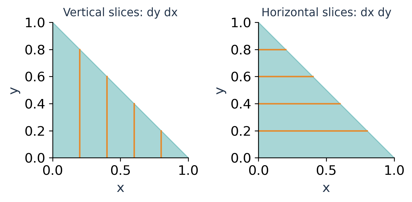
∫[0,1] ∫[0,1−x] f(x,y) dy dx = ∫[0,1] ∫[0,1−y] f(x,y) dx dy.
The line x+y=1 is solved for the inner variable in each description.
Check the New Limits
For this triangle, both descriptions include (1/4,1/4) and exclude (3/4,3/4). They also have the same vertices (0,0), (1,0), (0,1).
Worked Example 2.14 – Verify by Integration
Choose f=x+2y. In the original order:
I = ∫[0,1] [x(1−x)+(1−x)²] dx.
I = ∫[0,1] (1−x) dx = 1/2.
In the reversed order:
I = ∫[0,1] [x²/2+2yx] evaluated from x=0 to x=1−y dy.
The integrand becomes (1−y)²/2+2y(1−y). Its integral is also 1/2.
Why Order Matters Computationally
The region determines which orders are valid; the integrand helps decide which valid order is easier. An awkward antiderivative in one direction may become a one-step substitution after reversing the order.
Warning
The equation for the boundary is unchanged, but its role changes. In the new order, solve it for the new inner variable and use the new outer range.

7. Reversing a Sloping Strip
Worked Example 2.15 – Reverse and Evaluate
Consider:
I = ∫[0,2] ∫[x/2,1] (x+y) dy dx.
The inequalities are 0≤x≤2 and x/2≤y≤1. Equivalently, 0≤y≤1 and 0≤x≤2y.
I = ∫[0,1] ∫[0,2y] (x+y) dx dy.
I = ∫[0,1] (2y²+2y²) dy = 4/3.

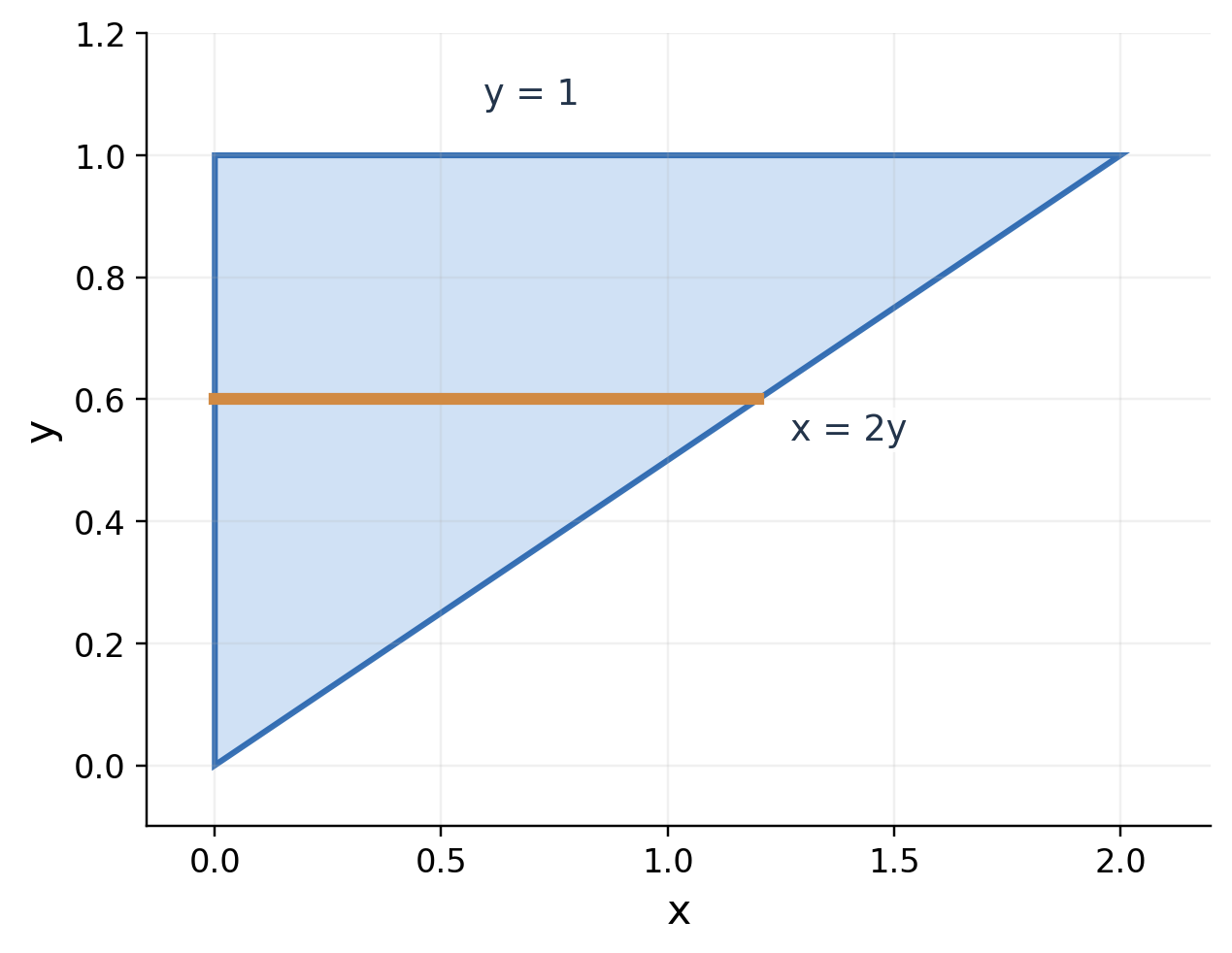
A common wrong upper x-limit is y/2. Solving y=x/2 actually gives x=2y. Check the boundary point (2,1).
Worked Example 2.16 – Reverse a Parabolic Region
I = ∫[0,1] ∫[x²,1] y dy dx.
The region is above y=x², below y=1 and to the right of x=0. For fixed y, x runs from 0 to √y:
I = ∫[0,1] ∫[0,√y] y dx dy.
I = ∫[0,1] y^(3/2) dy = 2/5.
In the original order, the inner integral gives (1−x⁴)/2, whose integral is also 2/5.
Distinguish Two Similar Regions
The region y between x² and 1 differs from the region y between x² and x. The former has the horizontal top y=1; the latter has the sloping top y=x.
Replacing one by the other changes both the area and the integral. Always preserve every original inequality.
Quick Test
At y=1/4, the first region permits 0≤x≤1/2. The region between the parabola and line instead permits 1/4≤x≤1/2.
8. When a Reversed Region Splits
A single set of old limits can require two integrals in the new order. This happens when the new entry or exit boundary changes at an intersection or corner.
Worked Example 2.17 – A Triangular Cap
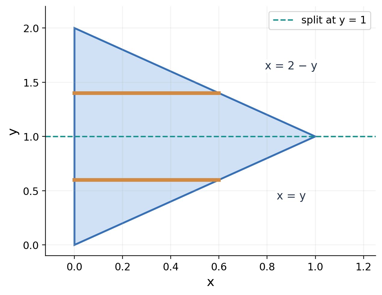
Take 0≤x≤1 and x≤y≤2−x. The vertices are (0,0), (0,2) and (1,1).
For 0≤y≤1, the right boundary is x=y. For 1≤y≤2, it is x=2−y.
∫[0,1] ∫[x,2−x] f dy dx
= ∫[0,1] ∫[0,y] f dx dy + ∫[1,2] ∫[0,2−y] f dx dy.

Worked Example 2.18 – Area and First Moment
With f=1, the two areas are:
A = ∫[0,1] y dy + ∫[1,2] (2−y) dy = 1.
With f=y, the same split gives:
I = ∫[0,1] y² dy + ∫[1,2] y(2−y) dy.
I = 1/3 + 2/3 = 1.
This agrees with the triangle’s centroid y-coordinate, which is 1. Its area is 1, so the first y-moment is also 1.
Why One Shortcut Fails
Using 0≤x≤y for the entire interval 0≤y≤2 would include points outside the triangle when y>1. Using 0≤x≤2−y everywhere would include extra points when y<1.
How to Locate the Split
Find where competing boundaries meet: y=2−y gives y=1. Draw one horizontal slice below and another above this level. The smaller permitted right endpoint determines the valid bound.
Exam Presentation
Write both pieces with the same integrand and differential order. A labelled split level makes the reasoning visible even before the arithmetic.
9. Order Change Can Unlock an Integral
An elementary-looking double integral may contain an inner antiderivative that is not elementary. The double integral itself can still have a simple exact value after reversing order.
Worked Example 2.19 – Exponential of y²
Evaluate:
I = ∫[0,1] ∫[x,1] e^(y²) dy dx.
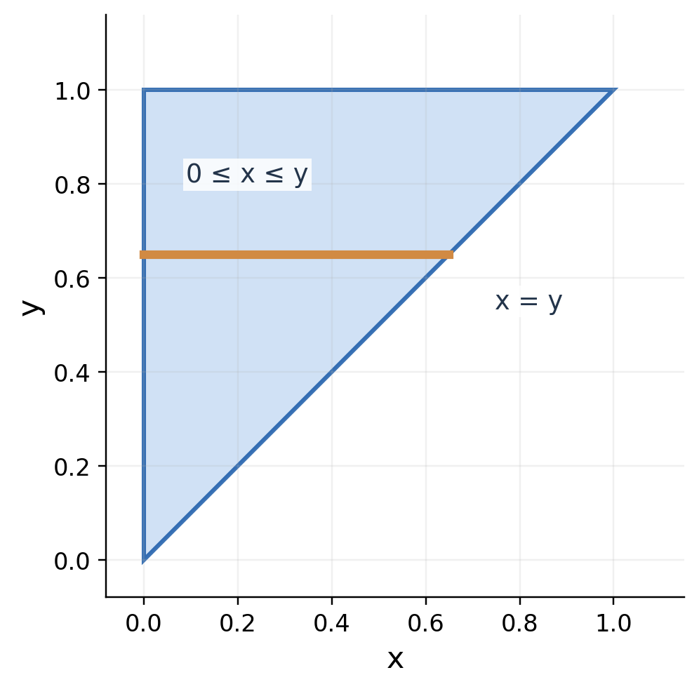
The region is 0≤x≤y≤1. Reverse the order:
I = ∫[0,1] ∫[0,y] e^(y²) dx dy.
I = ∫[0,1] y e^(y²) dy = (e−1)/2.
The x-integration supplies the factor y needed for the substitution u=y².

Worked Example 2.20 – Cosine of x²
I = ∫[0,1] ∫[y,1] cos(x²) dx dy.
Here 0≤y≤x≤1. In the other order:
I = ∫[0,1] ∫[0,x] cos(x²) dy dx.
I = ∫[0,1] x cos(x²) dx = (sin 1)/2.
Angles are in radians. The region has area 1/2 and cos(x²) lies between cos 1 and 1, so the answer must lie between (cos 1)/2 and 1/2. The exact result satisfies that bound.
What the Method Does Not Claim
This does not give an elementary antiderivative for e^(y²) or cos(x²). It changes the integration sequence over a two-dimensional region and introduces a useful factor through the other variable.
Choosing an Order
- If the integrand depends only on y, try x first.
- If it depends only on x, try y first.
- If both choices are easy, prefer simpler region bounds.
Remember
Change the geometry and the order together. An easier antiderivative is useful only when the reversed limits describe exactly the original region.
10. Polar Coordinates and Area
For circles, disks and rotationally symmetric functions, use:
x = r cos θ, y = r sin θ.
dA = r dr dθ, r≥0.
A small polar cell has radial thickness dr and approximate arc length r dθ. Their product explains the extra factor r.


Change-of-Variables Formula
∬_D f(x,y) dA = ∬_S f(r cos θ,r sin θ) r dr dθ.
The function, domain and area element all change. Substituting only x²+y²=r² is incomplete.
Finding Polar Bounds
A disk of radius a centred at the origin has 0≤r≤a and 0≤θ≤2π. A first-quadrant quarter-disk uses 0≤θ≤π/2 instead.
Worked Example 2.21 – Disk Area
A = ∫[0,2π] ∫[0,a] r dr dθ.
A = 2π(a²/2) = πa².
Without the Jacobian factor, the wrong answer would be 2πa, which has units of length rather than area.
Worked Example 2.22 – A Radial Quadratic
For x²+y²≤a²:
∬_D (x²+y²) dA = ∫[0,2π] ∫[0,a] r³ dr dθ = πa⁴/2.
The original integrand contributes r² and the area element contributes another r.
Bound Checks
Every ray in the chosen angular interval should enter and leave the region at the written radial limits. Negative radius is unnecessary for these standard regions and can create duplicate coverage.
Polar Checklist
Transform x and y, transform the boundary, include r, identify the full angular interval, and count the region only once.


11. Annuli, Sectors and Symmetry
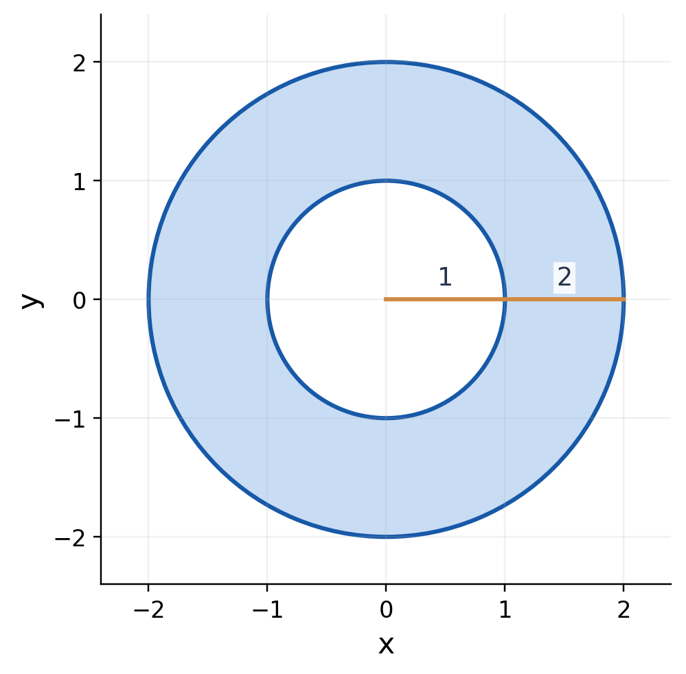
An annulus a≤r≤b removes the central disk. A sector also restricts θ to an interval [α,β].
Worked Example 2.23 – Weighted Annulus
Evaluate x²+y² over 1≤x²+y²≤4.
I = ∫[0,2π] ∫[1,2] r³ dr dθ.
I = (2π/4)(16−1) = 15π/2.
The area is 3π, and the integrand ranges from 1 to 4. Thus 3π≤I≤12π, consistent with 15π/2.

Worked Example 2.24 – A Quarter-Disk Moment
Evaluate x over the first-quadrant unit disk.
I = ∫[0,π/2] ∫[0,1] r² cos θ dr dθ.
I = (1/3)[sin θ] evaluated from θ=0 to θ=π/2 = 1/3.
The integrand is x=r cos θ, not simply r. Discarding cos θ changes the function.
Worked Example 2.25 – Second Moment of a Disk
For a disk of radius a:
∬_D x² dA = (∫[0,a] r³ dr)(∫[0,2π] cos²θ dθ).
I = πa⁴/4.
By symmetry the y² integral is identical. Adding them gives πa⁴/2, agreeing with the radial calculation.
A Sector-Area Formula
With 0≤r≤a and α≤θ≤β:
A = (a²/2)(β−α).
The angular difference must be measured in radians. A full turn gives β−α=2π and recovers the disk formula.
12. A Circle Away from the Origin
Polar coordinates can also simplify circles passing through the origin. Rewrite the Cartesian boundary before choosing the angular interval.
Worked Example 2.26 – Shifted Disk Area
Consider x²+y²≤2ax, where a>0. This is a circle centred at (a,0) with radius a.
Substitution gives r²≤2ar cos θ. With r≥0:
−π/2≤θ≤π/2, 0≤r≤2a cos θ.

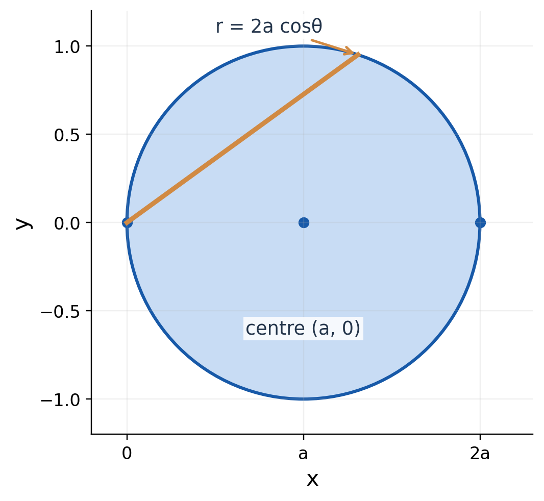
A = ∫[−π/2,π/2] ∫[0,2a cos θ] r dr dθ.
A = 2a²∫[−π/2,π/2] cos²θ dθ = πa².
Worked Example 2.27 – Integrate x over the Shifted Disk
The integrand becomes r cos θ. Therefore:
I = ∫[−π/2,π/2] ∫[0,2a cos θ] r² cos θ dr dθ.
I = (8a³/3)∫[−π/2,π/2] cos⁴θ dθ.
Using the angular integral 3π/8:
I = πa³.
This also equals area times the centroid’s x-coordinate: (πa²)a. The agreement checks both the radial power and angular interval.
Why a Full Turn Is Wrong
For angles with cos θ<0, the proposed upper radius 2a cos θ is negative. Integrating across those angles with ordinary nonnegative-radius bounds would not describe the disk.
Another Valid Substitution
Translate first: x=a+u, y=v. The domain becomes u²+v²≤a² and the translation has Jacobian one. Polar coordinates in (u,v) give the same answer.
Coordinate Choice
Choose coordinates for the boundary and the integrand together. A translated polar system can be simpler than polar coordinates about the original origin.
13. Area Through Double Integrals
The area of a plane region is the integral of 1 over that region. Cartesian and polar formulas are two coordinate descriptions of the same geometric quantity.
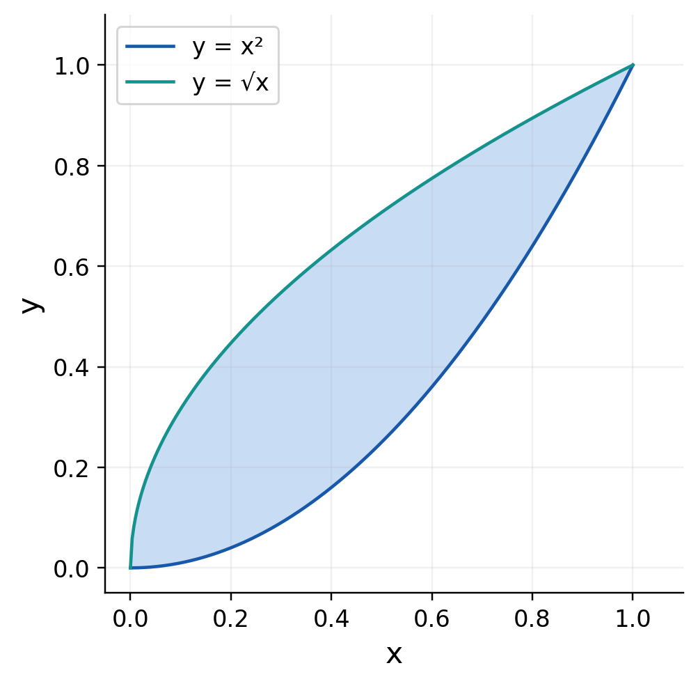
Worked Example 2.28 – Area Between Two Parabolas
In the first quadrant, y=x² and x=y² intersect at (0,0) and (1,1). Solving x=y² for y gives y=√x.
A = ∫[0,1] ∫[x²,√x] 1 dy dx.
A = ∫[0,1] (√x−x²) dx = 1/3.

Worked Example 2.29 – Ellipse Area
Let D satisfy x²/a²+y²/b²≤1, where a,b>0. Set x=au and y=bv. The unit disk in (u,v) maps to the ellipse, with absolute Jacobian ab.
A = ab ∬_(u²+v²≤1) 1 du dv = πab.
Equivalently use x=ar cos θ, y=br sin θ, whose area factor is ab r.
Worked Example 2.30 – Elliptic Quadratic
For the same ellipse:
I = ∬_D (x²/a²+y²/b²) dA.
I = ab ∫[0,2π] ∫[0,1] r³ dr dθ = πab/2.
The average of the scaled quadratic over the filled ellipse is 1/2. It is not 1, because the boundary value is not the value at every interior point.
Area Is Always Nonnegative
If an area calculation is negative, investigate reversed bounds or a missing absolute Jacobian. A signed iterated integral can be negative, but it cannot then represent the intended geometric area.
Scaling Check
Changing a→2a and b→3b multiplies the ellipse area by 6. The transformed area element must reflect both stretches.
14. Volume as Height Times Area
When a solid lies between z=lower(x,y) and z=upper(x,y) above D, its volume is:
V = ∬_D [upper−lower] dA.
First find where the upper surface is actually above the lower one. Their intersection often determines the boundary of D.
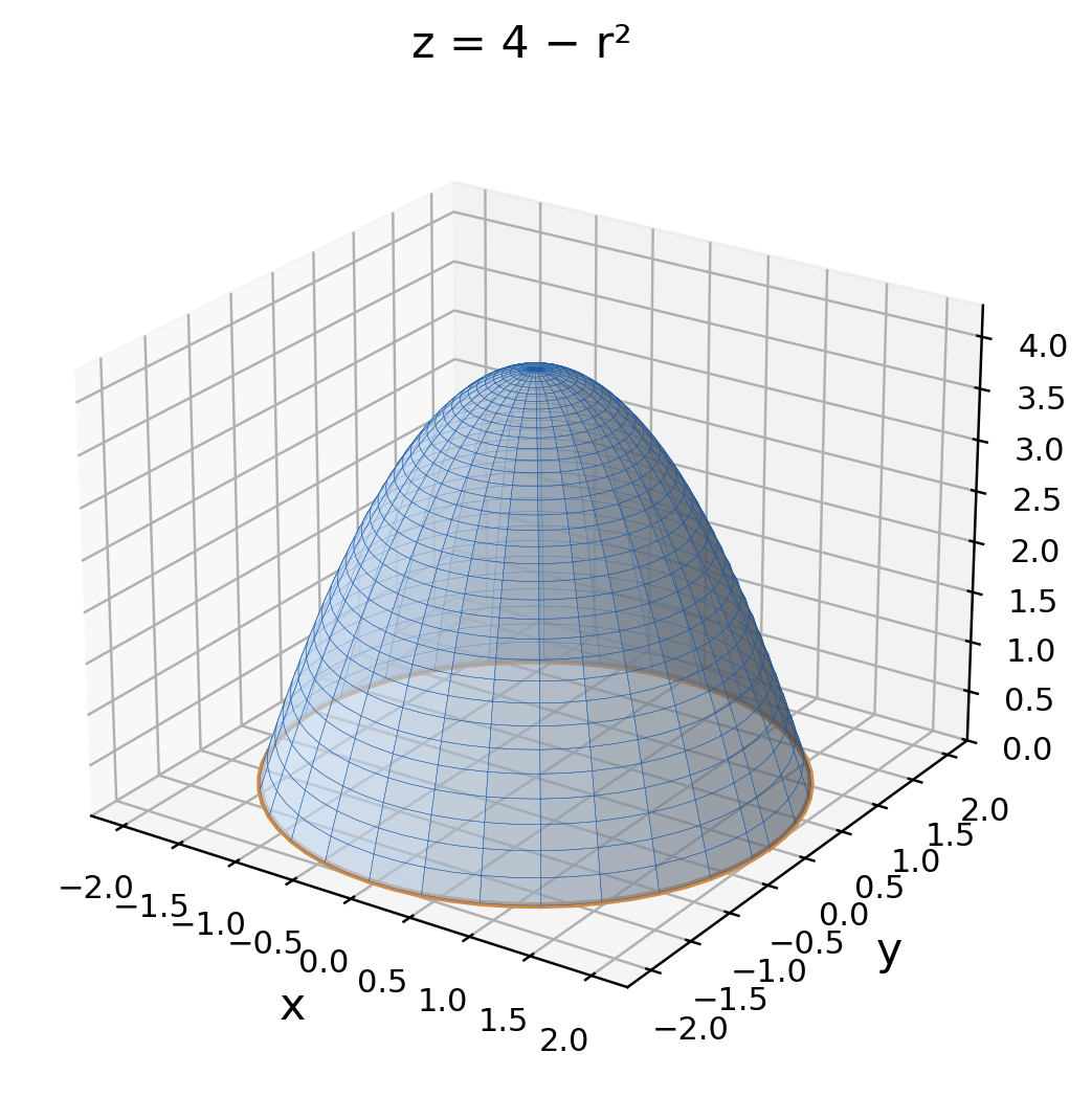
Worked Example 2.31 – A Paraboloid Cap
Find the volume below z=4−x²−y² and above z=0. The height is nonnegative over the disk r≤2.
V = ∫[0,2π] ∫[0,2] (4−r²)r dr dθ.
V = 2π[2r²−r⁴/4] evaluated from r=0 to r=2 = 8π.

Worked Example 2.32 – Two Paraboloids
Let the lower surface be z=x²+y² and the upper surface be z=2−x²−y².
Their intersection satisfies r²=2−r², giving r=1. The vertical height is 2−2r², hence:
V = ∫[0,2π] ∫[0,1] (2−2r²)r dr dθ.
V = 2π[r²−r⁴/2] evaluated from r=0 to r=1 = π.
The height is 2 at the centre and zero at the rim. A cylinder with the same base and maximum height has volume 2π, so π is plausible.
Worked Example 2.33 – Under an Inclined Plane
Over 0≤x≤1, 0≤y≤2, let z=1+x+y. The lower surface is z=0.
V = ∫[0,1] ∫[0,2] (1+x+y) dy dx = 5.
This is an actual volume because the height is positive throughout the base. If a plane crossed below z=0, the base would need restriction or the height difference would need careful interpretation.
Volume Method
Find the projected region, write upper minus lower, check the sign at an interior point, and only then select coordinates.

15. Average Values and Lamina Mass
The average value of an integrable function over a region with area A>0 is:
f_avg = (1/A)∬_D f dA.
A lamina with nonnegative areal mass density ρ has total mass M=∬_D ρ dA. Its density-weighted centre is obtained from first moments.
x̄ = (∬_D xρ dA)/M, ȳ = (∬_D yρ dA)/M.
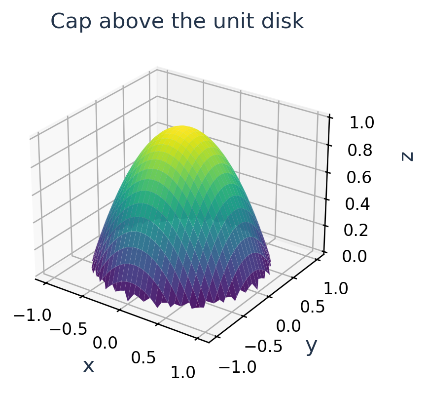
Worked Example 2.34 – Average Radial Height
For f=4−r² over a disk r≤2, the integral is 8π and the area is 4π. Therefore the average height is 2.
The average is between the minimum 0 and maximum 4, as it must be.
Worked Example 2.35 – Mass and Centroid
Let D be x≥0, y≥0, x+y≤1, with density ρ=x+y. Units are chosen consistently.
M = ∫[0,1] ∫[0,1−x] (x+y) dy dx = 1/3.
By interchange symmetry, the x and y moments are equal. The x-coordinate moment is:
M_y = ∬_D (x²+xy) dA.
M_y = 1/12 + 1/24 = 1/8.
Thus:
x̄ = ȳ = (1/8)/(1/3) = 3/8.
The density is larger near the sloping edge, so the centroid moves away from the origin compared with the uniform triangle’s centroid (1/3,1/3).


Distinguish Averages
An area average divides by area. A mass-weighted average divides by total mass and includes density in the numerator. These are equal only in suitable constant-density cases.
16. General Change of Variables
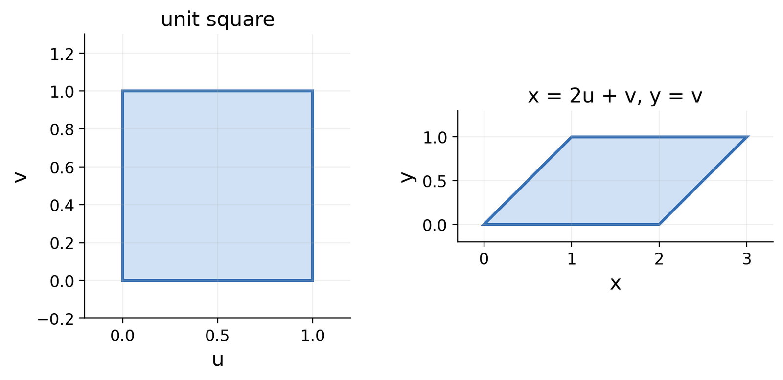
Let x=x(u,v), y=y(u,v) map a simpler region S to D. For a smooth one-to-one transformation with a nonzero Jacobian in the interior:
∬_D f(x,y) dA = ∬_S f(x(u,v),y(u,v)) |J| du dv.
J = ∂(x,y)/∂(u,v) = xᵤyᵥ−xᵥyᵤ.
The absolute value measures local area magnification. The sign of J records orientation and cannot make physical area negative.

What Must Be Transformed
- The integrand, including every occurrence of x and y.
- All region boundaries.
- The differential element using the absolute Jacobian.
Choosing a Useful Substitution
Parallel boundary pairs often suggest linear variables such as u=x+y and v=x−y. Hyperbolas may suggest products or ratios. Circles suggest polar coordinates.
Worked Example 2.36 – A Pure Scaling
For x=2u, y=3v, the Jacobian is 6. A unit square becomes a rectangle of area 6.
∬_D (x+y) dA = 6∫[0,1] ∫[0,1] (2u+3v) dv du = 15.
A direct calculation over 0≤x≤2, 0≤y≤3 gives the same answer.
Direct Versus Inverse Jacobian
If the easy derivatives give ∂(u,v)/∂(x,y), then invert the determinant where it is nonzero:
|∂(x,y)/∂(u,v)| = 1/|∂(u,v)/∂(x,y)|.
Do not use both the direct and inverse factors. Exactly one area conversion belongs in the transformed integral.
Validity Check
A nonzero local determinant does not by itself guarantee a globally one-to-one map. Choose a domain or split it so that the same point is not counted repeatedly.
17. Linear Transformation Example
Worked Example 2.37 – A Parallelogram Integral
Let D be bounded by x+y=0, x+y=2, x−y=0 and x−y=2. Set:
u = x+y, v = x−y.
The new region is the square 0≤u≤2, 0≤v≤2. Inverting:
x = (u+v)/2, y = (u−v)/2, |J| = 1/2.


Its vertices are (0,0), (1,1), (2,0), (1,−1), and its area is 2.
Checking the Inverse Determinant
From x=(u+v)/2 and y=(u−v)/2, the derivative matrix has first row (1/2,1/2) and second row (1/2,−1/2). Its determinant is −1/4−1/4=−1/2.
The forward determinant of u=x+y, v=x−y is −2. Their product is one, as required for inverse transformations. This check confirms the reciprocal relationship without relying on a memorised area factor.
Transform the Function Too
Evaluate x²−y² over D. Since x²−y²=(x+y)(x−y)=uv:
I = (1/2)∫[0,2] ∫[0,2] uv dv du.
I = (1/2)(2²/2)² = 2.
Worked Example 2.38 – Integrate x
I = ∫[0,2] ∫[0,2] (u+v)/4 dv du = 2.
The parallelogram has area 2 and centroid (1,0), so the integral of x is 2. This independently checks the factor 1/2.
Orientation Does Not Change Area
The signed determinant is −1/2. It is negative because the transformation reverses orientation. The integral uses +1/2. Using −1/2 would incorrectly produce negative area and reverse both positive answers.
Boundary Verification
The corner (u,v)=(2,0) maps to (1,1). The corner (0,2) maps to (1,−1). Mapping all corners is a quick way to catch a wrong inverse formula.
Memory Aid
Transform the boundary equations before the integrand. A rectangular uv-domain is the main reason this substitution helps.
18. A Nonlinear Product-Ratio Map
Worked Example 2.39 – Hyperbolic Region
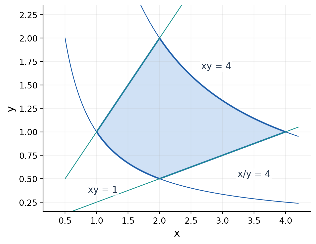
In the first quadrant let 1≤xy≤4 and 1≤x/y≤4. Choose u=xy and v=x/y. The new domain is 1≤u≤4, 1≤v≤4.
The positivity restriction gives a single inverse branch:
x = √(uv), y = √(u/v).
The forward determinant is:
∂(u,v)/∂(x,y) = −2x/y = −2v.
|J| = 1/(2v).

Boundary Images
The curve xy=1 becomes u=1, while xy=4 becomes u=4. The lines x=y and x=4y become v=1 and v=4. Four curved or sloping boundaries have become the four sides of a rectangle.
This is why the substitution helps: the region simplifies even though the inverse formulas contain square roots. The integrand xy also becomes the single variable u.
Evaluate the Transformed Integral
For integrand xy=u:
I = ∫[1,4] ∫[1,4] u/(2v) dv du.
I = (1/2)([u²/2] evaluated from 1 to 4)([ln v] evaluated from 1 to 4).
I = (15/4)ln 4.
Worked Example 2.40 – Region Area
Set the integrand to 1:
A = ∫[1,4] ∫[1,4] 1/(2v) dv du = (3/2)ln 4.
The average xy over this region is I/A=5/2. This lies between its minimum 1 and maximum 4.
Why the Quadrant Matters
Without the first-quadrant restriction, the equations u=xy>0 and v=x/y>0 also allow both x and y negative. The positive square-root inverse would cover only one of those components.
A substitution must specify the region and the inverse branch together. Multiple branches may require separate integrals or a multiplicity factor justified from the geometry.
Final Check
The ratio v is dimensionless when x and y share units. The factor 1/(2v) is positive on the chosen rectangle, and the resulting integral is positive.
19. Triple Integrals on Boxes
A triple integral sums f times small volume elements. For a rectangular box and a continuous function, integrate successively in any chosen order.
∭_E f dV = ∫[a,b] ∫[c,d] ∫[p,q] f dz dy dx.
With dz innermost, hold x and y fixed until the z-limits have been inserted. Then integrate the remaining y-expression and finally x.

Worked Example 2.41 – Box Volume
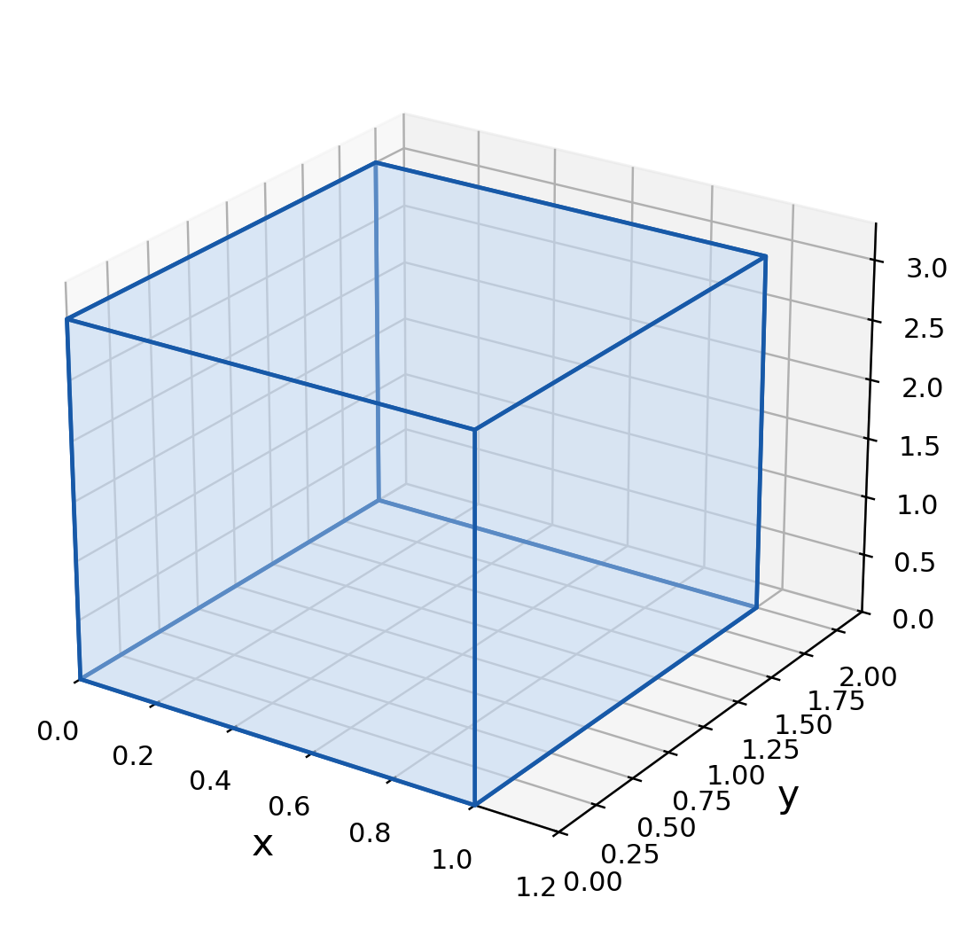
V = ∫[0,1] ∫[0,2] ∫[0,3] 1 dz dy dx = 6.
The differential element dx dy dz has units of volume, regardless of integration order.
Worked Example 2.42 – A Product Integrand
Evaluate xyz over the same box. Both region and function separate:
I = (∫[0,1] x dx)(∫[0,2] y dy)(∫[0,3] z dz).
I = (1/2)(2)(9/2) = 9/2.
Worked Example 2.43 – A Sum Integrand
For x+y+z, use linearity. The average coordinates of the box are 1/2, 1 and 3/2, so the average sum is 3. Multiplying by volume 6 predicts 18.
Directly, the z-integration gives 3x+3y+9/2. The y-integration gives 6x+15, and the final x-integral is 18.
Avoid an Invalid Product Shortcut
A function such as x+y+z is a sum, not a product. Its triple integral is a sum of three separable terms; it is not the product of three one-variable integrals of x+y+z.
Variable Check
After integrating z, no free z should remain. After integrating y, no free y should remain. A final definite triple integral is a number unless parameters were part of the problem.
20. Tetrahedral Bounds
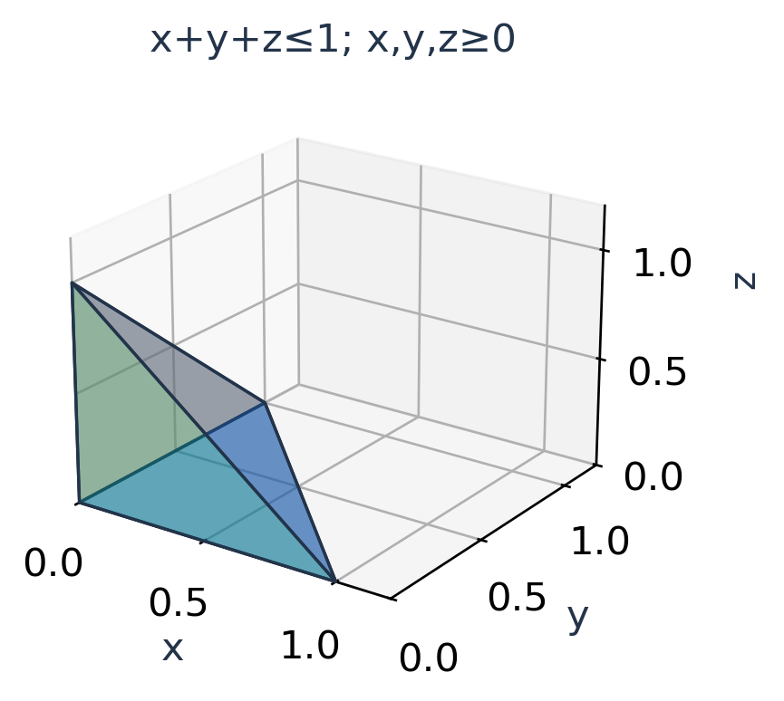
A solid in the first octant below the plane x+y+z=a, a>0, has inequalities x,y,z≥0 and x+y+z≤a.
Project onto the xy-plane: x≥0, y≥0, x+y≤a. Above each projected point, z runs from 0 to a−x−y.
∭_E f dV = ∫[0,a] ∫[0,a−x] ∫[0,a−x−y] f dz dy dx.


Worked Example 2.44 – Volume
Integrating 1 first in z gives a−x−y. Integrating in y then gives (a−x)²/2.
V = (1/2)∫[0,a] (a−x)² dx = a³/6.
Worked Example 2.45 – Integrate x
For the unit tetrahedron:
I = ∫[0,1] ∫[0,1−x] ∫[0,1−x−y] x dz dy dx.
I = (1/2)∫[0,1] x(1−x)² dx = 1/24.
Its volume is 1/6, so the uniform mean x-coordinate is (1/24)/(1/6)=1/4. By symmetry, the y and z means are also 1/4.
Worked Example 2.46 – Sum of Coordinates
For x+y+z over the same tetrahedron, symmetry gives three identical integrals:
∭_E (x+y+z) dV = 3(1/24) = 1/8.
Why All Bounds Cannot Be 0 to 1
The cube 0≤x,y,z≤1 contains many points above the plane, such as (1,1,1). The tetrahedron occupies only one-sixth of the unit cube’s volume.
Bound Order
For dz dy dx, the z-bound can use x and y; the y-bound can use x; the x-bound is constant. Writing y≤1−x−z while z is already integrated would make the order inconsistent.
Projection Method
Describe the vertical segment first, then its two-dimensional base. This turns a three-dimensional bounds problem into a familiar double-integral region.

21. Changing Order in a Solid
The same solid may admit several useful orders. Each order requires an appropriate projection and inner segment.
Worked Example 2.47 – An Ordered Wedge
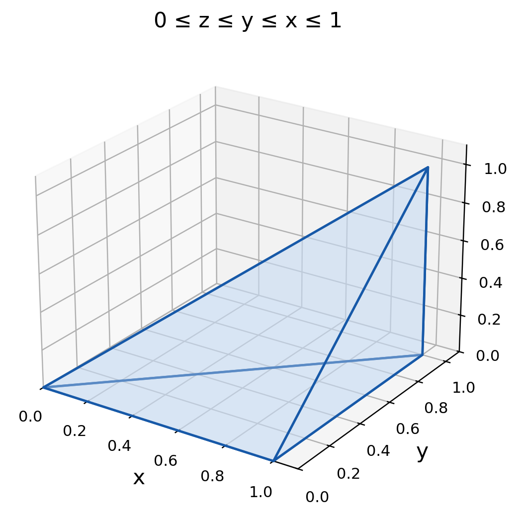
Let E satisfy 0≤z≤y≤x≤1. A natural order is:
∫[0,1] ∫[0,x] ∫[0,y] f(x,y,z) dz dy dx.
To integrate x first, fix y and z. Then y≤x≤1. The yz-projection has 0≤z≤y≤1, giving:
∫[0,1] ∫[z,1] ∫[y,1] f(x,y,z) dx dy dz.

Worked Example 2.48 – Volume of the Wedge
Original order:
V = ∫[0,1] ∫[0,x] y dy dx.
V = (1/2)∫[0,1] x² dx = 1/6.
Reversed order:
V = ∫[0,1] ∫[z,1] (1−y) dy dz.
V = ∫[0,1] (1/2−z+z²/2) dz = 1/6.
The unit cube splits into six equal pieces corresponding to the six possible strict orderings of x,y,z. This symmetry explains the volume 1/6.
Worked Example 2.49 – Integrate z
Original order gives:
I = ∫[0,1] ∫[0,x] y²/2 dy dx = 1/24.
The mean z is therefore 1/4, the mean minimum of the three ordered uniform coordinates on this geometric region.
Reordering Habit
Start from inequalities, not from the appearance of the old integral. Test an interior point such as (3/4,1/2,1/4) in every proposed description.
22. Cylindrical Coordinates
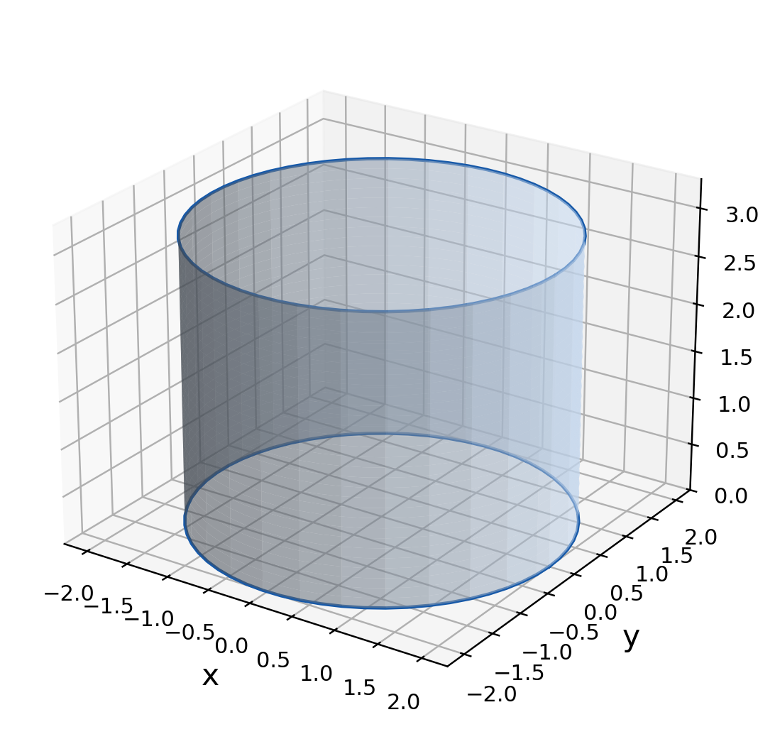
Cylindrical coordinates use polar coordinates in the xy-plane and retain z:
x = r cos θ, y = r sin θ, z = z.
dV = r dz dr dθ.
They are useful for cylinders, cones and surfaces described by x²+y².

Worked Example 2.50 – Cylinder Volume
V = ∫[0,2π] ∫[0,2] ∫[0,3] r dz dr dθ = 12π.
This matches base area 4π times height 3.
Worked Example 2.51 – An Upper Half-Cylinder
For x²+y²≤4, y≥0 and 0≤z≤3, use the angular interval 0≤θ≤π, not a full turn.
V = ∫[0,π] ∫[0,2] ∫[0,3] r dz dr dθ = 6π.
This is half the full cylinder volume. The radial and height bounds stay the same; only the azimuth interval changes.
Worked Example 2.52 – Radial Density
Let a cylinder have radius a and height h, with density ρ=x²+y²=r². Then:
M = ∫[0,2π] ∫[0,a] ∫[0,h] r³ dz dr dθ.
M = πha⁴/2.
The density-weighted centre lies on the z-axis by rotational symmetry and at height h/2 because density does not depend on z.
Worked Example 2.53 – Cylinder Below a Plane
For r≤1, 0≤z≤2+x, the height becomes 2+r cos θ. It stays positive because x≥−1.
V = ∫[0,2π] ∫[0,1] (2+r cos θ)r dr dθ.
The cos θ term integrates to zero over a full turn, leaving V=2π. This equals disk area times the mean height 2.
Avoid Double Jacobians
The z-integration contributes the vertical height; the cylindrical coordinate conversion contributes r. Multiplying by another r because the region looks circular would count the area scale twice.
Choose Cylindrical When
The boundary contains x²+y², the angular range is simple, and z is naturally bounded between two surfaces over a circular base.


23. Spherical Coordinates
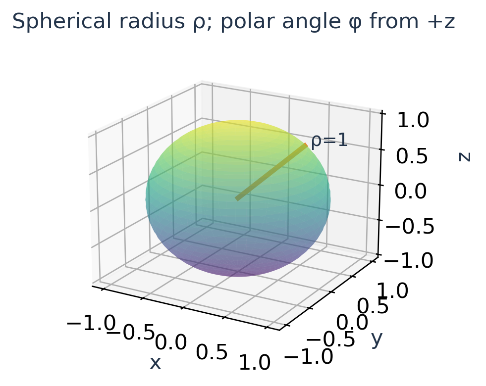
Use ρ for distance from the origin, θ for azimuth around the z-axis and φ for angle measured down from the positive z-axis:
x = ρ sin φ cos θ, y = ρ sin φ sin θ.
z = ρ cos φ, dV = ρ² sin φ dρ dφ dθ.
For a full ball, 0≤ρ≤a, 0≤φ≤π and 0≤θ≤2π.

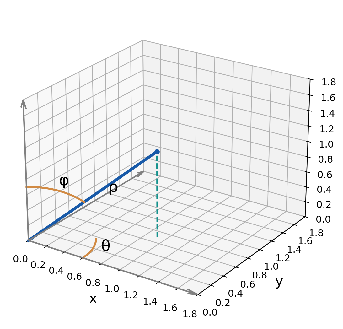
The two angular variables have different roles. Always define the convention because some texts interchange their names.
Convert Standard Boundaries
The sphere x²+y²+z²=a² becomes ρ=a. The plane z=0 corresponds to φ=π/2. The positive z-axis is φ=0.
A lower half-ball uses π/2≤φ≤π. Because sin φ remains nonnegative throughout 0≤φ≤π, the standard spherical volume element stays nonnegative on both halves.
Worked Example 2.54 – Ball Volume
V = ∫[0,2π] ∫[0,π] ∫[0,a] ρ² sin φ dρ dφ dθ.
V = 2π × 2 × a³/3 = 4πa³/3.
Worked Example 2.55 – Radial Quadratic
Evaluate x²+y²+z² over the ball. The integrand becomes ρ², so:
I = ∫[0,2π] ∫[0,π] ∫[0,a] ρ⁴ sin φ dρ dφ dθ.
I = 4πa⁵/5.
The average squared radius is I/V=3a²/5. It is smaller than the boundary value a² because the integral includes the entire interior.
Octant Restriction
For the first octant, both θ and φ run from 0 to π/2. A radial integrand contributes one-eighth of its full-ball integral.
Spherical Check
The volume element has ρ² sin φ. Omitting sin φ or using only one power of ρ cannot reproduce the known sphere volume.
Worked Example 2.56 – A Spherical Shell
For a≤ρ≤b with 0<a<b, subtract the inner ball:
V = 4π∫[a,b] ρ² dρ = (4π/3)(b³−a³).
The shell volume depends on a difference of cubes, not the cube of the thickness b−a. A thin outer layer surrounds a large area, so radius and thickness play different roles.

24. A Sphere Intersected by a Cone
A cone z=√(x²+y²) has z=r in cylindrical coordinates. In spherical coordinates, ρ cos φ=ρ sin φ, so its upper-half opening is φ=π/4.
Worked Example 2.57 – Inside a Sphere, Above a Cone
Let E be inside x²+y²+z²≤a² and above z=√(x²+y²). The bounds are:
0≤ρ≤a, 0≤φ≤π/4, 0≤θ≤2π.

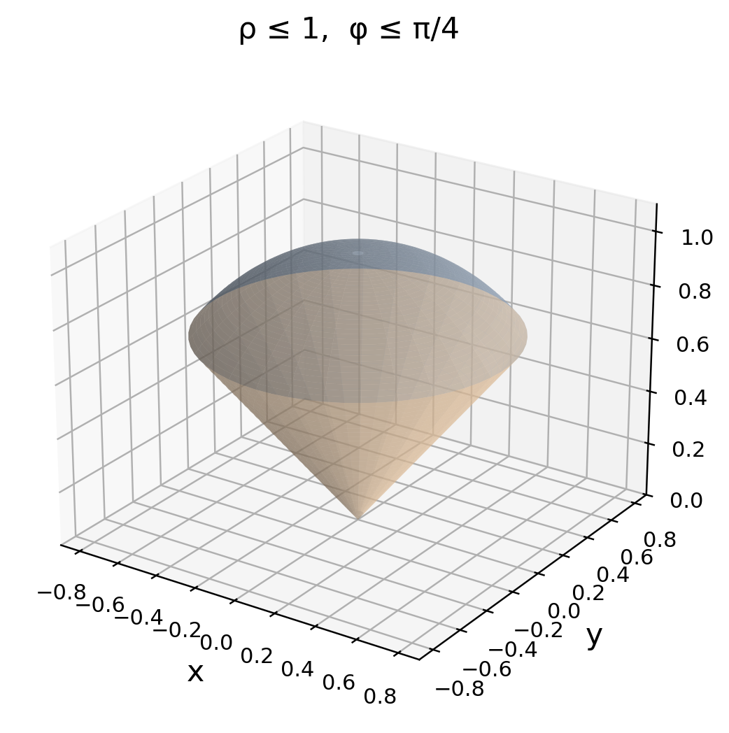
V = (2πa³/3)(1−1/√2).
This follows by multiplying a³/3 by the azimuth integral 2π and the polar-angle integral 1−cos(π/4).
A Solid-Angle Interpretation
The angular factor measures the fraction of directions included by the cone. For an opening angle α measured from +z:
Ω = ∫[0,2π] ∫[0,α] sin φ dφ dθ = 2π(1−cos α).
Multiplying this angular factor by a³/3 gives the volume inside the radius-a ball in those directions. At α=π/2 it gives a hemisphere; at α=π it gives the full ball.
Worked Example 2.58 – Integrate z
With z=ρ cos φ:
I = ∫[0,2π] ∫[0,π/4] ∫[0,a] ρ³ sin φ cos φ dρ dφ dθ.
I = 2π × (a⁴/4) × (1/4) = πa⁴/8.
The result is positive because z≥0 throughout E. Its units are length⁴, as expected for z times volume.
Which Angle Describes the Cone?
The cone is not θ=π/4. That would be a vertical half-plane at one azimuth. A rotationally symmetric cone keeps φ fixed while θ makes a complete turn.
Compare with a Spherical Cap
The condition z≥a/2 gives ρ cos φ≥a/2. It is a horizontal plane cut and does not produce the same constant φ-bound with ρ starting from zero.
Geometry First
Cones through the origin often become constant-angle boundaries. Spheres centred at the origin become constant-radius boundaries. Plane cuts usually need coupled bounds.
25. Triple Integrals Between Surfaces
A useful general form is:
∭_E f dV = ∬_D ∫[z₁(x,y),z₂(x,y)] f dz dA.
The xy-projection D is where z₂≥z₁. For f=1 the inner integral is upper minus lower, reproducing the double-integral volume formula.
Worked Example 2.59 – Paraboloid to Plane
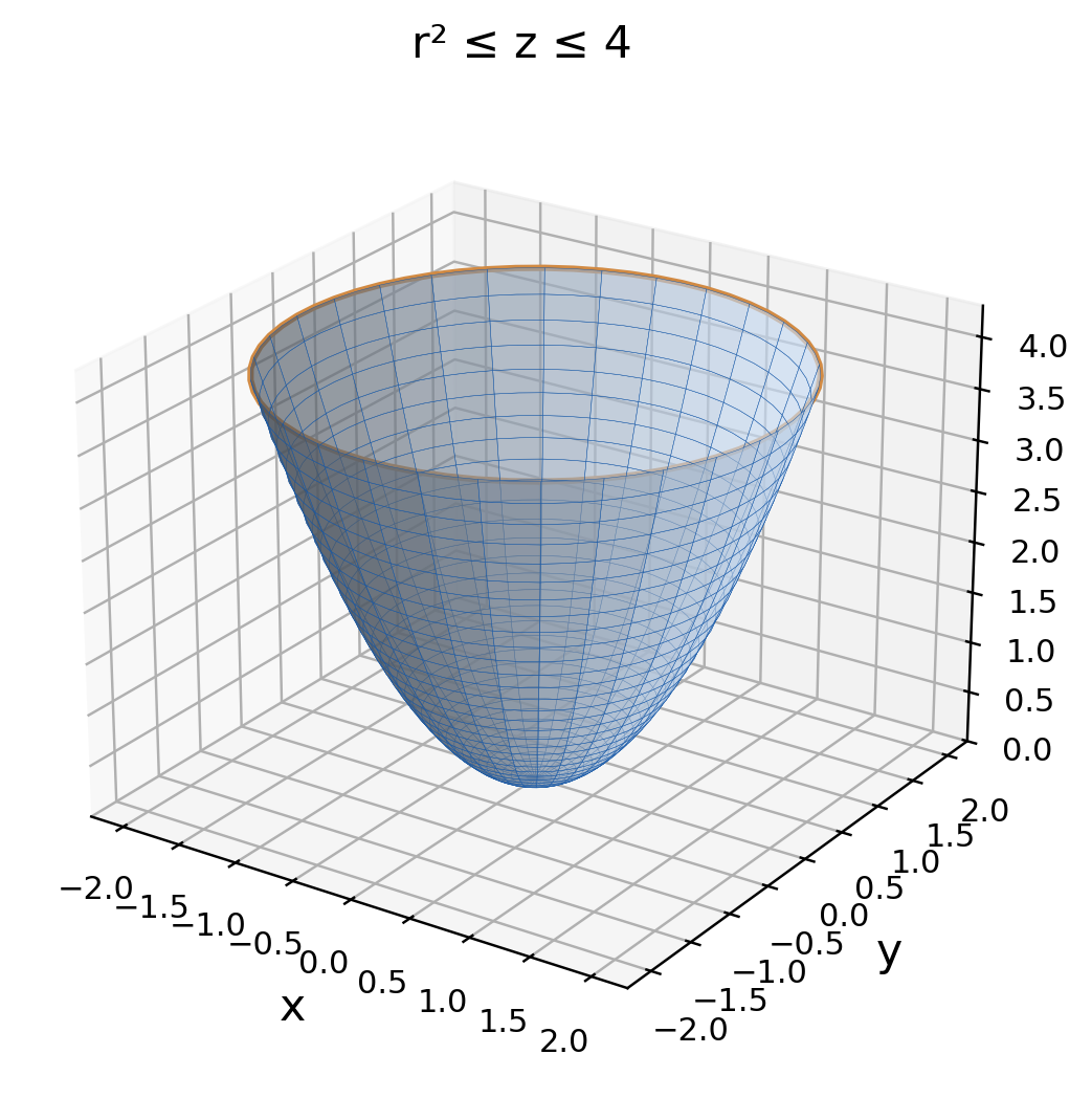
Let r²≤z≤4. Their intersection is r=2, so use 0≤r≤2.
V = ∫[0,2π] ∫[0,2] ∫[r²,4] r dz dr dθ.
V = ∫[0,2π] ∫[0,2] (4−r²)r dr dθ = 8π.

Worked Example 2.60 – Integrate z
M_xy = ∫[0,2π] ∫[0,2] ∫[r²,4] zr dz dr dθ.
The inner integral is r(16−r⁴)/2. Therefore:
M_xy = π∫[0,2] (16r−r⁵) dr = 64π/3.
For uniform density, the centre height is:
z̄ = (64π/3)/(8π) = 8/3.
It lies between the bottom height 0 and top height 4 and is above the mid-height 2 because higher horizontal slices have greater area.
Alternative Slicing Check
At fixed z in [0,4], the solid has r≤√z, so its horizontal cross-section is a disk of area πz. Thus:
V = ∫[0,4] πz dz = 8π.
M_xy = ∫[0,4] z(πz) dz = 64π/3.
Both approaches agree. Choosing horizontal slices makes this particular check especially short.
Coordinate Judgement
The best coordinate system and the best integration order are separate choices. Even in cylindrical coordinates, either z or r may be the easiest inner variable.
26. The Gamma Function
The Gamma function extends the factorial pattern through an improper integral. For real s>0:
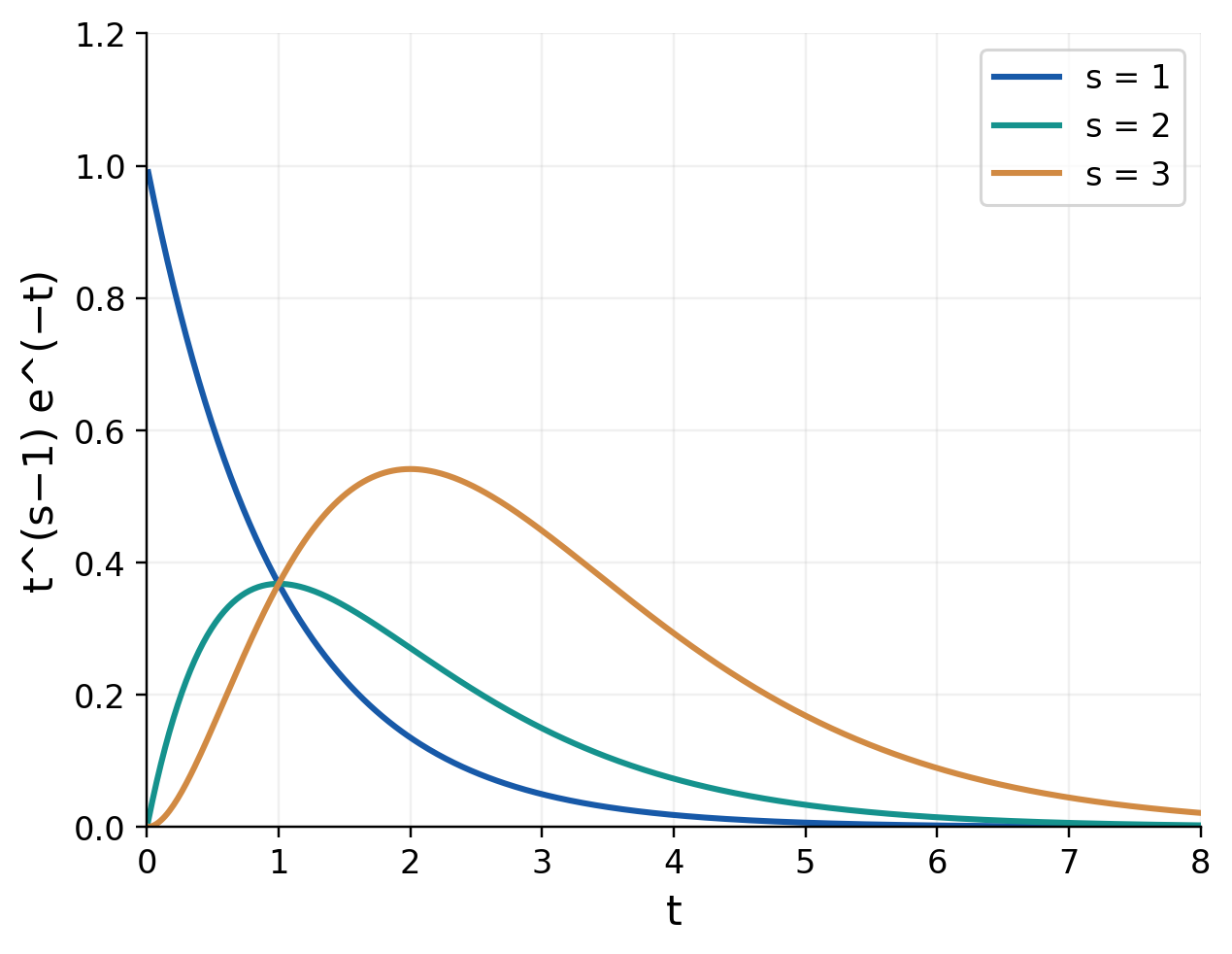
Γ(s) = ∫[0,∞] t^(s−1)e^(−t) dt.
There are two convergence questions. Near zero, t^(s−1) is integrable precisely when s>0. At infinity the exponential decay dominates every fixed real power.

Why a Special Function Is Useful
Many definite integrals do not have convenient elementary antiderivatives. Recognising a Gamma pattern gives a standard exact value and a systematic way to simplify it.
Improper-Integral Notation
The definition means a limit at infinity and, when needed, another at zero. Split at any fixed positive point such as 1. Both pieces must converge.
For s=1/2 the near-zero behaviour is t^(−1/2), whose integral from zero to one is 2. This comparison establishes convergence there even though the integrand has no finite endpoint value.
Reading the Parameter Correctly
In t^(s−1)e^(−t), the exponent is s−1. If the power is t⁴, the parameter is 5, not 4.
Worked Example 2.61 – The First Value
Γ(1) = ∫[0,∞] e^(−t) dt = 1.
Insert an upper limit R and take R→∞. Since e^(−R)→0, the result is 1.
Worked Example 2.62 – A Convergent Fractional Power
∫[0,∞] t^(−1/2)e^(−t) dt = Γ(1/2).
Although the integrand becomes unbounded at zero, the singularity is integrable because the exponent −1/2 is greater than −1. Unbounded does not automatically mean divergent.
A Divergent Case
For s=0, the integrand is e^(−t)/t. Near zero it behaves like 1/t, whose integral diverges. The displayed defining integral therefore does not apply at s=0.
Parameter Check
Identify the power, add one to find s, then verify s>0 before using the real integral definition. Analytic continuation is not needed in this unit.
Worked Example 2.63 – A Nonconvergent Power
Consider t^(−3/2)e^(−t) near zero. For 0<t<1, e^(−t)≥e^(−1), so the integrand is at least e^(−1)t^(−3/2).
The comparison integral diverges. Thus the proposed half-line integral is not a finite Gamma integral under this unit’s real definition. Check the lower endpoint before using a symbol Γ(s).
27. Gamma Recurrence and Factorials
Integrate the defining integral for Γ(s+1) by parts, taking u=tˢ and dv=e^(−t)dt. For s>0, the boundary term vanishes at both endpoints.
Γ(s+1) = sΓ(s).
Since Γ(1)=1, repeated use gives:
Γ(n+1) = n!, n=0,1,2,…
Equivalently, Γ(n)=(n−1)! for a positive integer n. This one-step shift is a frequent source of errors.


Worked Example 2.64 – A Simple Exponential Moment
For the integral of t e^(−t), the parameter is s=2:
∫[0,∞] te^(−t) dt = Γ(2) = 1.
Integration by parts gives the same value. The recurrence is a compact way to repeat that calculation for higher integer powers without redoing every antiderivative.
Worked Example 2.65 – Integer Argument
Γ(6) = 5Γ(5) = 5×4×3×2×1 = 120.
Worked Example 2.66 – A Definite Integral
I = ∫[0,∞] t⁴e^(−t) dt = Γ(5) = 24.
Worked Example 2.67 – Ratio of Gamma Values
For s>0:
Γ(s+3)/Γ(s) = s(s+1)(s+2).
At s=2 this equals 2×3×4=24, consistent with Γ(5)/Γ(2)=24/1.
Boundary-Term Justification
As t→∞, tˢe^(−t)→0. As t→0+, tˢ→0 for s>0. Both facts are needed to discard the integration-by-parts boundary term.
If s were nonpositive, the same argument could not simply be copied into the defining integral.
Memory Trick
Gamma’s argument is one more than the factorial index: Γ(6)=5!, Γ(5)=4!, Γ(1)=0!. Write the intermediate factorial before calculating.
28. Half-Integer Gamma Values
The key starting value is:
Γ(1/2) = √π.
A double-integral proof is given in the Gaussian-integral section. Once this value is known, the recurrence produces all positive half-integer values.
Γ(3/2) = √π/2.
Γ(5/2) = 3√π/4.
Γ(7/2) = 15√π/8.
For an integer n≥0:
Γ(n+1/2) = [(2n)!/(4ⁿn!)]√π.
The formula includes n=0 and reduces to √π.
Why the Factorial Expression Holds
The recurrence multiplies the odd integers 1,3,5,…,2n−1 and divides by 2 at each of n steps.
In (2n)!, the even factors multiply to 2ⁿn!, leaving the odd-factor product (2n)!/(2ⁿn!). Dividing by the additional 2ⁿ gives the stated denominator 4ⁿn!. This derivation also confirms the formula at n=0.
Worked Example 2.68 – A Larger Half-Integer
Γ(9/2) = (7/2)(5/2)(3/2)(1/2)√π = 105√π/16.
Do not multiply by 9/2 at the first step; Γ(9/2)=(7/2)Γ(7/2).
Worked Example 2.69 – Fractional-Power Integral
I = ∫[0,∞] t^(3/2)e^(−t) dt.
Match s−1=3/2, so s=5/2:
I = Γ(5/2) = 3√π/4.
Worked Example 2.70 – A Ratio
Γ(7/2)/Γ(3/2) = [(15/8)√π]/[(1/2)√π] = 15/4.
The √π factor cancels. Recognising recurrence before decimal evaluation keeps the answer exact and avoids rounding error.
Self-Check
Γ(1/2)≈1.772, Γ(3/2)≈0.886 and Γ(5/2)≈1.329. Gamma need not increase between every pair of small positive arguments.
Worked Example 2.71 – Another Convergent Singularity
∫[0,∞] t^(−1/2)e^(−4t) dt = 4^(−1/2)Γ(1/2) = √π/2.
The substitution u=4t contributes a factor 1/4, while t^(−1/2) contributes 2. Their combined scale is 1/2. Retaining both factors is essential for a correct fractional-power substitution.
29. Scaled Gamma-Type Integrals
Substitution converts many exponential integrals to the defining Gamma integral. For a>0, k>0 and m>0:
∫[0,∞] x^(m−1)e^(−axᵏ) dx = (1/k)a^(−m/k)Γ(m/k).
To derive it, set t=axᵏ. The differential and power combine as:
x^(m−1) dx = (1/k)a^(−m/k)t^(m/k−1) dt.
The endpoints remain 0 and infinity. The positivity conditions ensure convergence and a real positive substitution.

Scale Behaviour
For fixed m and k, increasing a makes the exponential decay faster. The integral decreases as a^(−m/k), exactly as the formula predicts.
Doubling a therefore multiplies the integral by 2^(−m/k). This is a useful check when a substitution produces several powers of a: the final power must be negative for positive m and k.
Worked Example 2.72 – Scaled Exponential
I = ∫[0,∞] x²e^(−3x) dx.
Here m=3, k=1, a=3:
I = 3^(−3)Γ(3) = 2/27.
Worked Example 2.73 – A Quadratic Exponent
I = ∫[0,∞] x⁴e^(−2x²) dx.
Use m=5, k=2 and a=2:
I = (1/2)2^(−5/2)Γ(5/2) = 3√π/(32√2).
Worked Example 2.74 – Cubic Substitution
∫[0,∞] x⁵e^(−x³) dx = (1/3)Γ(2) = 1/3.
A direct substitution t=x³ gives x⁵dx=(t/3)dt, confirming the same answer.
Pattern Method
Write the integrand as x^(m−1), not xᵐ. Identify a and k from the exponential separately. This prevents a missing factor or a shifted Gamma argument.
30. The Gaussian Integral
Let I be the nonnegative half-line Gaussian integral:
I = ∫[0,∞] e^(−x²) dx.
Its square becomes a double integral over the first quadrant:
I² = ∫[0,∞] ∫[0,∞] e^(−(x²+y²)) dx dy.
The integrand is nonnegative, so the product and order manipulations are justified. Polar coordinates turn the quadrant into r≥0, 0≤θ≤π/2.
I² = ∫[0,π/2] ∫[0,∞] e^(−r²)r dr dθ.
I² = (π/2)(1/2) = π/4.
Since I>0:
I = √π/2.


Connecting Gaussian and Gamma
Set t=x² in Γ(1/2):
Γ(1/2) = ∫[0,∞] t^(−1/2)e^(−t) dt = 2∫[0,∞] e^(−x²) dx = √π.
Worked Example 2.75 – Full-Line Scaling
For a>0:
∫[−∞,∞] e^(−ax²) dx = √(π/a).
The factor two comes from even symmetry; the factor 1/√a comes from u=√a x.
Worked Example 2.76 – A Two-Dimensional Gaussian
∬_(ℝ²) e^(−(x²+y²)) dA = π.
Use r from 0 to infinity and θ from 0 to 2π. The radial integral is 1/2, giving π.
Why the Two Answers Differ
The first-quadrant double integral is π/4. The full-plane double integral is π. Mixing the angular ranges changes the result by a factor of four.
Proof Structure
Square the integral, identify the quadrant, include the polar r, evaluate the radial integral, then take the positive square root.
31. The Beta Function
For real p>0 and q>0:
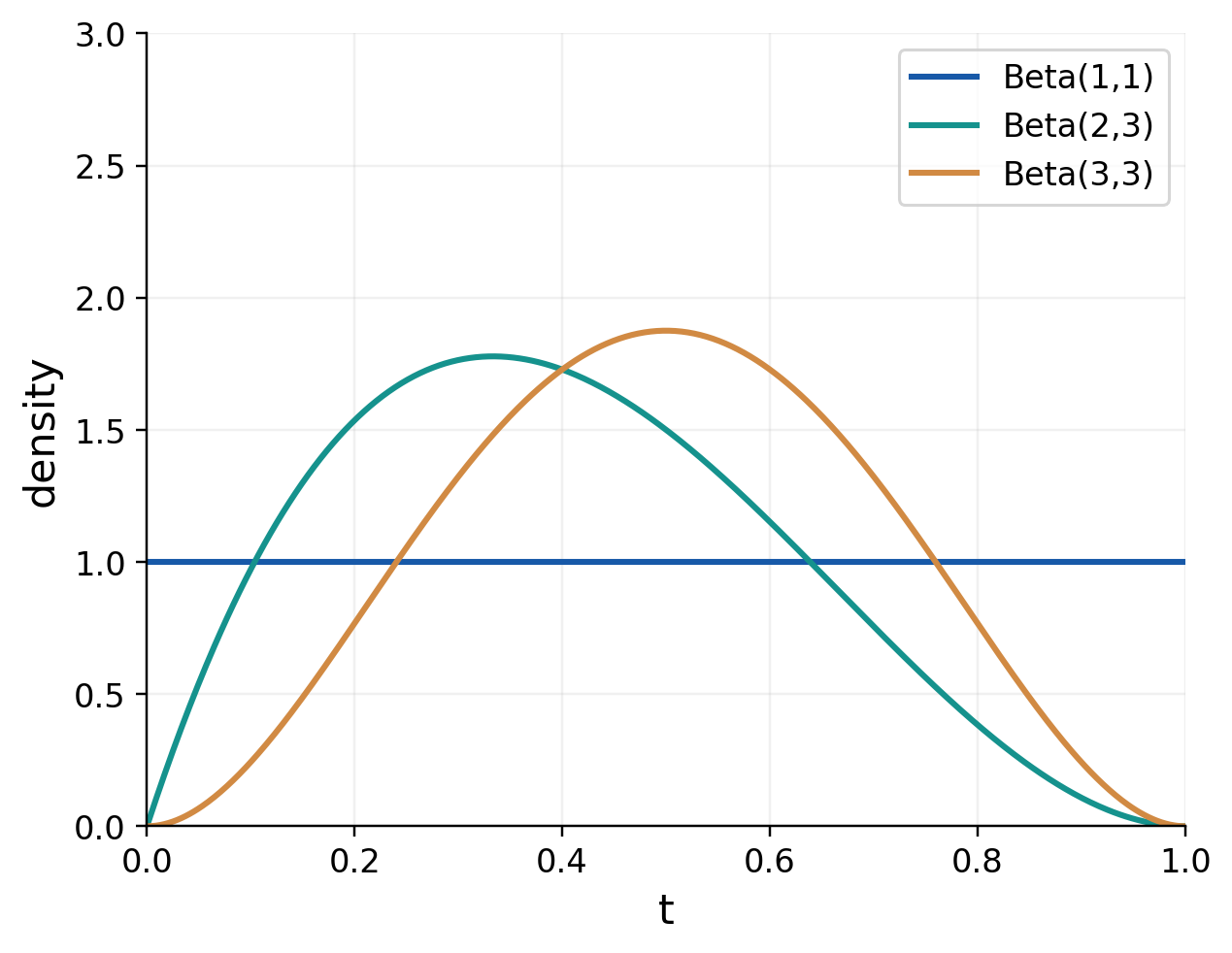
B(p,q) = ∫[0,1] t^(p−1)(1−t)^(q−1) dt.
Near t=0, convergence requires p>0. Near t=1, convergence requires q>0. Both endpoint conditions matter.
The powers are p−1 and q−1. Match them separately rather than reading the exponents as the Beta arguments.

Worked Example 2.77 – Integer Powers
∫[0,1] t²(1−t)³ dt = B(3,4).
The arguments are 3 and 4, not 2 and 3. Evaluation through Gamma functions follows in the next section.
Worked Example 2.78 – One Argument Equals One
For p>0:
B(p,1) = ∫[0,1] t^(p−1) dt = 1/p.
By symmetry B(1,p)=1/p as well.
Worked Example 2.79 – B(2,2)
B(2,2) = ∫[0,1] t(1−t) dt.
B(2,2) = [t²/2−t³/3] evaluated from t=0 to t=1 = 1/6.
Worked Example 2.80 – An Endpoint Singularity
B(1/2,1/2) = ∫[0,1] dt/√(t(1−t)) = π.
With t=sin²θ, the denominator is sin θ cos θ and dt=2sin θ cos θ dθ. The transformed integral is twice the integral of 1 from 0 to π/2, giving π.
The endpoint infinities are integrable. However, replacing either argument by zero produces a divergent endpoint in this real integral definition.
Beta Recognition
A finite interval with powers at both endpoints suggests Beta. A half-line with exponential decay suggests Gamma. Always transform the interval as well as the integrand.
32. Beta–Gamma Relation
For p,q>0:
B(p,q) = Γ(p)Γ(q)/Γ(p+q).
This identity connects two one-dimensional special functions through a two-dimensional change of variables.
Start from the product:
Γ(p)Γ(q) = ∫[0,∞] ∫[0,∞] x^(p−1)y^(q−1)e^(−(x+y)) dx dy.
Use x=ut and y=u(1−t), with u>0 and 0<t<1. Here u=x+y and t=x/(x+y), and the absolute Jacobian is u.


Complete the Factorisation
After substitution, the product integrand and measure become:
u^(p+q−1)e^(−u)t^(p−1)(1−t)^(q−1) du dt.
The rectangular transformed domain lets the integral separate into Γ(p+q)B(p,q). Dividing by Γ(p+q) proves the identity.
Worked Example 2.81 – Evaluate B(3,4)
B(3,4) = (2!3!)/6! = 1/60.
The denominator is Γ(7)=6!, because p+q=7.
Worked Example 2.82 – Half-Integer Arguments
B(1/2,3/2) = [√π(√π/2)]/Γ(2) = π/2.
Worked Example 2.83 – An Integer Formula
For positive integers m,n:
B(m,n) = [(m−1)!(n−1)!]/(m+n−1)!.
This compact formula is useful only after the powers and arguments have been matched correctly.
Derivation Detail
The Jacobian u changes u^(p+q−2) into u^(p+q−1). Missing that factor gives the wrong Gamma function and invalidates the relation.
33. Properties of the Beta Function
The substitution t→1−t proves symmetry:
B(p,q) = B(q,p).
Using the Beta–Gamma relation and the Gamma recurrence gives:
B(p+1,q) = [p/(p+q)]B(p,q).
B(p,q+1) = [q/(p+q)]B(p,q).
Adding them yields:
B(p+1,q)+B(p,q+1) = B(p,q).
These formulas require p,q>0 for the real integral definitions used here.
Why the Sum Identity Works Directly
Multiply the common factor t^(p−1)(1−t)^(q−1) by t+(1−t)=1 and integrate. The two terms are exactly the shifted Beta integrals.
Worked Example 2.84 – Split a Beta Value
For p=2,q=3, the sum identity gives:
B(3,3)+B(2,4) = B(2,3).
1/30+1/20 = 1/12.
The equality can be checked with a common denominator of 60. It also follows by multiplying t(1−t)² by t+(1−t). Thus the recurrence is a relation among integrals, not just among factorial expressions.
Worked Example 2.85 – Shift Both Arguments
Starting from B(2,2)=1/6:
B(3,2) = (2/4)(1/6) = 1/12.
B(3,3) = (2/5)B(3,2) = 1/30.
The denominator p+q changes after the first shift. Keeping it fixed at 4 in both steps would be wrong.
Worked Example 2.86 – A Ratio
B(p+1,q)/B(p,q) = p/(p+q).
For p=2,q=3, this ratio is 2/5. In a Beta probability model, the same ratio becomes the mean of the variable.
Worked Example 2.87 – Rescale an Interval
For a>0:
∫[0,a] x^(p−1)(a−x)^(q−1) dx = a^(p+q−1)B(p,q).
Set x=at. The two powers contribute a^(p+q−2) and dx contributes a, giving the exponent p+q−1.
Scaling Check
If p=q=1, the formula becomes ∫[0,a] 1 dx=a. This simple case confirms the power of a.
Worked Example 2.88 – A Rescaled Polynomial
Evaluate x(3−x) on 0≤x≤3. With p=q=2, the scale exponent is 3:
I = 3³B(2,2) = 27/6 = 9/2.
Direct expansion gives ∫[0,3] (3x−x²) dx=9/2. This check shows why using only a single factor of 3 from dx would miss the transformed powers.
34. Trigonometric Beta Integrals
With t=sin²θ:
∫[0,π/2] sinᵐθ cosⁿθ dθ = (1/2)B((m+1)/2,(n+1)/2).
The real integral converges when m>−1 and n>−1. These inequalities describe the behaviour at θ=0 and θ=π/2.
Worked Example 2.89 – Odd Powers
I = ∫[0,π/2] sin³θ cos²θ dθ.
I = (1/2)B(2,3/2) = 2/15.
One can check directly by writing sin³θ=sin θ(1−cos²θ) and substituting u=cos θ.


Worked Example 2.90 – Fourth and Second Powers
I = ∫[0,π/2] sin⁴θ cos²θ dθ.
I = (1/2)[Γ(5/2)Γ(3/2)]/Γ(4).
I = (1/2)[(3√π/4)(√π/2)]/6 = π/32.
Worked Example 2.91 – A Single Even Power
∫[0,π/2] sin⁴θ dθ = (1/2)B(5/2,1/2) = 3π/16.
A Practical Pattern
When both exponents are nonnegative even integers, a multiple of π often remains. When one exponent is an odd positive integer, elementary substitution often gives a rational value.
This is a useful expectation, not a replacement for calculation. Fractional exponents can lead to Gamma values that do not simplify to elementary constants.
Common Error
The arguments are (m+1)/2 and (n+1)/2. The extra one comes from the differential during t=sin²θ. Do not use m/2 and n/2.
35. Beta Integrals on a Half-Line
The substitution t=x/(1+x) maps x∈(0,∞) to t∈(0,1). For p,q>0:
∫[0,∞] x^(p−1)/(1+x)^(p+q) dx = B(p,q).
More generally, with c>0 and 0<a<cb:
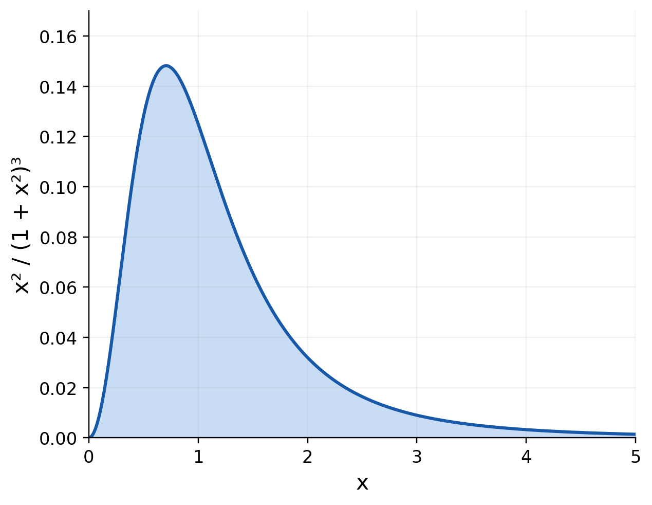
∫[0,∞] x^(a−1)/(1+xᶜ)ᵇ dx = (1/c)B(a/c,b−a/c).
Near zero, convergence needs a>0. At infinity the power is a−1−cb, so convergence needs a<cb.

Deriving the General Form
First set u=xᶜ. Then x^(a−1)dx becomes u^(a/c−1)du/c. The denominator becomes (1+u)ᵇ.
Comparing with the half-line Beta formula gives p=a/c and q=b−a/c. The two inequalities p>0 and q>0 become precisely a>0 and a<cb. The parameter conditions emerge from the substitution rather than being extra rules.
Worked Example 2.92 – A Cubic Denominator
I = ∫[0,∞] x²/(1+x)⁵ dx.
Match p=3 and p+q=5, giving q=2.
I = B(3,2) = (2!1!)/4! = 1/12.
Worked Example 2.93 – A Quadratic Denominator
I = ∫[0,∞] x²/(1+x²)³ dx.
Use a=3,c=2,b=3. Both Beta arguments are 3/2:
I = (1/2)B(3/2,3/2) = π/16.
Worked Example 2.94 – Recognise Divergence
The integral of x²/(1+x²) from 0 to infinity does not converge: the integrand tends to 1. The condition a<cb fails because a=3 while cb=2.
Do not insert such parameters into the convergent Beta integral formula. A formal special-function expression cannot override a failed convergence test.
Recognition Trick
Compare the numerator’s power plus one with the denominator’s effective power at infinity. Write both inequalities before evaluating an improper integral.
36. Dirichlet’s Integral on a Triangle
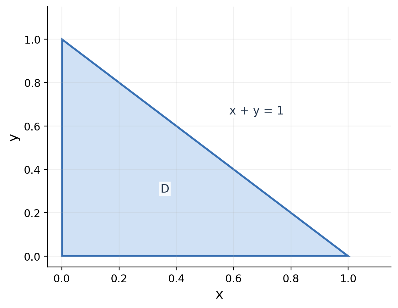
For p,q>0, over D={x≥0,y≥0,x+y≤1}:
∬_D x^(p−1)y^(q−1) dA = Γ(p)Γ(q)/Γ(p+q+1).
The extra +1 in the denominator reflects integration over a filled triangle rather than over the line x+y=1.
Derivation by Direct Integration
First integrate y from 0 to 1−x:
I = (1/q)∫[0,1] x^(p−1)(1−x)ᑫ dx.
I = (1/q)B(p,q+1).
Using Γ(q+1)=qΓ(q) gives the displayed formula.

Worked Example 2.95 – Integrate x²y
Here p=3,q=2:
I = Γ(3)Γ(2)/Γ(6) = (2!1!)/5! = 1/60.
Directly, the y-integration gives x²(1−x)²/2, whose integral is also 1/60.
Worked Example 2.96 – Area as a Special Case
Set p=q=1:
A = Γ(1)²/Γ(3) = 1/2.
This reproduces the area of the unit right triangle.
Worked Example 2.97 – Fractional Endpoint Powers
∬_D dA/√(xy) = Γ(1/2)²/Γ(2) = π.
The integrand is unbounded along the coordinate edges, but both exponents satisfy p,q>0. The improper integral is finite.
Naming Note
Here Dirichlet’s integral refers to simplex integrals used with Beta and Gamma functions. It is not the unrelated one-variable sine-over-x integral that also carries Dirichlet’s name.
37. Dirichlet’s Integral in Space
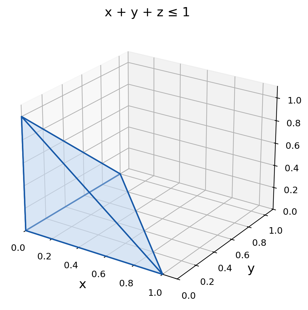
For p,q,r>0 on the unit tetrahedron E={x,y,z≥0,x+y+z≤1}:
∭_E x^(p−1)y^(q−1)z^(r−1) dV = Γ(p)Γ(q)Γ(r)/Γ(p+q+r+1).
Integrating z first produces (1−x−y)ʳ/r. The remaining two-dimensional simplex integral reduces to Beta functions and yields this result.

Worked Example 2.98 – Volume Check
For p=q=r=1:
V = 1/Γ(4) = 1/6.
This agrees with the direct tetrahedron calculation.
Worked Example 2.99 – Integrate xyz
Use p=q=r=2:
I = Γ(2)³/Γ(7) = 1/720.
A common wrong answer is 1/120 from using Γ(6) instead of Γ(7). Check the +1 for the filled simplex.
Worked Example 2.100 – Integrate x²
Here p=3,q=r=1:
I = Γ(3)Γ(1)²/Γ(6) = 1/60.
Dividing by volume 1/6 gives the uniform mean x² as 1/10.
Symmetry Check
The x², y² and z² integrals are identical. Therefore:
∭_E (x²+y²+z²) dV = 1/20.
Boundary Versus Interior
The formula integrates the entire tetrahedral interior, not just its triangular boundary face. A surface integral over x+y+z=1 uses a different measure and is not computed by copying this volume formula.
Exponent Rule
A numerator xᵃyᵇzᶜ corresponds to parameters a+1,b+1,c+1. Convert every exponent before adding the denominator arguments.
38. Scaling a Simplex
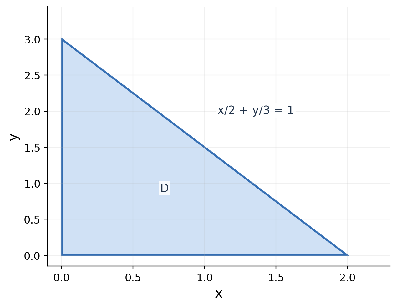
For a,b>0 and p,q>0, the triangle x/a+y/b≤1 in the first quadrant satisfies:
∬_D x^(p−1)y^(q−1) dA = aᵖbᑫ Γ(p)Γ(q)/Γ(p+q+1).
Use x=au, y=bv. The powers contribute a^(p−1)b^(q−1) and the Jacobian contributes ab.

Worked Example 2.101 – Area
With a=2,b=3,p=q=1:
A = ab/2 = 3.
Scaling the Boundary Correctly
Under x=au and y=bv, the sloping edge x/a+y/b=1 becomes u+v=1. The region’s interior maps to u+v≤1.
The same change does not map a rectangle to this triangle. The transformed domain is the unit simplex, so its integral must still use simplex bounds. Scaling simplifies lengths; it does not remove the sloping constraint.
Worked Example 2.102 – Integrate xy
For x/2+y/3≤1:
I = 2²3²Γ(2)²/Γ(5) = 36/24 = 3/2.
Notice that the scale factor is a²b², not merely ab, because the integrand also changes.
Worked Example 2.103 – Scaled Tetrahedron
Let x/2+y/3+z/4≤1 in the first octant. With x=2u,y=3v,z=4w, the volume factor is 24.
V = (2×3×4)/6 = 4.
For integrand xyz, the variable powers contribute another factor 24:
∭_E xyz dV = 24²/720 = 4/5.
General Three-Dimensional Scaling
Replace a,b,c for 2,3,4. The weighted integral has factor aᵖbᑫcʳ multiplying the unit-simplex Gamma ratio.
Dimensional Check
For xyz dV with all coordinates measured in length, the result has units length⁶. The factor a²b²c² has exactly those units.
39. The Full Dirichlet Formula
The leftover fraction can also carry a power. For p,q,r>0 on the unit triangle:
∬_D x^(p−1)y^(q−1)(1−x−y)^(r−1) dA = Γ(p)Γ(q)Γ(r)/Γ(p+q+r).
Setting r=1 gives the earlier filled-triangle formula because Γ(1)=1 and p+q+r=p+q+1.
Worked Example 2.104 – Include the Leftover Factor
I = ∬_D xy(1−x−y) dA.
All three parameters equal 2, hence:
I = Γ(2)³/Γ(6) = 1/120.
This is different from the tetrahedral integral of xyz, whose denominator was Γ(7). The dimensions of the domain differ.
Worked Example 2.105 – A Squared Leftover Fraction
On the unit triangle, integrate (1−x−y)². Choose p=q=1 and r=3:
I = Γ(1)²Γ(3)/Γ(5) = 1/12.
The average of the leftover fraction squared is I/(1/2)=1/6. This result also equals the x² and y² area averages by the symmetry among the three barycentric fractions.
Integrands Depending on x+y
For p,q>0, provided the weighted integral converges, a useful form is:
∬_D x^(p−1)y^(q−1)F(x+y) dA = B(p,q)∫[0,1] s^(p+q−1)F(s) ds.
Use x=st, y=s(1−t), with 0<s<1, 0<t<1 and Jacobian s. The t-integral gives B(p,q).
Worked Example 2.106 – Exponential of the Sum
For p=q=1 and F(s)=eˢ:
∬_D e^(x+y) dA = ∫[0,1] seˢ ds.
I = [(s−1)eˢ] evaluated from s=0 to s=1 = 1.
Worked Example 2.107 – A Power of the Sum
For p=q=1 and F(s)=s²:
∬_D (x+y)² dA = ∫[0,1] s³ ds = 1/4.
Expanding x²+2xy+y² yields 1/12+2/24+1/12=1/4, providing an independent check.
Choose the Form
Use the full simplex formula for powers of x, y and the leftover fraction. Use the sum form when the remaining function depends only on x+y.
When the Sum Form Needs a Limit
If F(s) has a singularity at s=0 or s=1, the remaining one-dimensional integral must be treated as improper. The Beta factor alone does not guarantee convergence for an arbitrary F.
For example, with p=q=1 and F(s)=s^(−2), the remaining integral is ∫[0,1] s^(−1) ds and diverges. The singularity near the triangle’s origin is too strong.
40. Image Processing: Intensity Sums
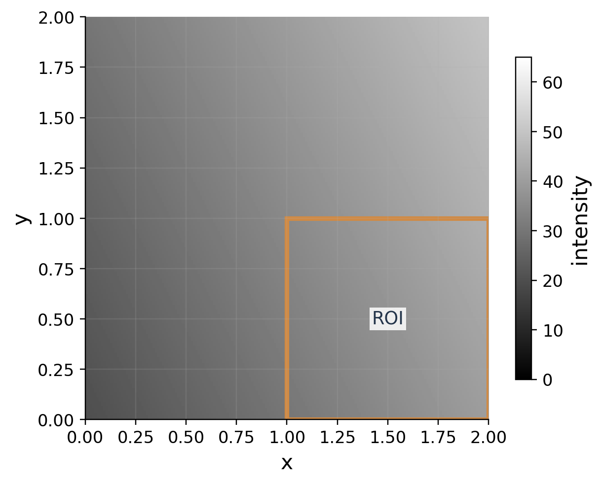
A grayscale image can be modelled by an intensity field I(x,y) over a rectangular region. A double integral gives total intensity; dividing by area gives average intensity.
Real digital images consist of pixels. With unit-area pixels, summation is exact for a piecewise-constant pixel model. For a smooth field sampled at pixel centres, the weighted sum is a numerical approximation.

Region of Interest
For a selected region R:
T_R = ∬_R I(x,y) dA, Ī_R = T_R/A_R.
If pixels are not unit area, their area weights must remain in the sum.
Pixel Coordinates and Area Weights
If an image occupies a physical rectangle of width W and height H with nₓ columns and nᵧ rows, an equal pixel cell has area WH/(nₓnᵧ).
A total-intensity approximation multiplies every sampled intensity by this cell area. An average divides the total by WH, so the common area factor cancels and leaves the ordinary arithmetic mean of equal-area pixel values.
Worked Example 2.108 – Mean Grayscale Level
Let I(x,y)=20+10x+5y over 0≤x≤2, 0≤y≤2. The field ranges from 20 to 50, within an 8-bit grayscale range.
T = ∫[0,2] ∫[0,2] (20+10x+5y) dy dx.
The y-integration gives 50+20x. The remaining integral gives T=140. Since the area is 4:
Ī = 35.
Worked Example 2.109 – A Smaller Image Region
Restrict to 1≤x≤2, 0≤y≤1. Its area is 1 and its average coordinates are 3/2 and 1/2.
Ī_R = 20+10(3/2)+5(1/2) = 75/2.
Thus T_R=37.5. The smaller region has a larger mean intensity but a smaller total intensity than the full image.
Interpretation
Total brightness depends on both intensity and area. Comparing totals from differently sized regions does not by itself compare their average brightness.

41. Intensity-Weighted Image Centres
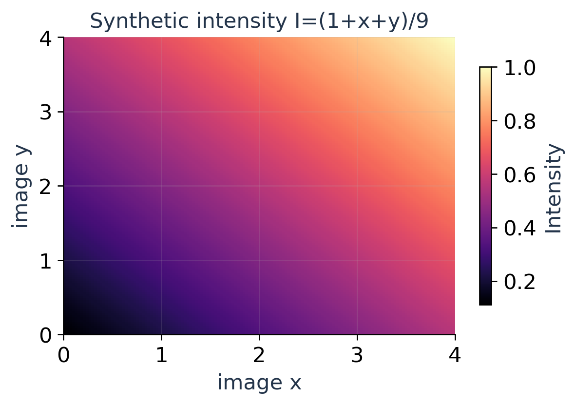
For a nonnegative intensity field with total T>0, an intensity-weighted centre is:
x̄ = (∬_D xI(x,y) dA)/T, ȳ = (∬_D yI(x,y) dA)/T.
This mathematical construction is useful for understanding image moments and bright-object localisation. A practical algorithm may also require background subtraction, thresholding or noise handling.

Worked Example 2.110 – Total Intensity
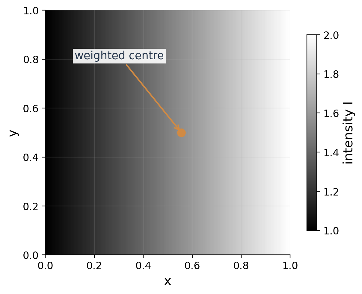
For I=1+x on the unit square:
T = ∫[0,1] ∫[0,1] (1+x) dy dx = 3/2.
Compute the Weighted Centre
The x-coordinate moment is:
M_y = ∫[0,1] x(1+x) dx = 1/2+1/3 = 5/6.
The y-coordinate moment is:
M_x = (∫[0,1] (1+x) dx)(∫[0,1] y dy) = 3/4.
Therefore:
x̄ = (5/6)/(3/2) = 5/9, ȳ = (3/4)/(3/2) = 1/2.
The x-coordinate moves right from the geometric centre 1/2. The y-coordinate stays 1/2 because the intensity does not change with y.
Worked Example 2.111 – Discrete Pixel Check
Take two equal-area columns with centre positions x=1/4 and 3/4, and intensities 5/4 and 7/4. Their discrete weighted centre is:
x̄_disc = [(1/4)(5/4)+(3/4)(7/4)]/[5/4+7/4] = 13/24.
This differs from the continuous value 5/9 because the coarse pixel-centre approximation does not exactly integrate the quadratic moment x(1+x).
Practical Check
A centre computed with nonnegative weights must lie inside the convex hull of the weighted pixel locations. A result outside the image usually indicates incorrect normalisation or signed weights.
42. Data Density and Normalisation
A spatial count density λ(x,y) gives expected count per unit area. Integrating λ over a region gives an expected count, which need not equal one.
A probability density f(x,y) instead satisfies f≥0 and total integral one. A count density can be normalised to describe the location of a randomly selected item when its total count is finite and positive.

Worked Example 2.112 – Expected Counts
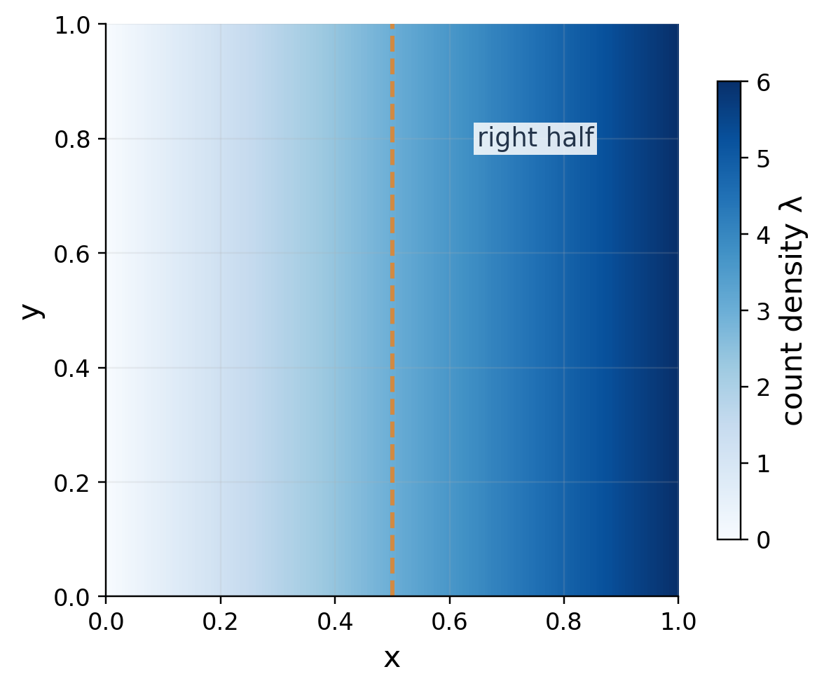
Let λ=6x on the unit square. Then:
N = ∫[0,1] ∫[0,1] 6x dy dx = 3.
In the right half, 1/2≤x≤1, the expected count is:
N_R = ∫[1/2,1] 6x dx = 9/4.
Normalising the Same Field
The corresponding location density is f=λ/N=2x on the unit square and zero elsewhere. Its integral is one.
Worked Example 2.113 – Right-Half Probability
P(X≥1/2) = ∫[1/2,1] ∫[0,1] 2x dy dx = 3/4.
The probability 3/4 equals the fraction of expected count in that half: (9/4)/3.
A Histogram Estimate
Suppose a two-dimensional data histogram has N observations and a cell of area ΔA contains n observations. A piecewise-constant density estimate in that cell is n/(NΔA).
Its integrated probability contribution is n/N. Summing over all cells gives one when all observations are assigned exactly once.
Worked Example 2.114 – One Cell
For N=100, n=12 and ΔA=0.04, the density estimate is 3. The cell’s probability is 3×0.04=0.12.
A density value larger than one is valid; it is probability per unit area. The integrated probability of any event cannot exceed one.
Distinguish Quantities
Expected count, probability density and event probability have different meanings. State which one the integrand represents before interpreting the integral.
43. Joint Probability Distributions
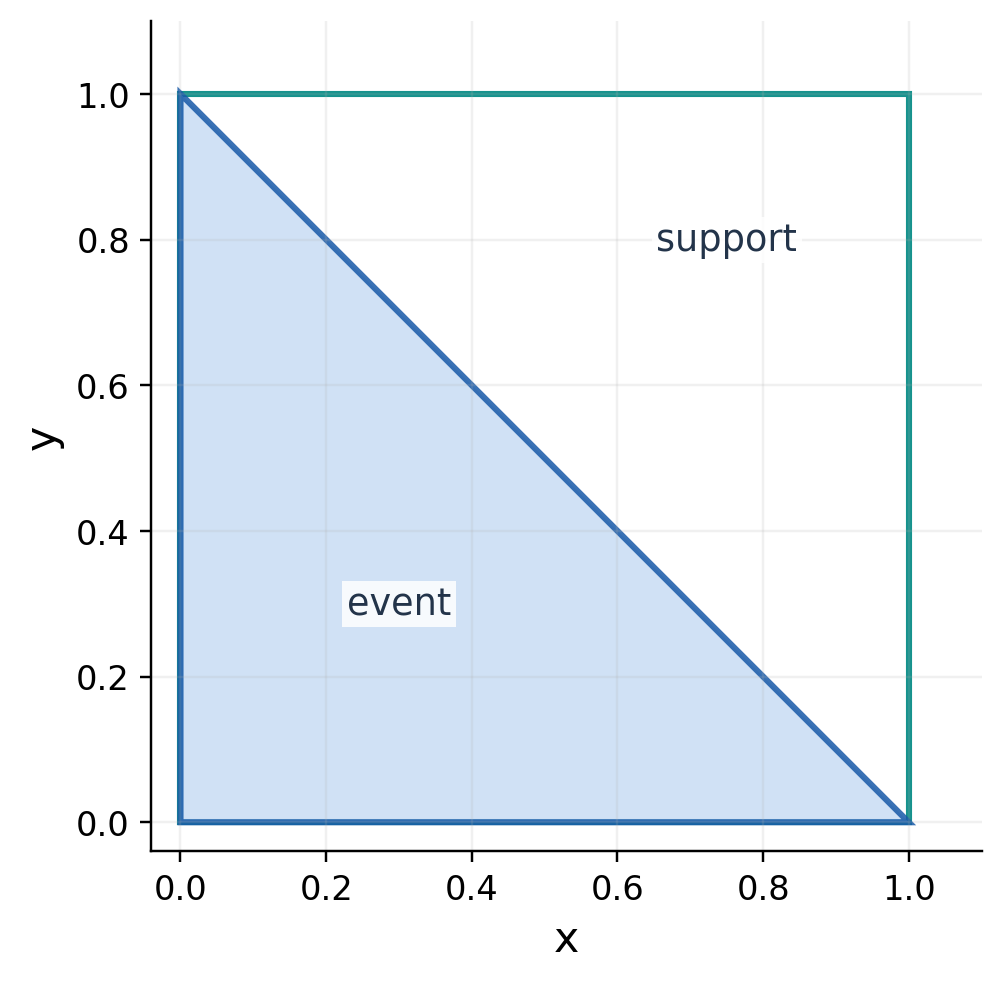
For continuous random variables X,Y, a joint density f must be nonnegative and integrate to one over its support. An event probability is an integral over the event intersected with that support.
Worked Example 2.115 – Find a Normalising Constant
Let f(x,y)=c(x+y) on the unit square and zero elsewhere.
1 = c∫[0,1] ∫[0,1] (x+y) dy dx = c.
Thus c=1. The density is nonnegative on its stated support.

Worked Example 2.116 – Probability Below a Line
Using f=x+y:
P(X+Y≤1) = ∫[0,1] ∫[0,1−x] (x+y) dy dx.
The inner integral simplifies to (1−x²)/2. Therefore:
P = (1/2)∫[0,1] (1−x²) dx = 1/3.
The triangle has area 1/2, but its probability is 1/3 because the density is not uniform and is smaller near the origin.
Worked Example 2.117 – Right-Half Probability
P(X>1/2) = ∫[1/2,1] (x+1/2) dx = 5/8.
Equality or strict inequality at a line makes no difference for a continuous density: a single line has zero two-dimensional area.
Support Matters
For an event extending outside [0,1]², integrate only the overlap with the support. The density is zero elsewhere. A diagram of the overlap is often the quickest way to choose correct limits.
Probability Check
Every event probability must be between 0 and 1. Area equals probability only for a suitably normalised uniform distribution, not for every density.
44. Marginals and Independence
The marginal density of X integrates out Y:
f_X(x) = ∫[−∞,∞] f(x,y) dy.
Similarly, f_Y(y) integrates out x. Bounds can be restricted to the support, but any support dependence must remain in the limits.
Worked Example 2.118 – Marginals on a Square
For f=x+y on [0,1]²:
f_X(x) = x+1/2, 0≤x≤1.
f_Y(y) = y+1/2, 0≤y≤1.
Each integrates to one. Outside its interval, each marginal is zero.
Independence Test
X and Y are independent when the joint density equals the product of its two marginals almost everywhere. Here the product (x+1/2)(y+1/2) is not x+y, so they are not independent.
Worked Example 2.119 – A Marginal on a Triangle
For the uniform triangular density f=2 on x,y≥0,x+y≤1:
f_X(x) = ∫[0,1−x] 2 dy = 2(1−x).
It is zero outside 0≤x≤1. Its integral is 1. The changing upper bound records the shrinking vertical slice and explains why the marginal is not uniform even though the joint density is constant inside the triangle.
Worked Example 2.120 – A Product Density
Let f=4xy on the unit square and zero elsewhere. It integrates to one because:
∫[0,1] ∫[0,1] 4xy dy dx = 1.
The marginals are f_X=2x and f_Y=2y, whose product is exactly 4xy. Hence these variables are independent.
Worked Example 2.121 – A Rectangular Event
P(X≤1/2,Y≤1/2) = (∫[0,1/2] 2x dx)(∫[0,1/2] 2y dy) = 1/16.
A Triangular Support Warning
Even a constant joint density on the triangle x≥0,y≥0,x+y≤1 does not make X and Y independent. The support itself couples them: a large x forces y to be small.
For its uniform density f=2, the marginal is f_X(x)=2(1−x), not a constant.
Independence Habit
Check both the formula and the support. A factorable expression inside a nonrectangular support is not enough to establish independence.
Worked Example 2.122 – A Conditional Probability
For the independent product density 4xy on the unit square, P(X≤1/2)=1/4 and P(Y≤1/2)=1/4.
Thus P(X≤1/2 given Y≤1/2) equals (1/16)/(1/4)=1/4. Conditioning on that Y-event does not change the X-probability. This checks independence using an event calculation as well as the density factorisation.
45. Expectations and Covariance
For an integrable function g(X,Y):
E[g(X,Y)] = ∬ g(x,y)f(x,y) dA.
Use g=x for E[X], g=y for E[Y], and g=xy for E[XY]. The covariance is:
Cov(X,Y) = E[XY]−E[X]E[Y].
These are density-weighted averages. The extra x, y or xy factor must appear in the integrand.
Worked Example 2.123 – Uniform Unit Triangle
Let f=2 on x,y≥0,x+y≤1. Then:
E[X] = 2∬_D x dA = 1/3.
By symmetry E[Y]=1/3. The result also matches the geometric centroid of the triangle.
Computing a Mean Needs Normalisation
For the triangular support, the integral of x alone is 1/6. The density is 2, so the expectation is 2×1/6=1/3.
The raw geometric moment and the probability expectation are related but not interchangeable. With a nonuniform density, every point receives its own density weight instead of one common factor.
Compute Second Moments
For the same distribution:
E[X²] = 2(1/12) = 1/6.
E[XY] = 2(1/24) = 1/12.
Thus:
Var(X) = 1/6−1/9 = 1/18.
Cov(X,Y) = 1/12−1/9 = −1/36.
The negative covariance agrees with the support: if one coordinate is large, the other has less room to grow.
Worked Example 2.124 – A Linear Combination
E[X+2Y] = E[X]+2E[Y] = 1.
Linearity of expectation does not require independence. However, replacing E[XY] by E[X]E[Y] would be invalid here.
AI Interpretation
A probabilistic model can use expectations to describe average feature values and covariance to describe linear association. The calculations above concern the stated synthetic distribution; they do not imply a fitted model or real dataset.
Moment Check
Variance must be nonnegative. Covariance may be positive, negative or zero. Zero covariance alone does not generally prove independence.
Worked Example 2.125 – Variance of the Sum
Use the covariance identity:
Var(X+Y) = Var(X)+Var(Y)+2Cov(X,Y).
Var(X+Y) = 1/18+1/18−2/36 = 1/18.
A direct check uses E[(X+Y)²]=1/2 and E[X+Y]=2/3, giving 1/2−4/9=1/18. Negative covariance reduces the variance of the sum compared with treating the coordinates as independent.
46. Gaussian Probability in Two Dimensions
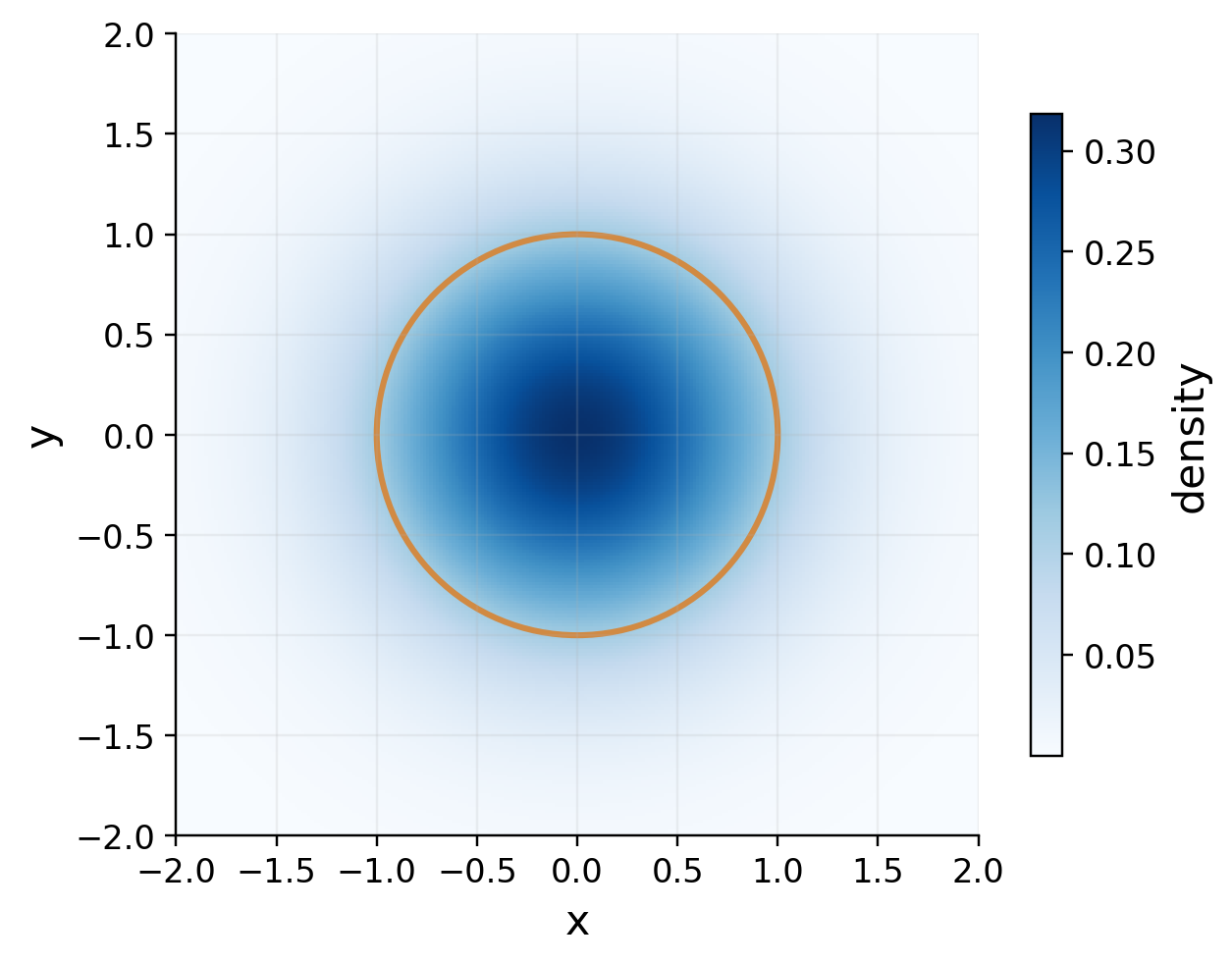
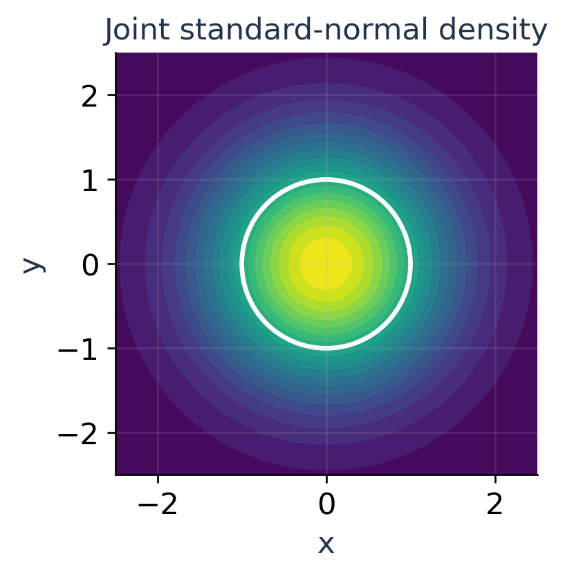
Consider the normalised radial density:
f(x,y) = (1/π)e^(−(x²+y²)), (x,y)∈ℝ².
Its full-plane integral is one because the unnormalised Gaussian integral is π. In polar coordinates, event probabilities become simple radial integrals.

Worked Example 2.126 – Probability Within Radius a
For a≥0:
P(X²+Y²≤a²) = (1/π)∫[0,2π] ∫[0,a] e^(−r²)r dr dθ.
P = 1−e^(−a²).
At a=1 this is approximately 0.6321.
Worked Example 2.127 – An Annulus
For 1≤r≤2:
P(1≤R≤2) = e^(−1)−e^(−4).
Subtract the cumulative probabilities or integrate directly. The result is positive and smaller than the probability outside r=1, which is e^(−1).
Worked Example 2.128 – Mean Squared Radius
E[R²] = 2∫[0,∞] r³e^(−r²) dr.
Set t=r², so r³dr=t dt/2:
E[R²] = ∫[0,∞] te^(−t) dt = Γ(2) = 1.
Symmetry gives E[X²]=E[Y²]=1/2. Both coordinate means are zero, so each variance is 1/2.
General Isotropic Gaussian
For σ>0, the density is (2πσ²)^(−1)exp[−r²/(2σ²)]. Its disk probability is:
P(R≤a) = 1−e^(−a²/(2σ²)).
Do not mix this variance convention with e^(−r²)/π. The latter corresponds to σ²=1/2.
Radial Probability
Probability in a ring includes its circumference factor. The radial density is 2r e^(−r²), not e^(−r²)/π.

47. Beta and Dirichlet Probability Models
A Beta density on 0<t<1 has positive parameters p,q:
f(t) = t^(p−1)(1−t)^(q−1)/B(p,q).
It is normalised by the Beta integral. The mean follows by shifting the first argument:
E[T] = B(p+1,q)/B(p,q) = p/(p+q).
Worked Example 2.129 – Beta(2,3)
Since B(2,3)=1/12:
f(t) = 12t(1−t)², E[T] = 2/5.
For T≤1/2, expand t−2t²+t³ and integrate:
P(T≤1/2) = 12[t²/2−2t³/3+t⁴/4] evaluated from t=0 to t=1/2 = 11/16.
Probabilities for Three Proportions
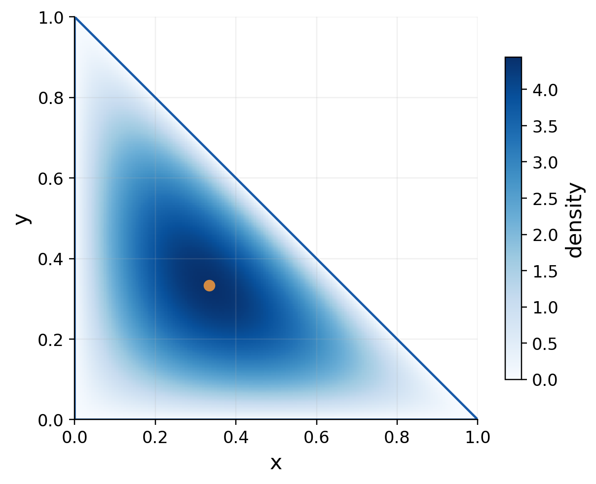
A Dirichlet model describes nonnegative proportions x,y,z with x+y+z=1. Two coordinates are free and z=1−x−y.
For positive α,β,γ, the density with respect to dx dy on the unit triangle is:
f(x,y) = {Γ(α+β+γ)/[Γ(α)Γ(β)Γ(γ)]} × x^(α−1)y^(β−1)(1−x−y)^(γ−1).
Worked Example 2.130 – Three Equal Parameters
For α=β=γ=2, the normalising constant is Γ(6)/Γ(2)³=120.
f(x,y) = 120xy(1−x−y).
The full Dirichlet integral is 1/120, so the density integrates to one. Symmetry and x+y+z=1 give E[X]=E[Y]=E[Z]=1/3.

Measure Matters
This density is expressed using the two free coordinates dx dy. It is not an ordinary three-dimensional volume density on a solid tetrahedron.
Why This Model Suits Proportions
Three proportions must add to one. Raising x while fixing y forces z=1−x−y to decrease, so the coordinates cannot vary independently.
The Dirichlet density builds this constraint into its support. In the symmetric (2,2,2) example, permutations of the three proportions preserve the distribution, which explains the equal means without an additional long moment calculation.


48. Mixed Solved Revision: Geometry
Worked Example 2.131 – Reverse a Curved Order
Evaluate:
I = ∫[0,1] ∫[y,1] x² dx dy.
The inequalities are 0≤y≤x≤1. Reversing gives:
I = ∫[0,1] ∫[0,x] x² dy dx.
I = ∫[0,1] x³ dx = 1/4.
Directly the original order gives ∫[0,1] (1−y³)/3 dy=1/4, confirming the result.
Worked Example 2.132 – Area by Order Reversal
For D={0≤x≤1,x²≤y≤x}, use horizontal slices:
A = ∫[0,1] (√y−y) dy = 1/6.
This checks the curved region’s two descriptions without carrying a complicated integrand.
Worked Example 2.133 – A Disk Polynomial
Evaluate (x²+y²)² over the unit disk. The integrand becomes r⁴ and the element contributes r:
I = ∫[0,2π] ∫[0,1] r⁵ dr dθ = π/3.
The value lies between 0 and the disk area π.
Worked Example 2.134 – An Elliptic Cap
Find the volume under z=1−x²/4−y²/9 and above z=0. Use x=2r cos θ, y=3r sin θ, with 0≤r≤1 and a full turn.
|J| = 6r.
V = 6∫[0,2π] ∫[0,1] (1−r²)r dr dθ = 3π.
The base ellipse has area 6π and maximum height 1. The average height is 1/2, so 3π is consistent.
Worked Example 2.135 – A Scaled Tetrahedron
For x+y+z≤2 in the first octant, scaling all coordinates by 2 multiplies volume by 8:
V = 2³/6 = 4/3.
Revision Strategy
Identify the geometric type before integrating. A correct region and coordinate choice usually remove more work than an advanced antiderivative trick.
A Volume Scale Check
If every linear dimension of a solid is multiplied by c>0, volume scales by c³. A first coordinate moment scales by c⁴ because the integrand contributes one more length factor.
For the radius-a ball, the integral of squared radius scales by a⁵: three powers from volume and two from the integrand. These checks are useful before expanding any antiderivative.
49. Mixed Solved Revision: Special Functions
Worked Example 2.136 – An Exponential Moment
I = ∫[0,∞] x³e^(−2x) dx.
Here m=4,k=1,a=2:
I = 2^(−4)Γ(4) = 6/16 = 3/8.
Worked Example 2.137 – A Beta Integral on [0,2]
I = ∫[0,2] x^(1/2)(2−x)^(1/2) dx.
Set p=q=3/2 and a=2. The interval-scaling factor is 2^(p+q−1)=4:
I = 4B(3/2,3/2) = π/2.
Geometrically the integrand is √[1−(x−1)²], the upper semicircle of radius one. Its area is π/2, independently confirming the result.
Worked Example 2.138 – A Scaled Gaussian Moment
I = ∫[0,∞] xe^(−5x²) dx.
Set t=5x², so x dx=dt/10:
I = (1/10)∫[0,∞] e^(−t) dt = 1/10.
This is the general Gamma formula with m=2,k=2,a=5. Both methods give the same exact result without needing a Gaussian square-root constant.
Worked Example 2.139 – A Weighted Triangle
Over x,y≥0,x+y≤1, evaluate x²y².
I = Γ(3)²/Γ(7) = 4/720 = 1/180.
The denominator argument is p+q+1=7. The numerator arguments are both 3.
Worked Example 2.140 – A Leftover Power
Evaluate x(1−x−y)² over the same triangle. Parameters are p=2,q=1,r=3:
I = Γ(2)Γ(1)Γ(3)/Γ(6) = 1/60.
Worked Example 2.141 – A Scaled Spatial Moment
Over x/2+y/3+z≤1 in the first octant, evaluate x. Use p=2,q=r=1 and scales a=2,b=3,c=1:
I = 2² × 3 × Γ(2)Γ(1)²/Γ(5) = 1/2.
The tetrahedron has volume 1 and centroid x=2/4=1/2, giving the same moment.
Independent Checks
A geometric interpretation, symmetry calculation or scale test can reveal a wrong factorial even when the algebra looks orderly.
Worked Example 2.142 – Uniform Tetrahedron Mean
The unit tetrahedron has volume 1/6 and x-moment 1/24. Its uniform probability density is therefore 6, not 1.
E[X] = 6∭_E x dV = 1/4.
By symmetry all three coordinate means equal 1/4. The remaining mean fraction 1−X−Y−Z is also 1/4, matching the four symmetric simplex coordinates.
50. Common Errors, Corrected
Error: Swap Differentials Only
Wrong: reverse a triangular integral but retain the old numerical and functional limits.
Correct: rewrite the region as inequalities, project on the new outer axis, and solve the boundaries for the new inner variable.
Error: Forget the Polar Factor
Wrong: integrate a disk using dr dθ alone.
Correct: dA=r dr dθ. For a unit disk, the correct integral of one is π; the missing-factor calculation produces 2π.
Error: Use a Signed Area Factor
Wrong: retain J=−1/2 as the measure in a planar substitution.
Correct: use |J|=1/2. Orientation does not make area or a positive density integral negative.
Error: Treat a Triangle as a Rectangle
Wrong: factor ∬xy into independent x and y integrals when y≤1−x.
Correct: keep the coupled bound or use a justified simplex formula.
Error: Misread a Gamma Power
Wrong: x⁴e^(−x) gives Γ(4).
Correct: exponent s−1=4 gives Γ(5)=24.
Error: Drop the Dirichlet +1
Wrong: on the filled triangle, use Γ(p+q) in the denominator for x^(p−1)y^(q−1).
Correct: use Γ(p+q+1). The p=q=1 area check must give 1/2.
Error: Ignore Convergence
Wrong: apply a Beta identity to an integral whose tail tends to a nonzero constant.
Correct: test both endpoints. An improper integral must converge before its finite Beta value can be used.
Error: Confuse Density with Probability
Wrong: reject a density value 3 because it exceeds one.
Correct: density is per unit area; integrate it over the event. A cell of area 0.04 with density 3 has probability 0.12.
Final Audit
Region, bounds, integrand, differential element, convergence, sign, units and expected size should agree. These checks catch different mistakes and are most useful together.
Error: Confuse a Cone with a Cap
Wrong: describe z≥a/2 inside a sphere by the constant angle φ≤π/4.
Correct: translate the plane as ρ cos φ≥a/2. A horizontal cut couples radius and angle. A cone through the origin gives a constant polar angle; a plane above the origin generally does not.
The boundary type should be identified before borrowing familiar spherical limits.
51. Short-Answer Checks with Answers
What Does dy dx Mean?
Integrate y first while x is fixed. Insert the y-limits; then integrate the resulting x-expression.
When Is a Double Integral a Volume?
When the integrand is a nonnegative vertical height above the stated base region. For two surfaces, use upper minus lower wherever that difference is nonnegative.
Why Does a Polar Integral Contain r?
A small polar cell has sides approximately dr and r dθ. Their product is r dr dθ; equivalently, the absolute Jacobian is r.
Why Can Changing Order Require a Split?
A new family of slices may encounter different boundary curves in different outer-variable intervals. Each interval needs the appropriate entry and exit functions.
Does a Negative Jacobian Give Negative Area?
No. The sign records orientation. Area and volume substitutions use the absolute determinant.
State Γ(n) for a Positive Integer n.
Γ(n) = (n−1)!, so Γ(1)=1 and Γ(5)=24.
State the Beta–Gamma Relation.
For positive real p,q:
B(p,q) = Γ(p)Γ(q)/Γ(p+q).
Can an Unbounded Integrand Have a Finite Integral?
Yes. For example, t^(−1/2) is unbounded near zero but integrable there. Check the power and the endpoint limit rather than the height alone.
Does a Factorable Density Imply Independence?
Only when the full joint density, including its support, equals the product of its marginals almost everywhere. A coupled triangular support can prevent independence.
How Is an Image Mean Different from Total Intensity?
The total integrates intensity over the region. The mean divides that total by the region’s area.
What Does a Marginal Density Do?
It integrates out the other variable over the allowed support, leaving a one-variable density.
Answer-Writing Habit
Give the rule and its condition together. A short complete answer is more useful than a memorised formula without its domain or interpretation.
52. Formula Sheet: Regions and Measures
Cartesian Double Integrals
For a vertically simple region:
∬_D f dA = ∫[a,b] ∫[g₁(x),g₂(x)] f dy dx.
For a horizontally simple region:
∬_D f dA = ∫[c,d] ∫[h₁(y),h₂(y)] f dx dy.
Area and Volume
A = ∬_D 1 dA.
V = ∬_D (upper−lower) dA.
V = ∭_E 1 dV.
Require upper≥lower on D for the geometric volume formula.
General Transformation
dA = |∂(x,y)/∂(u,v)| du dv.
Use a suitable one-to-one coordinate patch and the transformed domain. Split domains when necessary.
Bound-Writing Template
For dz dy dx, write the x-interval first in words, then the y-range at fixed x, then the z-range above each base point. Place them in the integral from outermost to innermost.
The integration is executed in the reverse direction: z first, then y, then x. Distinguishing the writing sequence from the calculation sequence makes nested limits easier to organise.
Polar Coordinates
x = r cos θ, y = r sin θ.
dA = r dr dθ.
Cylindrical Coordinates
x = r cos θ, y = r sin θ, z = z.
dV = r dz dr dθ.
Spherical Coordinates
Here φ is measured from +z:
x = ρ sin φ cos θ, y = ρ sin φ sin θ.
z = ρ cos φ.
dV = ρ² sin φ dρ dφ dθ.
Means and Moments
f_avg = (1/A)∬_D f dA.
M = ∬_D ρ dA.
x̄ = (1/M)∬_D xρ dA, ȳ = (1/M)∬_D yρ dA.
Averages divide by area; density-weighted centres divide by mass or total weight. Identify the intended denominator before substitution.
Standard Angular Intervals
A full turn uses 0≤θ≤2π. An upper half-ball uses 0≤φ≤π/2 and the full θ-range. A first-octant ball uses both angles from 0 to π/2.
These intervals use the stated spherical convention. They should be derived from coordinate signs whenever a diagram or a textbook uses a different angle convention.
53. Formula Sheet: Special Integrals
For s,p,q>0:
Γ(s) = ∫[0,∞] t^(s−1)e^(−t) dt.
Γ(s+1) = sΓ(s), Γ(1/2) = √π.
B(p,q) = ∫[0,1] t^(p−1)(1−t)^(q−1) dt.
B(p,q) = Γ(p)Γ(q)/Γ(p+q) = B(q,p).
For a,k,m>0:
∫[0,∞] x^(m−1)e^(−axᵏ) dx = (1/k)a^(−m/k)Γ(m/k).
For m,n>−1:
∫[0,π/2] sinᵐt cosⁿt dt = (1/2)B((m+1)/2,(n+1)/2).
For c>0 and 0<a<cb:
∫[0,∞] x^(a−1)/(1+xᶜ)ᵇ dx = (1/c)B(a/c,b−a/c).
Conditions Belong with Formulas
Integer factorial rules apply to positive integer Gamma arguments. Half-integer values reduce through Γ(1/2)=√π. General positive noninteger arguments may remain as Gamma values.
For a rational half-line Beta integral, the lower and upper endpoint conditions are separate. If either fails, use a divergence argument rather than reporting a finite formula outside its permitted range.
Dirichlet Formulas
For positive p,q on x,y≥0,x+y≤1:
∬_D x^(p−1)y^(q−1) dA = Γ(p)Γ(q)/Γ(p+q+1).
For positive p,q,r on the same triangle:
∬_D x^(p−1)y^(q−1)(1−x−y)^(r−1) dA = Γ(p)Γ(q)Γ(r)/Γ(p+q+r).
For positive p,q,r on the unit tetrahedron:
∭_E x^(p−1)y^(q−1)z^(r−1) dV = Γ(p)Γ(q)Γ(r)/Γ(p+q+r+1).
Final Self-Checks with Results
- Unit-disk area: π; unit-ball volume: 4π/3.
- Integral of x²+y² over the unit disk: π/2.
- Γ(5): 24; Γ(5/2): 3√π/4.
- B(2,3): 1/12; B(1/2,1/2): π.
- Integral of xy over the unit triangle: 1/24.
- Integral of xyz over the unit tetrahedron: 1/720.
Complete Solution Standard
State the region and assumptions, show the useful substitution or order, evaluate the limits clearly, and interpret the final value with a sign, units or probability check.


