
University: Dr. A.P.J. Abdul Kalam Technical University (AKTU) Programme: B.Tech First Year, Semester I & II Course Codes: AAS102D / AAS202D Stream: CSE Unit: IV
Introduction
Nanomaterials and Functional Materials for Smart Systems connects nanoscale structure with electrical, optical, surface and mechanical responses. Learn how the material works, where it is useful and what limits a real device.
Syllabus Coverage
Nanotechnology; carbon nanotubes; graphene; quantum dots; smart coatings; self-cleaning and hydrophobic surfaces; photochromic and thermochromic materials; shape-memory polymers; flexible electronics and smart devices.
Topic Map
| Topic | PDF Pages |
|---|---|
| Nanoscale effects and preparation | 2–8 |
| Carbon nanotubes and networks | 8–12 |
| Graphene and thin-film electrodes | 12–17 |
| Quantum dots and displays | 17–22 |
| Smart coatings and wetting | 22–27 |
| Self-cleaning mechanisms | 27–30 |
| Photochromic and thermochromic materials | 30–33 |
| Shape-memory polymers | 33–38 |
| Flexible and smart devices | 38–43 |
| Formula guide and complete revision | 43–46 |
How to Study This Unit
- Connect structure with a useful property.
- Separate surface effects from confinement.
- Distinguish a film from a complete device.
- Keep sheet and contact resistance distinct.
- Use photon energy without inventing a size law.
- Separate static wetting from drop mobility.
- Name the self-cleaning mechanism.
- Identify the trigger and recovery conditions.
- Distinguish shape fixity from recovery.
- Convert strain percentages to fractions.
Main Principle: Explain material → mechanism → measured response → application. Include a relevant limitation whenever an ideal property is connected to a real device.
1. Nanotechnology: Scale, Surface and Function
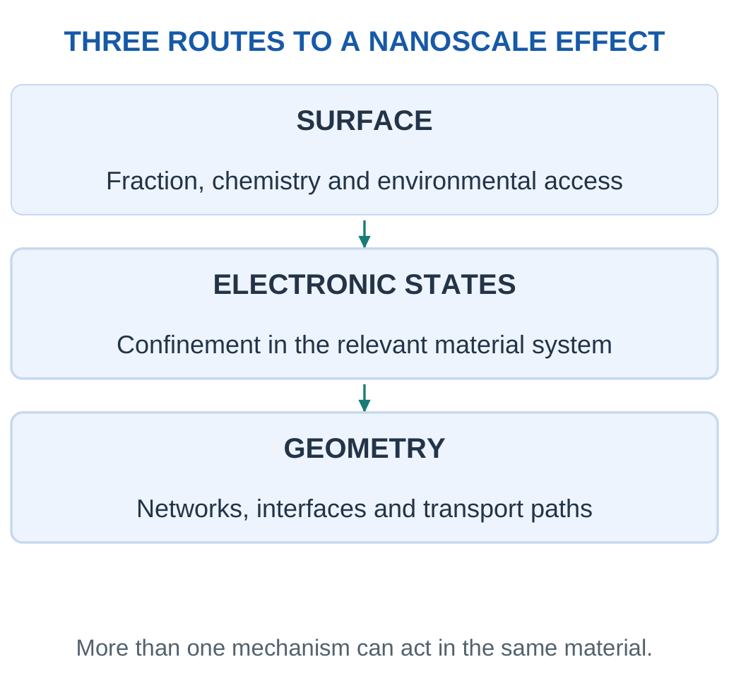
Nanotechnology concerns understanding and engineering matter at roughly 1–100 nm to use behaviour associated with that scale. One nanometre equals 10⁻⁹ m. A nanoscale dimension can change the fraction of material at interfaces, the available electronic states or the way structures connect. These are distinct mechanisms, not one universal nano effect.
Why Size Matters
Atoms at a surface have a different environment from those deep inside a solid. Subdividing a material into smaller, separated particles increases exposed area per unit volume. This can affect adsorption, chemical reaction and interaction with a surrounding polymer. Aggregation can reduce the area actually accessible to a liquid or gas.

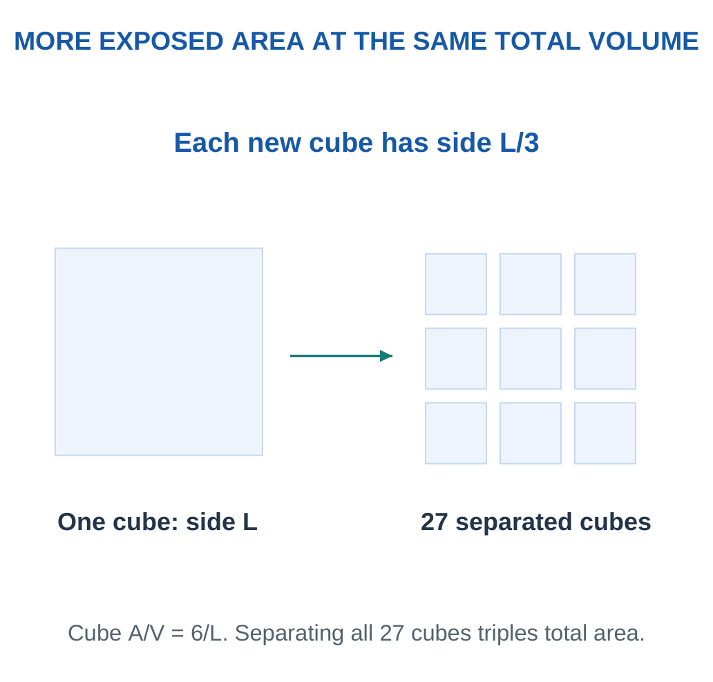
For a sphere of diameter d:
- Surface area, A = πd²
- Volume, V = πd³/6
- A/V = 6/d
For a cube of side L:
A/V = 6/L
Use one consistent length unit. With d in metres, A/V is in m⁻¹.
Key Point: Area Is Not Activity
A larger geometric area can increase opportunities for interaction, but surface chemistry, crystal faces, contamination and access also matter. Deriving A/V does not derive a reaction-rate law. Compare accessible area and functional response separately.
Connect Property to a Device
A sensor needs a responsive interface, a display needs controlled emission and a wearable needs electrical continuity during bending. A nanomaterial can contribute to these requirements, but contacts, support, packaging and processing still determine the complete device. The smallest particle is not automatically the best choice.
Examination Pattern: Define the scale → explain the physical mechanism → name a material → connect a useful property to an application → add one limitation.
Surface Area, Activity and Stability
A larger exposed area can create more opportunities for interaction, but activity per unit area can change with crystal face, surface groups or contamination. A comparison of equal masses should also account for density and shape. Two powders with the same nominal diameter can have different accessible areas if one is porous or strongly aggregated.
A protective organic layer can prevent particles from sticking together while reducing access to a catalytic or sensing surface. Removing the layer may increase access but worsen dispersion or stability. This shows why a processing improvement must be checked against the actual device function.
A Simple Derivation
For N identical spheres:
- Total area = Nπd²
- Total volume = Nπd³/6
Dividing cancels N and gives 6/d.
If total solid volume remains fixed while d is reduced, N must increase. It is the combination of more particles and smaller individual size that increases total area; one smaller sphere by itself has less area than one larger sphere.
From Nanometres to an Engineering Specimen
An electronic film can be centimetres wide and still contain a nanoscale feature. A coating may have nanoscale particles dispersed through a much thicker layer; a wire can be very long while its diameter lies in the nanoscale range. The important question is which dimension controls the proposed behaviour. Calling an entire object nano without identifying that feature leaves the explanation incomplete.
One micrometre contains 1000 nm, while one millimetre contains one million nm. A 50 nm particle is therefore 0.05 μm, not 50 μm. A specimen made from many such particles can be easily visible even though an individual particle cannot be resolved by ordinary eyesight.
Equal Number, Equal Mass and Equal Volume
Comparisons must state what is held constant. One 20 nm sphere has less area than one 100 nm sphere. At equal total volume of solid, however, many more 20 nm spheres are needed and their combined area is larger. Equal mass is equivalent to equal solid volume only when the relevant density is the same.


Area-to-Mass Relation
For smooth spheres with density ρ:
- Mass = ρπd³/6
- Surface area = πd²
- Specific geometric area = 6/(ρd)
With density in kg/m³ and diameter in m, the result is m²/kg. The expression assumes fully exposed surfaces and no internal porosity. A porous or aggregated powder needs a measurement of accessible area rather than treating this estimate as exact.
Concept Connection: Geometry predicts an area opportunity. Surface chemistry and access determine what that opportunity means for adsorption, reaction or sensing.
Application Workshop: Nominal Size Versus Accessible Area
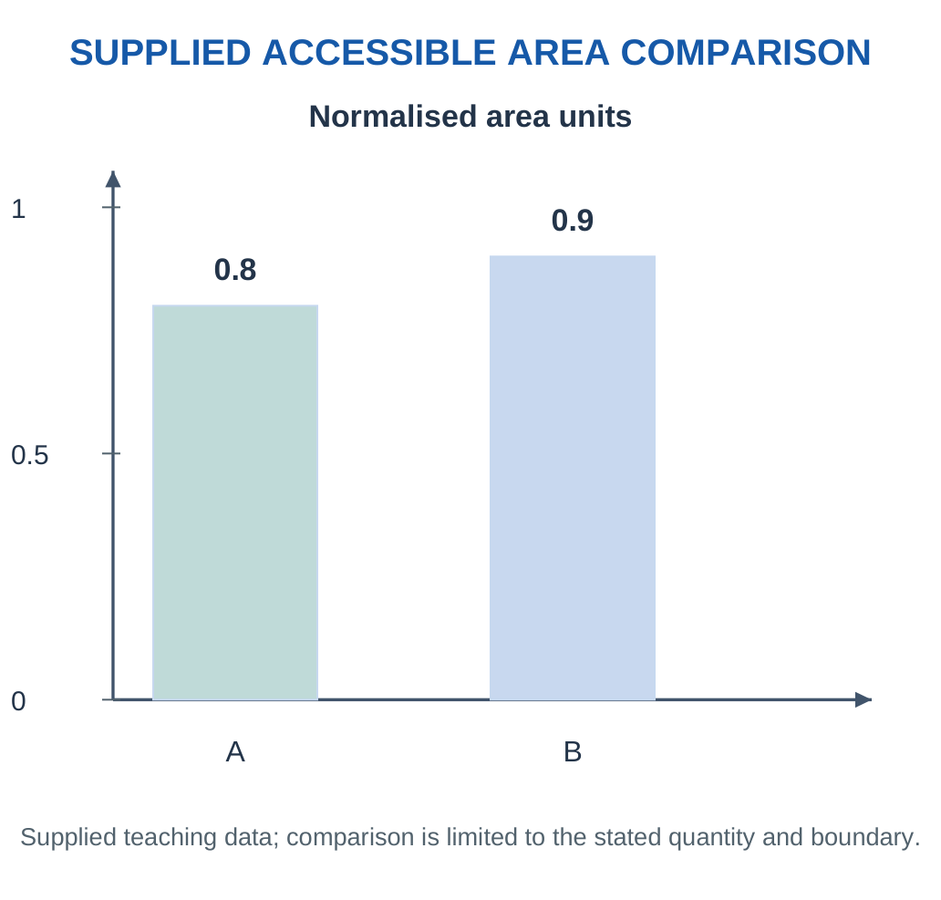
Two equal-mass spherical powders have the same density. Powder A has nominal diameter 20 nm, while B has 40 nm. A supplier reports that only 40% of A’s ideal geometric area is accessible in the proposed liquid, compared with 90% for B. These fractions are supplied teaching data, not general properties of the particle sizes.
Step 1: Compare Ideal Areas.
At equal mass and density, ideal area varies inversely with diameter. Choose B’s ideal area as one arbitrary area unit. A then has two ideal area units.
Step 2: Apply Access Fractions.
- A’s accessible area = 2 × 0.40 = 0.80 units
- B’s accessible area = 1 × 0.90 = 0.90 units
Despite its larger nominal particles, B provides more accessible area under these supplied conditions.

Step 3: Interpret the Result.
B has 0.90/0.80 = 1.125 times A’s accessible area, or 12.5% more on this model. This does not establish a 12.5% improvement in a sensor response or reaction rate. Per-area chemistry, transport and device construction also matter.
Step 4: Identify Useful Next Evidence.
Measure the functional response in the actual medium and check dispersion stability over the required time. If A improves after a dispersion treatment, reassess both access and the required electrical/chemical property; the treatment can change more than one variable.
Workshop Conclusion: Smaller nominal size supplies an ideal geometric advantage, but the engineering choice follows accessible interfaces and measured function. The comparison basis and medium must remain explicit.
Worked Example 4.1: Surface-to-Volume Scaling
Problem: Compare isolated spherical particles of diameters 20 and 100 nm. Find A/V in m⁻¹ and the area ratio for equal total volume.
Model / Approach: Smooth spheres; all geometric area accessible and no aggregation.
Step 1: Convert d to 2 × 10⁻⁸ and 1 × 10⁻⁷ m.
Step 2: Use A/V = 6/d:
- For 20 nm: A/V = 3 × 10⁸ m⁻¹
- For 100 nm: A/V = 6 × 10⁷ m⁻¹
Step 3: The ratio is 5:1 for smaller versus larger particles.
Step 4: At equal total solid volume, ideal exposed area is five times greater for the 20 nm population. The relation does not independently calculate reaction rate.
Answer: 3 × 10⁸ and 6 × 10⁷ m⁻¹; ratio 5:1.
Check and Interpretation: Smaller equal-shape particles have greater geometric area per volume.
Worked Example 4.2: Subdivision with Conserved Material
Problem: A 1 μm cube is divided into 1000 separate equal cubes. Find new side and total area ratio.
Model / Approach: Complete separation exposes all new faces; no volume is lost.
Step 1: There are cube-root(1000) = 10 divisions along each edge.
Step 2: Small side = 1/10 μm = 100 nm.
Step 3: New total area = 1000 × 6(L/10)² = 10 × original area.
Step 4: Volume remains 1000(L/10)³ = L³. If the pieces remained bonded, their internal faces would not count as exposed.
Answer: Small side 100 nm; exposed area increases tenfold.
Check and Interpretation: Volume is unchanged while exposed area grows.
Worked Example 4.3: Specific Area on a Mass Basis
Problem: A batch contains 2 g of smooth spherical particles of diameter 50 nm and density 2000 kg/m³. Estimate total exposed geometric area. Compare the same mass at 100 nm.
Model / Approach: Use A/m = 6/(ρd), fully exposed spheres and no porosity or aggregation. Density is supplied and unchanged.
Step 1: Convert mass to 0.002 kg and diameter to 5 × 10⁻⁸ m. Keeping density in kg/m³ ensures the area-to-mass result is m²/kg.
Step 2:
Specific area = 6/(2000 × 5 × 10⁻⁸) = 60000 m²/kg
Total area = 0.002 × 60000 = 120 m²
Step 3: At 100 nm, the diameter doubles, so specific area halves to 30000 m²/kg and total area becomes 60 m². The equal-mass ratio is 2:1.
Step 4: The result describes ideal geometric exposure. If particles cluster, some surface becomes inaccessible, and an adsorption measurement need not equal this simple estimate. A larger area also does not independently specify chemical reaction rate.
Answer: Ideal total area 120 m² at 50 nm; 60 m² at 100 nm.
Check and Interpretation: The units reduce to m², and doubling diameter halves area at fixed mass and density.
2. Dimensionality and Quantum Confinement
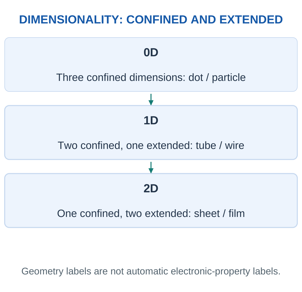
The labels 0D, 1D and 2D count extended dimensions. All physical specimens still have length, width and thickness.
| Class | Geometry and Example |
|---|---|
| 0D | All three dimensions confined; nanoparticle or quantum dot |
| 1D | Two confined dimensions, one extended; nanotube or nanowire |
| 2D | One confined thickness, two extended directions; graphene or nanosheet |
| Nanostructured bulk | Large specimen containing nanoscale grains, pores or phases |

Surface Fraction
A geometric estimate treats an outer shell of thickness δ as the surface region of a sphere. Its volume fraction is:
f = 1 − (1 − 2δ/d)³
The model requires 0 ≤ 2δ ≤ d.
It is an outer-shell estimate, not an exact count of surface atoms. Surface coating and particle contacts can change the exposed chemistry.
Electronic Confinement
When a relevant electronic length scale becomes comparable with a particle dimension, allowed states can differ from those in an extended crystal. In suitable semiconductor quantum dots, smaller size can increase the effective gap and shift emission towards shorter wavelengths. Composition, defects, shape and surface states also matter.
Common Error: Large surface area and quantum confinement are different ideas. A powder can have strong surface effects without useful visible emission. Not every nanoparticle is a quantum dot.
Key Point: Confined Is Not Extended
A wire has one extended direction and two confined directions, so it is geometrically 1D. A sheet has two extended directions. The class label does not independently prove an electronic band gap or a particular emission colour.
Why Dimensions Affect Electron Motion
In an extended solid, electrons occupy states determined by the material and its large-scale periodic structure. Restricting motion over a sufficiently small region can change the permitted states. A useful introductory analogy is a standing wave: the boundaries permit only certain patterns. The analogy explains discrete allowed modes; it does not mean that an electron is a visible vibrating string.
A small dimension alone does not establish strong confinement. The dimension must be compared with the relevant electronic length scale for that material and state. Temperature, disorder and interactions also influence what is observed. This is why different nanomaterials should not be assigned the same optical law.
Surface and Confinement Can Coexist
A quantum dot can simultaneously have a large surface fraction and confined electronic states. Surface defects can reduce emission even when confinement produces a suitable transition energy. A shell or ligand treatment can change losses without changing the simple geometric diameter in the same way as a size-controlled synthesis.

Classification Practice with Reasoning
A film with nanoscale thickness and millimetre-scale lateral dimensions is geometrically 2D. A nanoscale particle embedded inside that film remains a 0D inclusion. The device therefore need not fit into one single geometry label. State the level being described: particle, film, network or complete assembly.
Better Wording: “The dot confines carriers in three directions under the relevant material conditions” is more informative than “it glows because it is very small”.
Worked Example 4.4: Surface-Shell Fraction
Problem: Use shell thickness δ = 0.5 nm for a 10 nm spherical particle. Find the shell volume fraction.
Model / Approach: Use the geometric model f = 1 − (1 − 2δ/d)³, not an exact surface-atom count.
Step 1: Interior diameter = 10 − 2(0.5) = 9 nm.
Step 2: Interior volume fraction = (9/10)³ = 0.729.
Step 3: Shell fraction = 1 − 0.729 = 0.271.
Step 4: Thus 27.1% lies in the specified outer shell. Atoms there need not have identical chemistry or environmental access.
Answer: Shell fraction 27.1%.
Check and Interpretation: The shell thickness is smaller than the particle radius.
Worked Example 4.5: Classify Confined Directions
Problem: Classify sizes 8 × 8 × 8 nm, 8 × 8 × 5000 nm and 1 × 2000 × 2000 nm.
Model / Approach: Use geometry, not an assumed electronic property.
Step 1: The particle has no extended direction: 0D.
Step 2: The long wire has one extended direction: 1D.
Step 3: The sheet has two extended directions: 2D.
Step 4: All three objects have physical volume. Classification alone does not establish fluorescence, metallic conduction or a band gap.
Answer: 0D particle; 1D wire; 2D sheet.
Check and Interpretation: Count extended dimensions rather than simply counting the nanoscale dimensions.
3. Preparation, Dispersion and Characterisation
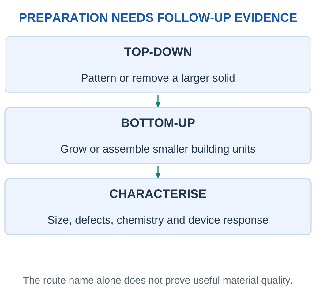
A top-down route creates small features from a larger solid by patterning, removal or subdivision. A bottom-up route builds from smaller chemical units through nucleation, growth, deposition or assembly. The route name does not prove purity, uniformity or device performance.

Control the Interfaces
Particles can aggregate through attractive interactions. Surface functionalisation can improve compatibility with a solvent or polymer, but the same chemical treatment may alter charge transfer or optical response. A composite needs suitable dispersion and interfacial bonding, not simply a specified filler mass.
A size distribution can broaden a material’s response. A reported mean should therefore be accompanied by appropriate sampling and spread information when the distribution matters. Processing can also introduce defects, residues or damage.
| Question | Evidence Needed |
|---|---|
| Size and shape? | Calibrated microscopy with representative sampling |
| Crystal structure? | Diffraction and complementary structural analysis |
| Surface chemistry or defects? | Suitable spectroscopy and material model |
| Useful conduction or emission? | Electrical or optical testing under stated conditions |
Photograph Versus Measurement
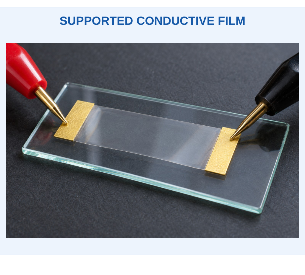
A photograph can show a film, supported coating or assembled device. It cannot prove graphene layer count, CNT chirality or a quantum-dot diameter. Use appearance illustrations for context and analytical evidence for nanoscale claims.
Link the Steps: Preparation → structure and interfaces → measured property → device function. Explain a causal link rather than listing methods without their purpose.
Select a Preparation Route by the Needed Feature
Top-down patterning can place features at defined positions on a substrate, which matters for a device contact or circuit. Bottom-up growth can create material through controlled chemistry but still requires suitable placement, purification and interfaces. A method that produces many particles is not automatically a method that produces a working transistor or display layer.
Choose the Measurement Before Naming an Instrument
A microscope image should include scale calibration and representative sampling. An electrical test should state geometry, contacts and conditions. A spectrum should state the excitation or observation range and relevant background treatment. If one measurement changes, ask whether the material, interface or test conditions changed.
Characterisation Logic: Structure supports an explanation, but performance needs a functional measurement. Conversely, a low resistance does not identify which nanoscale structure caused it.
Growth, Nucleation and Distribution: An Introductory View
Nucleation creates small stable regions of a new phase; growth increases their size. If nuclei form over a long interval, early particles may grow longer than late ones, creating a broad size distribution. Separating or controlling these stages can help obtain a narrower distribution. Actual behaviour depends on the chemistry, transport and process conditions.
Temperature and reactant availability influence rates, but a higher temperature does not universally give smaller particles. Faster nucleation, faster growth and aggregation can compete. A correct first-year explanation describes the competing stages rather than asserting one direction without a stated system.
Dispersion Is More Than Stirring
A dispersion must resist unacceptable settling or clustering over its required processing and use time. Surface groups, solvent compatibility and particle interactions influence this stability. A mixture that looks uniform immediately after mixing can change later. A film printed from an unstable ink can therefore show non-uniform thickness and resistance.


Choosing Evidence for a Claim
A claim of narrower particle size needs representative size data. A claim of improved conductivity needs matched electrical tests. A claim of better stability needs observations over an appropriate interval. One favourable observation should not replace the specific measurement the claim requires.
Practical Answer Example
A conductive ink becomes less stable after a surface treatment. The treatment may have changed particle-medium compatibility even if it improved the intrinsic conductivity of individual particles. The film result combines particle properties, dispersion, drying and contacts. Evaluating these links explains why material processing is part of device chemistry.
Worked Example 4.6: Composite Loading on a Final-Mass Basis
Problem: A 25 g dry composite needs 0.8% CNT by mass. Find CNT and polymer masses.
Model / Approach: The percentage refers to final dry composite, with no remaining solvent or other additive.
Step 1: Convert 0.8% to 0.008.
Step 2: CNT mass = 25 × 0.008 = 0.200 g.
Step 3: Polymer mass = 25 − 0.200 = 24.800 g.
Step 4: The masses sum to 25.000 g. Composition alone does not establish dispersion or a percolating network.
Answer: CNT 0.200 g and polymer 24.800 g.
Check and Interpretation: Using polymer alone as denominator would describe another loading convention.
Worked Example 4.7: Use an Average Without Hiding Distribution
Problem: Two supplied batches each have five particle diameters:
- A: 18, 19, 20, 21, 22 nm
- B: 10, 15, 20, 25, 30 nm
Compare means and ranges.
Model / Approach: Treat the listed measurements as illustrative complete datasets; do not infer a population distribution or exact optical spectrum.
Step 1: For A, the sum is 100 nm and mean is 100/5 = 20 nm. The minimum is 18 and maximum 22, giving a 4 nm range.
Step 2: For B, the sum is also 100 nm and mean is 20 nm. Its minimum is 10 and maximum 30, giving a 20 nm range.
Step 3: The equal means therefore hide a fivefold difference in the observed ranges. A is the narrower supplied size set, even though the central arithmetic value matches.
Step 4: A size-sensitive optical response may be influenced by the distribution, but its spectrum cannot be calculated from the range alone. Composition, shape, defects and surface state also need consideration.
Answer: Both means 20 nm; ranges 4 nm for A and 20 nm for B.
Check and Interpretation: A mean is one summary statistic. Reporting only 20 nm for both would omit an important observed difference.
4. Carbon Nanotubes: Structure and Properties
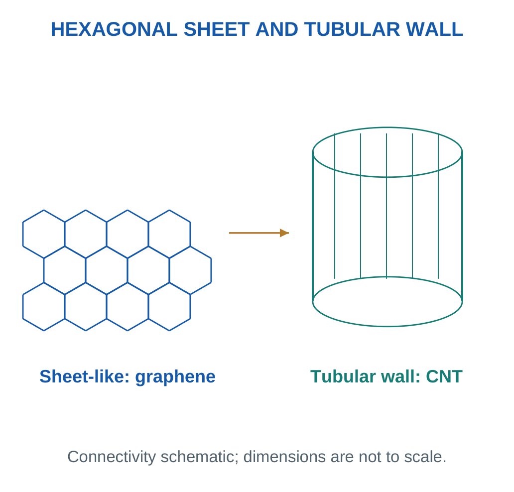
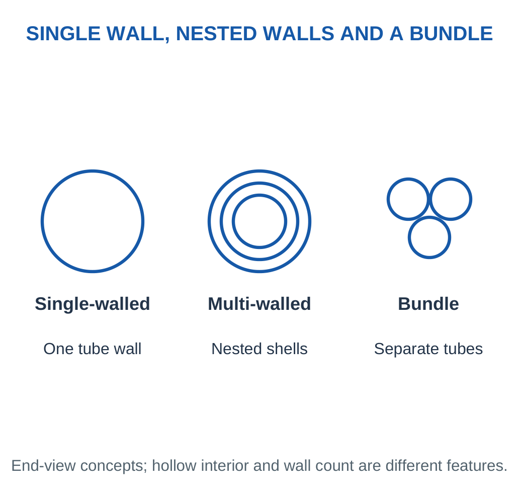
A carbon nanotube (CNT) has a cylindrical graphitic wall. A single-walled CNT has one tubular wall, while a multi-walled CNT contains nested walls. A bundle of separate tubes is different from one multi-walled tube.

Bonding and Conduction
The ideal wall contains an sp²-bonded carbon network. Strong in-plane bonding contributes to axial stiffness, and delocalised electronic states support useful transport. Single-walled CNT electronic behaviour depends on structure, including chirality and diameter; different tubes can be metallic or semiconducting.
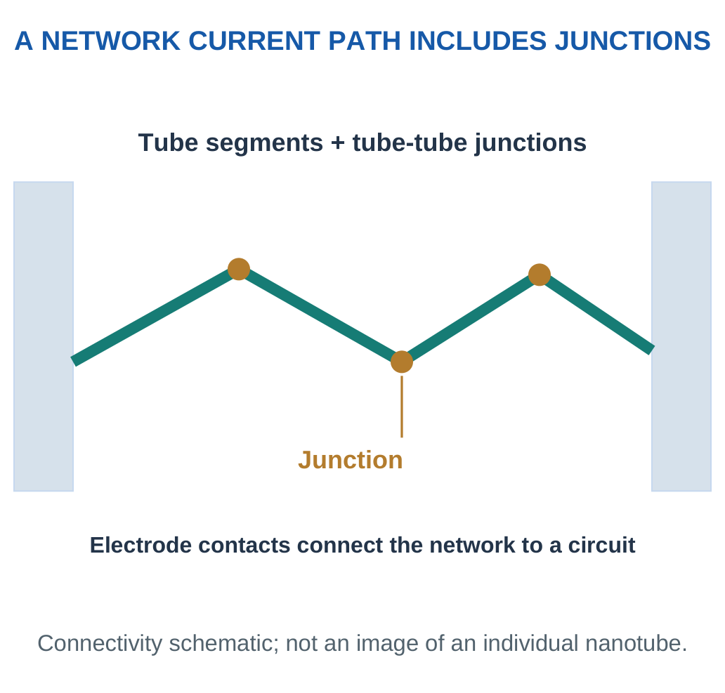
In a real film, tube-tube junctions, contacts, defects, impurities and processing damage can dominate resistance. Properties of one ideal tube are not automatically the properties of a bulk composite.
Reinforcement and Heat Transport
High-aspect-ratio fillers can reinforce a polymer and support heat or charge transport. Reinforcement requires effective stress transfer at the interface. Poorly dispersed clusters can instead introduce defects, while excessive filler can reduce flexibility or processability.
| Desired Benefit | Practical Limitation |
|---|---|
| Conductive network | Junction resistance and dispersion |
| Flexible electrode | Adhesion and repeated-bend stability |
| Responsive surface | Drift and non-target adsorption |
| Reinforcement | Interface quality and agglomeration |
Complete Answer: Draw single- and multi-walled concepts, describe bonding, state structure-dependent conduction and connect an application to its processing limitation.
Single-Walled and Multi-Walled Concepts
A single wall provides one tubular graphitic network. Multiple nested walls create several concentric shells, with inter-wall interactions and defects contributing to behaviour. Outside diameter, inside hollow diameter, wall number and tube length describe different features. A bundle contains several separate tubes held together and should not be labelled as one tube with many walls.

For a single-walled tube, chirality describes how the carbon network is oriented around the circumference. This structural arrangement helps determine electronic behaviour. For an introductory answer, it is enough to state that geometry and structure can produce metallic or semiconducting behaviour; do not assign every manufactured tube one identical conductivity.
From Filler to Reinforcement
The polymer must transfer stress into the filler through the interface. Poor bonding allows sliding; clustering can leave weak regions. An attractive axial property of an individual tube therefore needs good dispersion and interface design before it benefits a macroscopic component.
Chirality Without Unnecessary Mathematics
The hexagonal carbon network can meet around a tube circumference in different orientations. These arrangements are described through chirality. Common structural descriptions include armchair, zigzag and chiral forms. Their importance is that geometry affects electronic states; the names are not merely decorative shape labels.
A detailed electronic classification requires the actual tube indices and model. At this level, retain the central rule: some single-walled tubes are metallic and others semiconducting, while real specimens can contain a mixture. A conducting bundle does not prove that every tube inside it has identical electronic character.
Axial Versus Transverse Properties
Along the wall, strong carbon bonding supports a different transport and mechanical environment from motion across tube contacts. A network of short tubes can contain many junctions in the current path. Reducing the number or resistance of those junctions may improve a film even without improving the intrinsic tube material.

Open Ends, Defects and Functional Groups
Ends, structural defects and attached groups can provide chemically different sites. They can improve bonding to a matrix or interaction with an analyte. Excessive damage can disrupt transport or mechanical continuity. Functionalisation should therefore be assessed against the intended role, not described as automatically beneficial.
An Examination Comparison
For reinforcement, discuss stress transfer and dispersion. For an electrode, discuss contact network and continuity. For a sensor, discuss a reversible input-related response and interference. The same carbon structure can participate in all three applications, but each answer requires a different performance test.
Worked Example 4.8: Tube Aspect Ratio
Problem: A tube is 2 μm long with outside diameter 10 nm. Find length/diameter.
Model / Approach: Use the given straight length and outside diameter; wall count is not supplied.
Step 1: Convert 2 μm to 2000 nm.
Step 2: Aspect ratio = 2000/10.
Step 3: The ratio is 200, without units.
Step 4: A high aspect ratio can support network formation, but orientation, contacts and dispersion still determine the composite response.
Answer: Aspect ratio 200.
Check and Interpretation: Match length units before taking the ratio.
5. CNT Networks, Percolation and Sensing
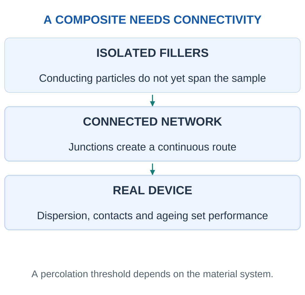
A polymer containing a few isolated conducting tubes may remain poorly conducting. Increasing connectivity can create a continuous route across the specimen. This development of a spanning network is electrical percolation. Its threshold depends on filler aspect ratio, orientation, dispersion and contacts; there is no universal loading percentage.
Key Point: A Network Can Respond to Several Inputs
Strain, temperature, humidity and adsorption can all change a composite resistance. A measured electrical response needs calibration and relevant controls before it is assigned to one input.



Resistance as a Signal
Stretching can change tube contacts or tunnelling distances and therefore resistance. Chemical adsorption can also alter a network response. A strain sensor must separate its desired mechanical input from temperature, humidity and chemical effects.
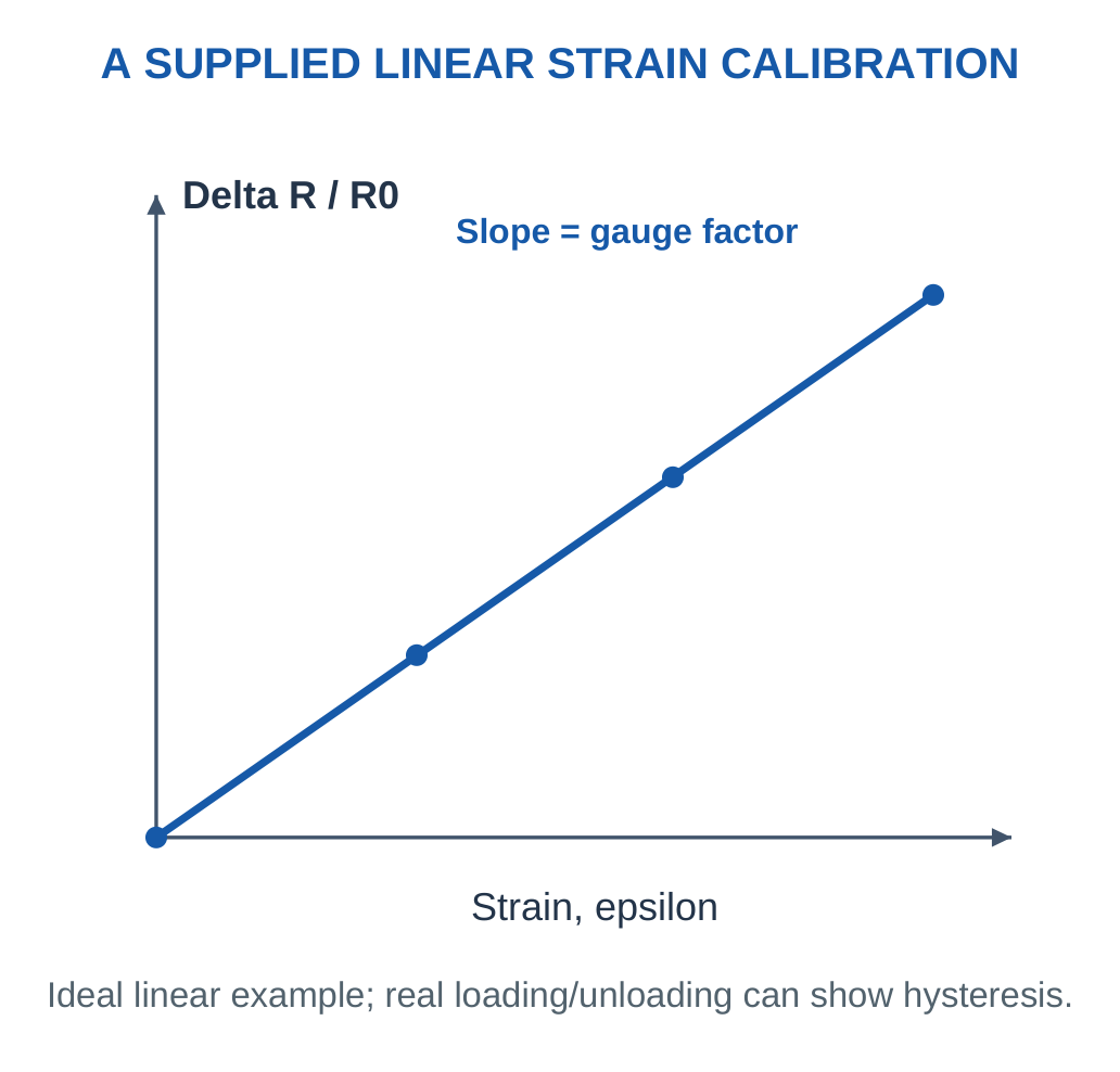
For a defined linear piezoresistive model:
GF = (ΔR/R₀)/ε
Here:
- R₀ = baseline resistance
- ΔR = signed resistance change
- ε = dimensionless strain
A 1% strain is 0.01 in the equation. Hysteresis, drift and irreversible damage require their own evaluation.
Applications
CNT composites and films are used or investigated for flexible conducting paths, strain sensing, antistatic surfaces and responsive electrodes. More filler can lower resistance while reducing transparency or flexibility. Encapsulation can improve durability but obstruct access of an analyte to a sensing interface.
Interpretation Trick: Name the input, baseline, sign of the resistance change and supported range. “Resistance changes” is an incomplete sensor explanation.
Reversible Response Versus Damage
A useful strain sensor changes its signal reproducibly when strain is applied and removed. A cracked conductor may also change resistance, but that change can be irreversible and unsuitable for repeated measurement. Loading and unloading curves reveal hysteresis, while repeated zero-input checks reveal baseline drift.
A calibration should specify its strain interval and measurement condition. If the network is also temperature-sensitive, a temperature change can imitate strain. A reference element, temperature measurement or appropriate compensation may help, but its effectiveness must be demonstrated.
Why More Filler Is Not Always Better
Higher loading can create more conducting contacts while reducing transparency, flexibility or print quality. A sensing network may need a large reversible fractional change rather than simply the lowest possible resistance. Match the chosen composition to the output and operating range.
Reading a Strain-Response Curve
A calibration plot should identify strain on the horizontal axis and a defined response such as ΔR/R₀ on the vertical axis. Its slope in a stated linear interval is the gauge factor under that model. A curved response requires an interval-dependent or other supported relation; one slope should not be applied far outside its calibration.
Loading and unloading can follow different paths. That difference is hysteresis and can affect how one resistance value maps back to strain. A slowly changing zero-strain resistance is drift. A resistance that fails to return after the specimen is unloaded may indicate permanent rearrangement or damage.

Network Design for a Repeated Sensor
A useful network should respond enough for the readout to distinguish the signal while remaining stable and recoverable. Very low resistance is not the sole objective. If a loading produces almost no fractional response, it may be a good conductor but a weak strain-sensing choice. If a sparse network breaks irreversibly, its large change may not be a repeatable sensor signal.
Pattern for an Application Answer
The input deforms the matrix; network contacts change; resistance changes; a readout measures that change; a calibration returns strain. Temperature and other mechanical directions can influence the chain. Each arrow should name a physical stage. Merely listing CNT, polymer and wireless module does not explain the measurement.
Worked Example 4.9: Strain Gauge Response
Problem: A strip has R₀ = 200 Ω and GF = 5. Find resistance at 1.5% tensile strain when R increases linearly.
Model / Approach: Use ΔR/R₀ = GFε; temperature and contacts unchanged in the supplied range.
Step 1: Convert ε = 0.015.
Step 2: ΔR/R₀ = 5 × 0.015 = 0.075.
Step 3: ΔR = 200 × 0.075 = 15 Ω.
Step 4: R = 215 Ω. A humidity change or damaged contact would require a different interpretation from this calibrated strain response.
Answer: ΔR = 15 Ω; final R = 215 Ω.
Check and Interpretation: (215 − 200)/200 gives 0.075, as required.
Worked Example 4.10: Read a Network-Transition Dataset
Problem: Loadings 0.1, 0.3, 0.5 and 0.8 wt% give resistances 10⁸, 10⁷, 10⁴ and 10³ Ω for identical specimens. Locate the sharpest drop.
Model / Approach: Compare adjacent supplied points; do not fit an exact threshold without more data.
Step 1: First interval gives a tenfold drop.
Step 2: The 0.3–0.5 wt% interval gives a thousandfold drop.
Step 3: The final interval gives a tenfold drop.
Step 4: The strongest observed transition is therefore 0.3–0.5 wt%. An exact threshold at the midpoint has not been measured.
Answer: Sharpest observed drop: 0.3–0.5 wt%, by 1000 times.
Check and Interpretation: An observed interval is justified; a precise universal threshold is not.
6. Graphene and Related Carbon Films
Graphene is one atomic layer of carbon in a two-dimensional hexagonal network. Its sp² bonding and electronic structure provide a useful combination of in-plane strength, electrical transport, thinness and optical transmission under suitable conditions.
Key Point: Graphene Oxide Is a Different Material
Oxygen-bearing groups and disrupted structure change processing and conduction. Reducing graphene oxide can improve conductivity without restoring every feature of a pristine monolayer.

Practical Distinctions
Graphite is a stacked bulk material. Few-layer graphene is not the same specimen as a monolayer. Graphene oxide contains oxygen-bearing groups and structural disruption that can improve processing in some media while reducing conductivity. Reduction can increase conductivity but does not necessarily restore a perfect graphene lattice.
Ideal monolayer graphene has no conventional band gap. This helps explain why its useful conduction does not make it a universal replacement for silicon digital switches: suppressing the off-state current is a different requirement from making a good conducting film.

Device Roles
Graphene-containing materials can serve as transparent electrodes, conductive inks, sensing interfaces and composite fillers. Defects, grain boundaries, residues, film continuity and contact quality control real performance. A transparent conductor must satisfy optical and electrical requirements together.
Compare with CNTs: Graphene is sheet-like, while a CNT has a tubular wall. Both contain related carbon bonding networks but differ in geometry, processing and contacts.
Electrode and Sensing Roles Are Distinct
As an electrode, a graphene-containing film should carry charge with acceptable loss. As a sensing interface, interaction with the environment may intentionally alter a measured property. The same environmental sensitivity that helps sensing can be a source of instability in an electrode.
Contacts and Substrate Effects
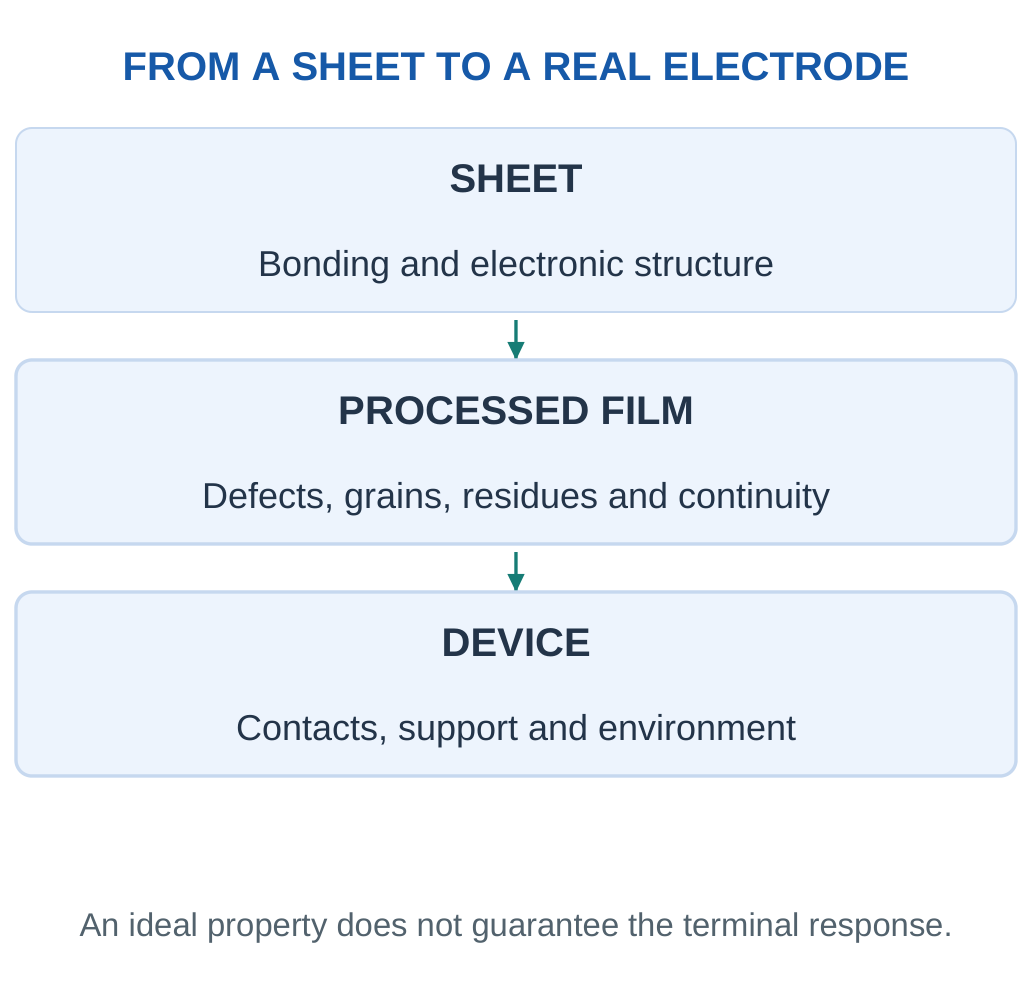
An electrode film needs a path into the external circuit. A poor metal-film interface can add resistance or unstable behaviour. Support layers can introduce stress, contamination or charge effects. A reported material property should therefore state whether it concerns an isolated ideal sheet, a processed film or a complete terminal measurement.

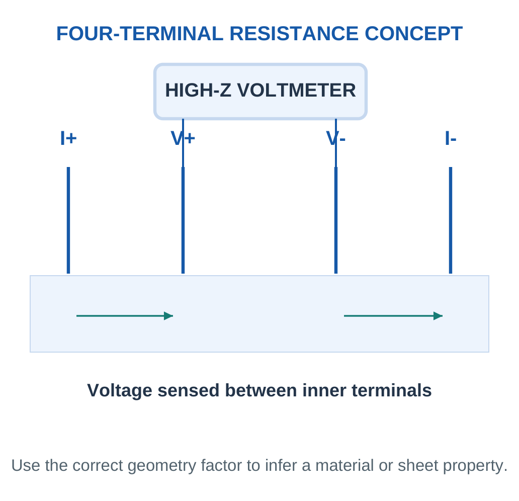
The four-terminal idea reduces selected lead/contact voltage contributions. It does not automatically repair a cracked film, remove non-uniformity or determine a sheet-resistance value without the correct geometry.
Transparency and Film Continuity
A very thin carbon layer can transmit substantial light, which motivates transparent electrodes. The practical film must also provide a continuous route between contacts. Tears or incomplete coverage can increase resistance even when much of the substrate remains transparent. Optical transmission and electrical continuity therefore need separate evidence.
For a processed film made from flakes, overlap and junctions between flakes affect conduction. A flake film and a high-quality continuous monolayer are different material systems. The word graphene alone does not specify either construction.
Adsorption and Sensing
When a surface interaction changes an electrical response, a graphene-based structure may serve as a sensing interface. The measurement still needs selectivity and relevant environmental controls. A large response to a target does not show that another species produces no response. Surface treatment and encapsulation can change access to the active region.
Compare Three Carbon Forms
| Form | Structural Distinction | Practical Question |
|---|---|---|
| Graphene | Sheet-like carbon layer | Is the processed film continuous and well contacted? |
| Graphene oxide | Oxygen-bearing, disrupted structure | Is processing compatibility worth the altered conduction? |
| Reduced graphene oxide | Partly restored conductivity after reduction | Which defects and groups remain? |
The comparison is qualitative. Different preparation routes can produce different specimens within each name. Use an actual measured property for a device decision rather than assigning one universal resistance to an entire material family.
Worked Example 4.11: Find Sheet Resistance
Problem: A uniform film reads 240 Ω film-only resistance, with length 12 mm and width 3 mm. Find Rₛ.
Model / Approach: R = RₛL/W; ignore contact and edge effects.
Step 1: Number of squares L/W = 12/3 = 4.
Step 2: Rearrange Rₛ = R/(L/W).
Step 3: Rₛ = 240/4 = 60 Ω per square.
Step 4: A square specimen of the same uniform film gives 60 Ω between the specified opposite edges in this ideal geometry.
Answer: 60 Ω per square.
Check and Interpretation: Four squares in series reproduce 240 Ω.
7. Sheet Resistance and Transparent Electrodes
For a uniform rectangular thin film:
R = RₛL/W
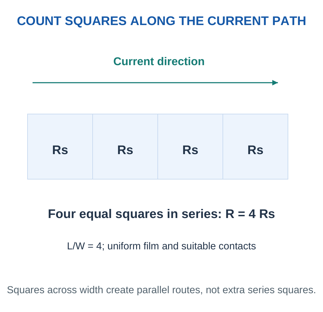
Here Rₛ is sheet resistance and L/W is the number of squares. The ratio is dimensionless. Doubling both length and width leaves this ideal resistance unchanged.
The model assumes suitable contacts, uniform thickness and a simple current path. Real two-terminal resistance can include contact and lead contributions. Cracks and non-uniform films can invalidate a simple geometry estimate. An appropriate four-terminal measurement reduces certain contact/lead contributions.
Electrical and Optical Trade-Off
Optical transmission is I/I₀ for a stated wavelength or spectrum. Low resistance is useful for charge transport, but a display electrode also needs sufficient transmission and acceptable haze. Adding more conducting material can improve resistance while reducing transparency.
| Requirement | Evidence |
|---|---|
| Charge transport | Sheet resistance, contacts and uniformity |
| Optical function | Transmission spectrum and haze |
| Flexibility | Electrical behaviour through bend cycles |
| Stability | Adhesion, moisture resistance and ageing |
Quick Checks:
- At fixed width and sheet resistance, doubling length doubles R.
- At fixed length, doubling width halves R.
- A long narrow track can have significant voltage drop despite an attractive sheet-resistance value.
A useful selection starts with actual limits: for example, a maximum resistance and a minimum transmission. Pass both before ranking durability, cost or processing compatibility.
Deriving the Number-of-Squares Relation
For a uniform conductor:
R = ρL/A
A rectangular film has cross-sectional area A = Wt, where t is thickness.
Therefore:
R = (ρ/t)(L/W)
Defining sheet resistance Rₛ = ρ/t gives:
R = RₛL/W
This derivation explains why sheet resistance captures the material/thickness term while L/W captures planar geometry.
The derivation assumes a uniform material and a suitable current distribution. It cannot automatically describe a patterned film with narrow necks, cracks or strongly varying thickness. A device drawing should show the direction of current and which edges act as contacts.

Voltage Drop and Heating
A current I through film resistance R produces:
- Voltage drop = IR
- Electrical power = I²R
A conductor chosen for low signal loss should therefore be assessed at the actual operating current. A resistance acceptable for a high-input-impedance measurement can be unsuitable for a power path.
Temperature and Stability
Material resistivity can change with temperature, and a processed network can also change through contact rearrangement. Comparing a film before and after heating needs matched measurement conditions. A low room-temperature resistance is not a complete thermal or reliability specification.
Unit Discipline: ρ in Ω·m and t in m give Rₛ in Ω per square. L/W has no unit; writing an extra length unit after the final resistance indicates a geometry error.
Guided Design: Geometry Can Dominate a Conductive Path
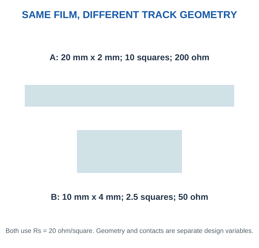
A uniform film has sheet resistance 20 Ω per square. Path A is 20 mm long and 2 mm wide. Path B is 10 mm long and 4 mm wide. Both use the same film and thickness, with suitable contacts and no additional series contribution in this model.
Path A: L/W = 10 squares, so resistance is 200 Ω.
Path B: L/W = 2.5 squares, so resistance is 50 Ω.
The material is unchanged, yet the geometry gives a fourfold resistance difference.

Same Resistance Does Not Mean Same Construction
An alternative material or thickness can change sheet resistance, while layout changes L/W. Several combinations can produce one terminal resistance. A measured 50 Ω therefore does not uniquely identify the film composition, thickness or track dimensions. Additional information is needed to infer those properties.
Series and Parallel Logic
Two identical 50 Ω tracks connected in series give 100 Ω under the ideal circuit model. Two connected in parallel between the same nodes give 25 Ω if current shares symmetrically. A physical drawing must show the actual contact nodes; merely drawing nearby squares does not prove an electrical parallel connection.
Key Point: Count Squares Before Using a Film Formula
The ratio L/W is dimensionless and independent of the chosen common length unit. Contact resistance is a separate terminal contribution; a film-only estimate should not silently become a complete device-resistance specification.
Application Interpretation
A sensor interface can benefit from a geometry chosen for measurable resistance, while an interconnect can need low voltage drop. The objective differs even when the film material is shared. Narrowing a path can raise resistance but also create current crowding or mechanical weak regions in a real layout.
A complete device choice therefore considers film quality, contact design, track shape and the operating current. The number-of-squares relation is a useful starting model, not a replacement for checking the actual assembled path.
Design Check: When a calculation gives an unexpectedly large voltage drop, inspect both Rₛ and L/W before assuming the material property alone is wrong.
Worked Example 4.12: Size a Film Electrode
Problem: A film has Rₛ = 35 Ω per square and track length 20 mm. Find minimum width for film resistance ≤100 Ω.
Model / Approach: Uniform rectangle; terminal contact resistance is not included.
Step 1: Write 35 × 20/W ≤ 100.
Step 2: Rearrange W ≥ 35 × 20/100.
Step 3: Minimum model width = 7 mm.
Step 4: A real total-terminal limit must also allow for contacts and non-uniformity. This is only the film contribution.
Answer: Minimum model width 7 mm.
Check and Interpretation: At 7 mm width, film resistance is exactly 100 Ω.
Worked Example 4.13: Separate Contact Resistance
Problem: Two-terminal resistance is 150 Ω and independently known film resistance is 110 Ω. Two equal contacts contribute the rest. Find each.
Model / Approach: Use the supplied series model; lead contribution is neglected.
Step 1: Combined contacts = 150 − 110 = 40 Ω.
Step 2: There are two equal contacts.
Step 3: Each contributes 40/2 = 20 Ω.
Step 4: Improving the film alone would not remove this part of the terminal resistance. Other current geometries may need a more detailed model.
Answer: 20 Ω per contact.
Check and Interpretation: 110 + 20 + 20 = 150 Ω.
Worked Example 4.14: Connect Resistivity, Thickness and a Track
Problem: A uniform film has ρ = 2 × 10⁻⁶ Ω·m, thickness 100 nm, track length 10 mm and width 2 mm. Find sheet resistance and track resistance.
Model / Approach: Use a uniform rectangular film, Rₛ = ρ/t and R = RₛL/W. Contact and lead contributions are excluded.
Step 1: Convert thickness:
100 nm = 1 × 10⁻⁷ m
Rₛ = (2 × 10⁻⁶)/(1 × 10⁻⁷) = 20 Ω per square
Step 2: Use common planar units to find L/W = 10/2 = 5 squares. The ratio does not need separate conversion to metres.
Step 3: Track resistance = 20 × 5 = 100 Ω. A direct calculation with R = ρL/(Wt) gives the same film-only result.
Step 4: The model assumes continuous coverage and a suitable current path. A cracked or non-uniform film can deviate, and a two-terminal measurement can include additional contact resistance.
Answer: Sheet resistance 20 Ω per square; track resistance 100 Ω.
Check and Interpretation: Thickness is required in the resistivity relation, while L/W is a dimensionless ratio.
Worked Example 4.15: Voltage Loss and Heating in an Electrode
Problem: A film track has 100 Ω resistance and carries a constant 20 mA. Find voltage drop, electrical power and energy dissipated in 60 s.
Model / Approach: Use a fixed ohmic resistance and constant current. No thermal resistance or heat capacity is supplied, so temperature rise is outside the model.
Step 1: Convert current to 0.020 A.
Voltage drop = IR = 0.020 × 100 = 2.0 V
This must be considered in a device voltage budget.
Step 2:
Power = I²R = (0.020)² × 100 = 0.040 W
The alternative calculation VI gives 2.0 × 0.020 = 0.040 W.
Step 3:
Energy = Pt = 0.040 × 60 = 2.4 J
This is electrical dissipation in the stated resistance, not useful optical or mechanical output.
Step 4: Temperature depends on heat transfer, geometry and material properties. A low measured power does not automatically establish negligible temperature change in every thin-film device.
Answer: Drop 2.0 V; power 0.040 W; dissipated energy 2.4 J.
Check and Interpretation: The two power formulas agree, and multiplying watts by seconds gives joules.
8. Quantum Dots: Absorption, Emission and Colour
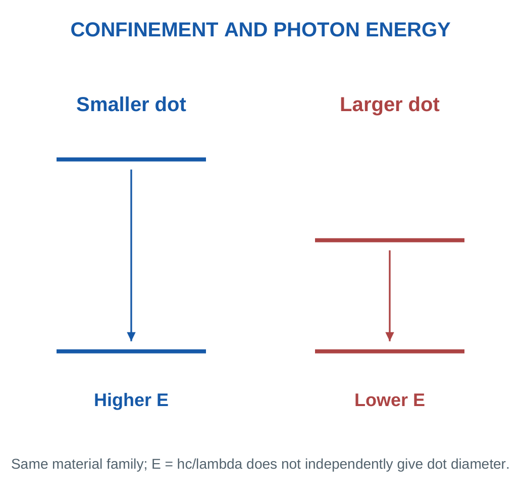
Quantum dots are semiconductor nanostructures that can confine carriers in all three directions. Their size-sensitive electronic states can produce a tunable optical response. Composition, size distribution, shape, core/shell design and surface chemistry all influence the spectrum.

From Excitation to Emission
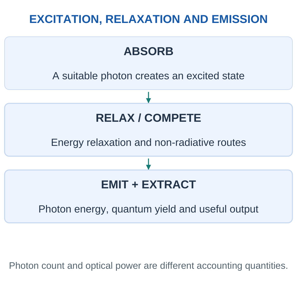
Suitable photons create excited states. Relaxation can be followed by radiative electron-hole recombination, producing an emitted photon. Non-radiative pathways compete with emission. Surface defects can create loss channels; passivation or a suitable shell can reduce selected surface-related losses.
For one photon:
E = hc/λ
Approximately:
E(eV) = 1240/λ(nm)
Shorter wavelength means higher photon energy. This converts energy and wavelength; it does not independently determine dot diameter.
Quantum Yield
Photoluminescence quantum yield is emitted photon count divided by absorbed photon count over a defined measurement. It differs from electrical efficiency, which includes electrical input and other system losses. Brightness also depends on excitation intensity, absorption and collection geometry.
| Quantity | Meaning |
|---|---|
| Excitation | Energy supplied to create an excited state |
| Emission peak | Wavelength region of strong emitted intensity |
| Spectral width | Spread around the peak |
| Quantum yield | Emitted photons per absorbed photon |
Avoid a Shortcut: Colour alone cannot establish composition, dot diameter, concentration or device efficiency. Interpret it with a supported material model.
Core, Shell and Surface Ligands
A core-shell dot has a central semiconductor region and a surrounding shell chosen to modify confinement or surface behaviour. Surface ligands help stabilise the particle in a medium and influence processing. Their chemistry can affect compatibility, charge transfer and stability.
Key Point: Photon Energy Is Not Dot Diameter
E = hc/λ converts wavelength and photon energy. Inferring dot size additionally needs a material-specific relation, including relevant composition and surface assumptions.

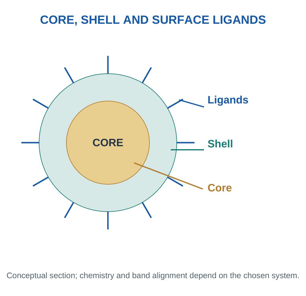
A shell can reduce certain surface-related losses, but strain, interface defects or unsuitable band alignment can introduce new limitations. Different dot systems therefore need their own optical characterisation rather than one universal shell explanation.
Ensemble Spectra
A collection of dots contains many emitters. A broad size distribution, different local environments or defects can broaden the measured output. The observed spectrum is an ensemble response, while one idealised energy-level sketch explains only the chosen mechanism. Distinguish a peak position from its width and total emitted intensity.
Excitation Energy and Emission Energy
An absorbed photon can excite a dot into an available higher-energy state. The system may lose part of that energy through relaxation before radiative emission. The emitted photon can therefore have lower energy and longer wavelength than the exciting photon. This qualitative picture separates excitation selection from the observed emission peak.
The photon relation E = hc/λ applies to each photon. A quantum yield counts photons, not the equality of absorbed and emitted energies. Even an idealised one-emitted-photon-per-absorbed-photon case can have an optical energy loss when emitted photons are lower energy.

Surface Losses and Passivation
A surface-related state can provide a non-radiative route or modify emission. Appropriate passivation can reduce some of these effects, but the result depends on the actual surface and shell chemistry. A well-protected particle can still degrade under unsuitable illumination or temperature.
Peak Position, Width and Intensity
Peak position describes where emission is concentrated in wavelength. Width describes its spread. Integrated intensity describes the amount collected under the measurement. These quantities can change independently. A narrow peak is not automatically a brighter sample, and a brighter sample is not automatically a higher-yield emitter if it absorbed more excitation light.
Worked Example 4.16: Photon Energy from Colour
Problem: Find photon energy for 450 nm and 620 nm emission.
Model / Approach: Use E(eV) = 1240/λ(nm).
Step 1: 450 nm gives 1240/450 = 2.756 eV.
Step 2: 620 nm gives 1240/620 = 2.000 eV.
Step 3: The shorter-wavelength photon is higher energy by about 0.756 eV.
Step 4: These conversions do not determine quantum-dot diameter without a material-specific relation. Composition and surface states also affect a real spectrum.
Answer: Approximately 2.76 eV and 2.00 eV.
Check and Interpretation: Energy must increase when wavelength decreases.
Worked Example 4.17: Wavelength from a Transition
Problem: A supplied optical transition emits a 2.4 eV photon. Estimate wavelength.
Model / Approach: Use λ(nm) = 1240/E(eV), not a dot-size model.
Step 1: The energy is already in the required eV unit.
Step 2: Rearrange λ = 1240/2.4.
Step 3: λ ≈ 516.7 nm.
Step 4: This is an optical energy conversion. It does not identify the semiconductor or its diameter.
Answer: Approximately 517 nm.
Check and Interpretation: 2.4 × 516.7 is approximately 1240 eV·nm.
9. Quantum Dots in Smart Displays
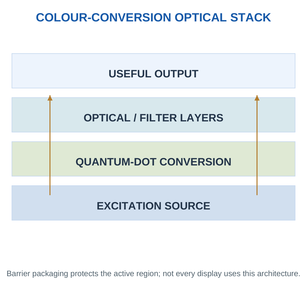
A colour-conversion display can use an excitation source and quantum-dot layer to produce selected output colours. Other architectures electrically excite quantum-dot layers. Optical colour conversion and direct electroluminescence are distinct arrangements.
Key Point: Efficiency Stage Matters
Absorption, emission quantum yield and extraction use different denominators. State which photons are counted at each stage before multiplying fractions or interpreting the result as a device efficiency.


The Complete Optical Stack
Source spectrum, absorption, quantum yield, extraction, filters and packaging influence the final output. A high material quantum yield is only one part of overall performance. Moisture, oxygen, heat and prolonged excitation can change behaviour, so protection and ageing tests matter.
Some quantum-dot systems contain elements requiring careful material assessment and controlled waste routes. Alternative compositions can address selected concerns but still need performance and environmental evaluation. “Nano” and “cadmium-free” do not individually certify a harmless complete product.
Explain a Device Clearly
Name the source, conversion or emitting layer, output spectrum and protective role of encapsulation. Then explain one loss mechanism and one material limitation. Do not infer power efficiency solely from an emitted-to-absorbed photon ratio.
Numerical Discipline: Sequential photon-number fractions multiply. For power efficiency, photon energies and electrical source conversion must also be included.
Distinguish Three Efficiencies
Absorption fraction asks how many incident photons are absorbed. Photoluminescence quantum yield asks how many photons are emitted per absorbed photon. Extraction asks how much emission reaches the useful output. Their product can describe a supplied photon-number chain, but a complete power calculation also uses photon energies.
A display additionally contains an electrical source and drive electronics. The electrical-to-optical conversion of that source is outside a material-only photoluminescence measurement. Reporting a large quantum yield as a complete wall-plug efficiency skips these stages.
Optical Design Checklist: Source wavelength, absorbing layer, emitted spectrum, losses, extraction, thermal conditions and protective packaging. Explain where a photon is lost before assigning an efficiency value.
Colour-Conversion Architecture in Detail
A source supplies excitation, a conversion region absorbs part of it, selected emission travels towards the output and filters/optical layers shape the final spectrum. Unabsorbed source light can also contribute if the architecture uses it. The desired balance depends on the colour channels and design.

Thermal and Barrier Design
Repeated excitation and nearby electronics can heat the optical region. Temperature can affect response and long-term stability. Barrier layers can reduce access of moisture or oxygen, but also add thickness, interfaces and manufacturing constraints. The complete optical/mechanical stack must be evaluated together.
Useful Test Sequence
Measure the source spectrum, absorption behaviour and emitted spectrum under defined excitation. Evaluate quantum yield with an appropriate measurement. Then assess output extraction and final device response. Repeat under relevant thermal and ageing conditions. This sequence prevents one favourable material number from being used as a substitute for a system test.
Material Trade-Off
An alternative dot composition may reduce one material concern while changing spectrum, yield or stability. A useful first-year answer gives the reason for considering the alternative and identifies the properties that must still be verified. It should neither assume that every quantum dot contains the same elements nor that a new composition removes every environmental concern.
Application Workshop: Diagnose a Dimmer Optical Output
Three otherwise comparable prototype conversion layers are tested under a supplied photon-count model. All receive one million excitation photons.
- A absorbs 70%, has quantum yield 80% and extraction 60%.
- B absorbs 60%, has yield 90% and extraction 80%.
- C absorbs 90%, has yield 60% and extraction 50%.
| Prototype | Absorbed Photons | Emitted Photons | Useful Output Photons |
|---|---|---|---|
| A | 700000 | 560000 | 336000 |
| B | 600000 | 540000 | 432000 |
| C | 900000 | 540000 | 270000 |
Step 1: Multiply each stage on its own inlet basis. The strongest absorber C does not give the greatest useful output. Its lower yield and extraction offset the initial capture.
Step 2: B gives the highest supplied useful count despite absorbing less than A or C. It produces 432000/336000 ≈ 1.286 times A’s useful photons. This is about 28.6% more output on the stated count basis.

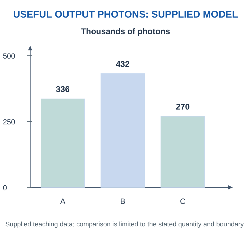
Step 3: Identify what the calculation omits. Equal photon counts do not ensure equal optical energy if output wavelengths differ. Electrical source losses, colour requirements, spectral width and ageing are also outside the simple count comparison.
Step 4: Diagnose a later dimming result by separating stages. A change in source intensity differs from reduced absorption, lower emission yield or poorer extraction. Measuring only the final brightness cannot identify which stage failed.
Workshop Conclusion: Follow the optical chain and preserve denominators. Select the device using required spectrum and stability as well as useful output under matched conditions.
Worked Example 4.18: Photoluminescence Quantum Yield
Problem: A layer absorbs 2.5 × 10⁶ photons and emits 1.8 × 10⁶. Find quantum yield.
Model / Approach: Counts refer to the same corrected measurement interval.
Step 1: Use emitted/absorbed photon count.
Step 2: Cancel the common 10⁶ factor.
Step 3: Φ = 1.8/2.5 = 0.72, or 72%.
Step 4: Electrical power efficiency and final display output include additional conversion stages and cannot be inferred from this ratio alone.
Answer: Quantum yield 72%.
Check and Interpretation: Photon count is the basis, rather than incident electrical energy.
Worked Example 4.19: Follow an Optical Photon Chain
Problem: Of 10⁶ incident photons, 60% are absorbed, 80% of absorbed photons produce emission and 75% of emitted photons reach output. Find output count.
Model / Approach: Treat all fractions as sequential photon-number fractions.
Step 1: Absorbed count = 600000.
Step 2: Emitted count = 600000 × 0.80 = 480000.
Step 3: Output count = 480000 × 0.75 = 360000.
Step 4: Overall photon-number fraction is 36%. A power-efficiency claim would also need photon energies and electrical source conversion.
Answer: 360000 output photons; 36% incident-to-output photon fraction.
Check and Interpretation: The three sequential fractions multiply to 0.36.
Worked Example 4.20: Photon-Number Yield Versus Optical-Energy Efficiency
Problem: A layer absorbs 100 photons of energy 3.0 eV each and emits 80 photons of energy 2.0 eV each. Find photon quantum yield and emitted-to-absorbed optical energy ratio.
Model / Approach: Use the supplied counts and photon energies, one measured interval and no extraction loss. Electrical-source efficiency is not supplied.
Step 1:
Photon quantum yield = 80/100 = 0.80 = 80%
The photon energy does not enter that count ratio.
Step 2:
- Total absorbed optical energy = 100 × 3.0 = 300 eV
- Total emitted optical energy = 80 × 2.0 = 160 eV
Step 3:
Optical-energy ratio = 160/300 = 0.5333 ≈ 53.3%
Lower emitted photon energy and incomplete photon emission both reduce the ratio.
Step 4: This is not a complete display wall-plug efficiency. The excitation source, electrical drive and extraction stage would add further parts to a system calculation.
Answer: Quantum yield 80%; optical-energy ratio approximately 53.3%.
Check and Interpretation: Equal photon counts would still not imply equal optical energy when photon energies differ.
10. Smart Coatings and Engineered Interfaces
A coating changes a surface property while a substrate provides much of the support. A smart coating supplies a useful response or adaptive function, such as a change in wetting, colour or protection under a stimulus. State the response rather than calling every protective paint smart.

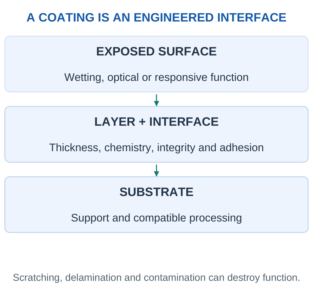
Design Variables
Thickness: More material can improve coverage but increase stiffness, optical loss or diffusion distance. A discontinuous film can leave unprotected regions.
Adhesion: Compatibility, preparation and thermal/mechanical stress influence long-term attachment. Good initial spreading during application does not guarantee durable adhesion.
Roughness: Texture can change apparent wetting and light scattering. A texture that helps water repellence may also produce haze or wear rapidly.
Durability: Evaluate scratching, repeated cleaning, moisture, temperature cycles and the intended environment. One attractive drop photograph is an initial observation, not a lifetime test.
Selection Rule: Choose the function and operating range first, then compare measured response, durability and compatibility. The best initial response can be unsuitable if it fails quickly.
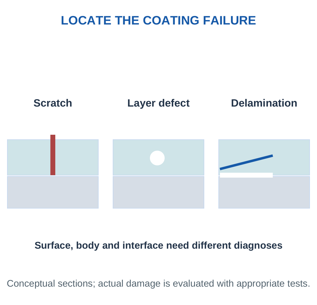
Coating Failure Can Start at Several Places
A scratch can expose the substrate, a weak interface can delaminate, and a chemically changed surface can lose its response without visible peeling. These failures should not be described as one generic fading effect. Inspection and functional tests answer different parts of the diagnosis.
A wetting coating may still be present after its surface chemistry becomes contaminated. A colour-responsive layer may remain attached but lose response amplitude. A barrier may look intact while small defects permit access of moisture. Link the observed failure to a mechanism before choosing a remedy.
Key Point: Adhesion Preserves Function
A functional coating that delaminates cannot continue to provide its intended surface response. Thickness, substrate compatibility, mechanical stress and ageing belong in the same design discussion as initial wetting or colour.

Thickness Versus Response Time
A species travelling through a coating needs access to the active region. Increasing thickness can increase the transport distance and delay the response. A protective layer that blocks an unwanted species can also block the desired analyte. Thickness is therefore not merely a coverage variable.
A Comparison Checklist
Use the same substrate preparation, deposition conditions, test liquid/light/temperature and observation method where appropriate. Compare adhesion and repeated use as well as initial response. State whether the test concerns a fresh specimen or an aged one. This makes a coating comparison reproducible and useful.
Worked Example 4.21: Dry Coating Mass
Problem: A dry coating covers 200 cm² at thickness 5 μm and density 1.2 g/cm³. Find mass.
Model / Approach: Uniform non-porous film; coating losses and wet solvent are excluded.
Step 1: Convert thickness to 0.0005 cm.
Step 2: Volume = 200 × 0.0005 = 0.100 cm³.
Step 3: Mass = 1.2 × 0.100 = 0.120 g.
Step 4: Wet formulation demand may be larger because solvent evaporation, application loss and incomplete transfer are not included.
Answer: Dry mass 0.120 g.
Check and Interpretation: Density in g/cm³ multiplies a volume in cm³.
Worked Example 4.22: Thickness and a Supplied Diffusion-Time Scaling
Problem: A sensor coating takes a characteristic 4 s at thickness 10 μm. Under the supplied model τ proportional to L², estimate τ at 20 and 5 μm.
Model / Approach: Keep the same material and boundary conditions. The square-law scaling is supplied as an educational transport model, not a universal response law.
Step 1:
τ₂/τ₁ = (L₂/L₁)²
Doubling thickness from 10 to 20 μm gives a factor of 4, so characteristic time is 16 s.
Step 2: Halving thickness from 10 to 5 μm gives a factor of 0.25, so the characteristic time is 1 s. The thickness ratios are dimensionless.
Step 3: The comparison illustrates how a longer transport distance can delay response. It does not establish that the thinnest possible coating is the best complete design.
Step 4: Coverage, durability, adhesion and enough active material remain requirements. Reaction kinetics, swelling or a changed surface boundary can invalidate the simple time scaling.
Answer: Model times: 16 s at 20 μm and 1 s at 5 μm.
Check and Interpretation: A fourfold change in time follows a twofold thickness change only within the stated scaling model.
11. Hydrophobicity and Contact Angle
Wetting describes a liquid’s interaction with a solid. Contact angle θ is measured through the liquid between the solid surface and the tangent to the liquid interface at the contact line. Surface chemistry, roughness and history influence the apparent angle.
Key Point: Static Angle Is One Observation
A large static water angle does not establish easy drop motion. Advancing/receding angles and roll-off tests add information about pinning and mobility under their own conditions.

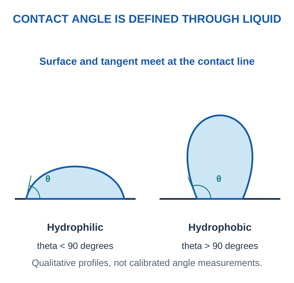
A water angle below 90° commonly describes hydrophilic behaviour and above 90° hydrophobic behaviour. Superhydrophobic surfaces are often associated with apparent angles above about 150° and low resistance to drop motion. A large static angle alone does not prove low adhesion.
Roughness and Wetting State
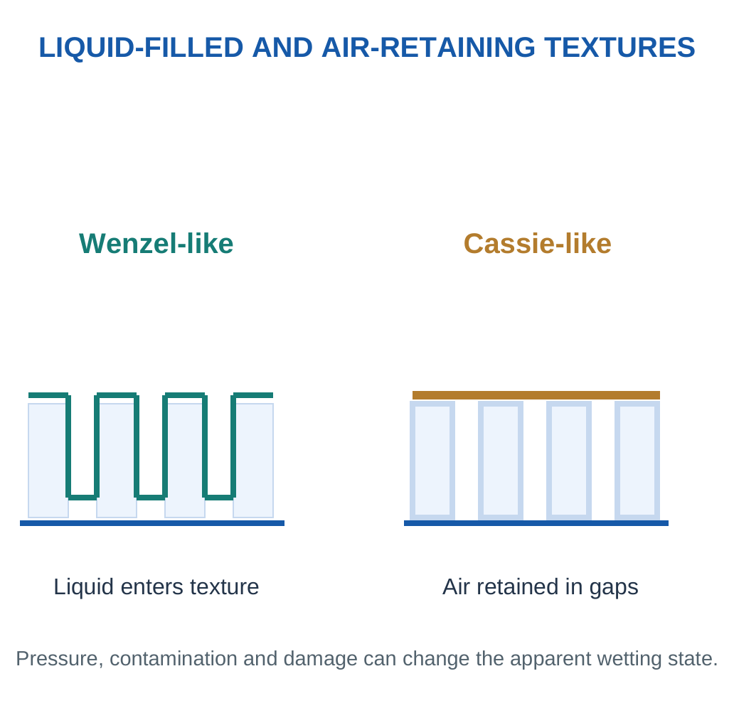
In a Wenzel-like state, liquid follows the surface texture more fully. In a Cassie-like state, air remains in some gaps. Pressure, vibration, wear or contamination can alter the state. A favourable initial state may therefore be unstable in service.
Key Point: What the Tangent Represents
The contact angle uses the tangent to the liquid interface at its contact with the solid, measured through the liquid. It is not an angle from the centre of the drop. An apparent angle on a rough surface can also depend on whether liquid enters the texture, so surface chemistry and wetting state both belong in the explanation.

Hysteresis and Mobility
Advancing and receding contact angles can differ because the contact line meets defects or chemical variation. This difference is contact-angle hysteresis. Sliding or roll-off tests provide distinct information about drop mobility.
Common Error: Hydrophobic does not automatically mean oil-repellent, chemically inert, permanently clean or self-cleaning. State the liquid and the required function.
Ideal Interfacial Balance
For an ideal smooth equilibrium surface, Young’s relation is:
γSG − γSL = γLG cos θ
The terms are solid-gas, solid-liquid and liquid-gas interfacial free energies. The equation explains why surface chemistry influences an equilibrium angle. Real rough, contaminated or chemically patchy surfaces can show apparent angles that require a more detailed model.
The angle is measured through the liquid. A larger angle means less spreading for that liquid under the comparison conditions; it does not measure the coating’s thickness or abrasion resistance.
Air Retention and Stability
An air-retaining texture can reduce solid-liquid contact, but pressure or impact can force liquid into gaps. A high initial angle can therefore coexist with poor robustness. Roughness can amplify wetting behaviour; it does not replace the role of surface chemistry.
Young’s Relation as a Balance of Interfaces
The solid-gas, solid-liquid and liquid-gas interfaces have associated free energies. At ideal equilibrium on a smooth chemically uniform surface, their horizontal balance gives Young’s relation. If replacing solid-gas contact by solid-liquid contact is relatively favourable, water can spread more readily and the angle is smaller under the model.
This does not require the solid to dissolve in the liquid. Wetting is an interfacial phenomenon. A water-repellent surface can still be attacked chemically under other conditions, and a hydrophilic surface can remain chemically stable in its intended service.
Advancing and Receding Measurements
When the contact line moves across new surface, an advancing angle can be observed. When it withdraws, a receding angle can be observed. Defects, roughness and chemical variation can pin the line, so the two values differ. The method, liquid volume and motion history should therefore accompany the values.
Water and Oil Are Different Tests
A surface described as hydrophobic concerns water. An oil can interact differently because its interfacial properties differ. Water beading does not prove oil repellence. A surface intended for oily contamination needs an appropriate additional test rather than reusing a water contact angle as evidence.
Explain the Boundary: Angle is local geometry at the contact line, hysteresis concerns history, and roll-off concerns drop motion under tilt. They are related but distinct observations.
Guided Derivation: Interpret an Interfacial-Energy Model
For an ideal smooth surface:
γSG − γSL = γLG cos θ
Rearranging:
cos θ = (γSG − γSL)/γLG
The numerator and denominator use the same interfacial-energy unit, so their ratio is dimensionless. The angle is measured through the liquid, consistent with the labelled droplet diagram.
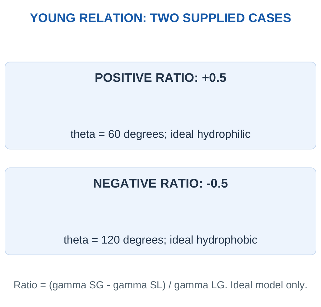
Teaching Case A
Let γSG − γSL = 0.036 N/m and γLG = 0.072 N/m.
cos θ = 0.036/0.072 = 0.5
θ = 60°
The result falls below 90° and describes hydrophilic behaviour within this supplied ideal model.
Teaching Case B
Change only the numerator to −0.036 N/m.
cos θ = −0.036/0.072 = −0.5
θ = 120°
The larger angle describes hydrophobic behaviour. The sign of the interfacial difference matters; using absolute values would lose the distinction.

What the Calculation Does and Does Not Establish
It explains an equilibrium angle for a stated smooth, uniform surface. It does not calculate contact-angle hysteresis, roll-off, abrasion resistance or chemical cleaning. A rough surface can have an apparent angle influenced by a wetting state and should not automatically be assigned the same ideal calculation.
If an input ratio lies outside −1 to +1, a simple inverse-cosine calculation does not produce a physical angle in this model. Check the inputs, definitions and whether the assumed equilibrium description is appropriate. Do not report a complex or arbitrarily clipped angle as an experimental result.
Connect the Derivation to a Surface Decision
A hydrophobic result can be useful for water management, but a real coating still needs drop mobility, coverage, adhesion and optical compatibility where relevant. A hydrophilic result can be useful for spreading a rinsing film. Neither category is universally superior. The required cleaning or device function determines what the angle contributes to the design.
Reasoning Check: A positive numerator gives a positive cosine and an angle below 90° in this model. A negative numerator gives an angle above 90°. The limit concerns the stated interfacial balance, not every possible real surface.
Worked Example 4.23: Contact-Angle Hysteresis
Problem: A surface has advancing angle 153° and receding angle 137°. Find hysteresis.
Model / Approach: Δθ = θadv − θrec; no roll-off-angle model is supplied.
Step 1: Identify the two dynamic-angle measurements.
Step 2: Subtract 153 − 137.
Step 3: Hysteresis is 16°.
Step 4: This describes contact-line history/pinning in the test. It does not directly give sliding angle or dirt-removal efficiency.
Answer: Hysteresis 16°.
Check and Interpretation: A static angle is not substituted for either dynamic measurement.
12. Testing Water-Repellent Surfaces
Compare coupons using the same liquid, drop volume, surface condition, temperature and method. Repeat across representative positions. Static angle, advancing/receding angles, drop mobility and abrasion resistance answer different questions.
Key Point: Match the Application Test
A transparent window needs optical clarity as well as water management. Strong roughness may help a wetting response while increasing haze. Compare all requirements rather than one attractive measurement.


If two surfaces both show large static angles but one releases drops at a much smaller tilt, the latter better supports mobile-drop cleaning under that test. A pinned drop can remain on an apparently hydrophobic surface.
Transparent-Window Requirements
A sensor window can require optical transmission, low haze, water management, adhesion and cleaning resistance. Strong roughness may improve one wetting response yet scatter too much light. Material selection must therefore use several requirements together.
A coating can fail through contamination, damaged texture, delamination or chemical ageing. Repeating the same initial contact-angle test without examining these causes may miss the mechanism.
Evidence Ladder: Appearance → calibrated wetting measurement → movement/cleaning test → durability under relevant conditions. Each stage supports a stronger and more specific claim.
Before-and-After Durability Comparisons
A meaningful durability test states what treatment the coating receives and how its function is measured afterwards. Abrasion, repeated washing, thermal cycling and environmental exposure stress different aspects of the material. A sample can retain a large static angle while its drop mobility worsens through damaged texture.
Controls for a Transparent Coupon
An untreated substrate provides a useful baseline. Compare optical transmission and haze as well as water behaviour. A coating that appears clear in one photograph may scatter enough light to impair a sensor or display in another geometry. Reflection, transmission and scattering are different optical routes.
Interpreting Spatial Variation
Measure more than one position if the coating can be uneven. A single excellent spot does not represent an entire window. Mapping or representative sampling can reveal poor coverage, edge effects or contamination. Report the observed spread rather than only the largest angle.
Decision Example
Coating A retains drop mobility after the specified cleaning test but coating B loses it. If optical and adhesion requirements are also met, A is better supported for that cleaning service. The conclusion is tied to the test; it does not establish that A resists every liquid, scratch or outdoor condition.
Worked Example 4.24: Choose a Mobile-Drop Candidate
Problem: A has static angle 156° and roll-off 6°; B has static angle 158° and roll-off 42°. Which better supports moving-drop cleaning?
Model / Approach: Comparable clean coupons and water tests; no oil or wear test supplied.
Step 1: Both show strong apparent water beading.
Step 2: A releases drops at much lower tilt.
Step 3: A better supports mobile-drop cleaning under this test.
Step 4: B illustrates why a high static angle alone is insufficient. Actual dirt removal and durability remain separate evaluations.
Answer: A is the initial moving-drop candidate.
Check and Interpretation: The 2° larger static angle of B does not override its greater pinning.
13. Self-Cleaning Surfaces: Distinct Mechanisms
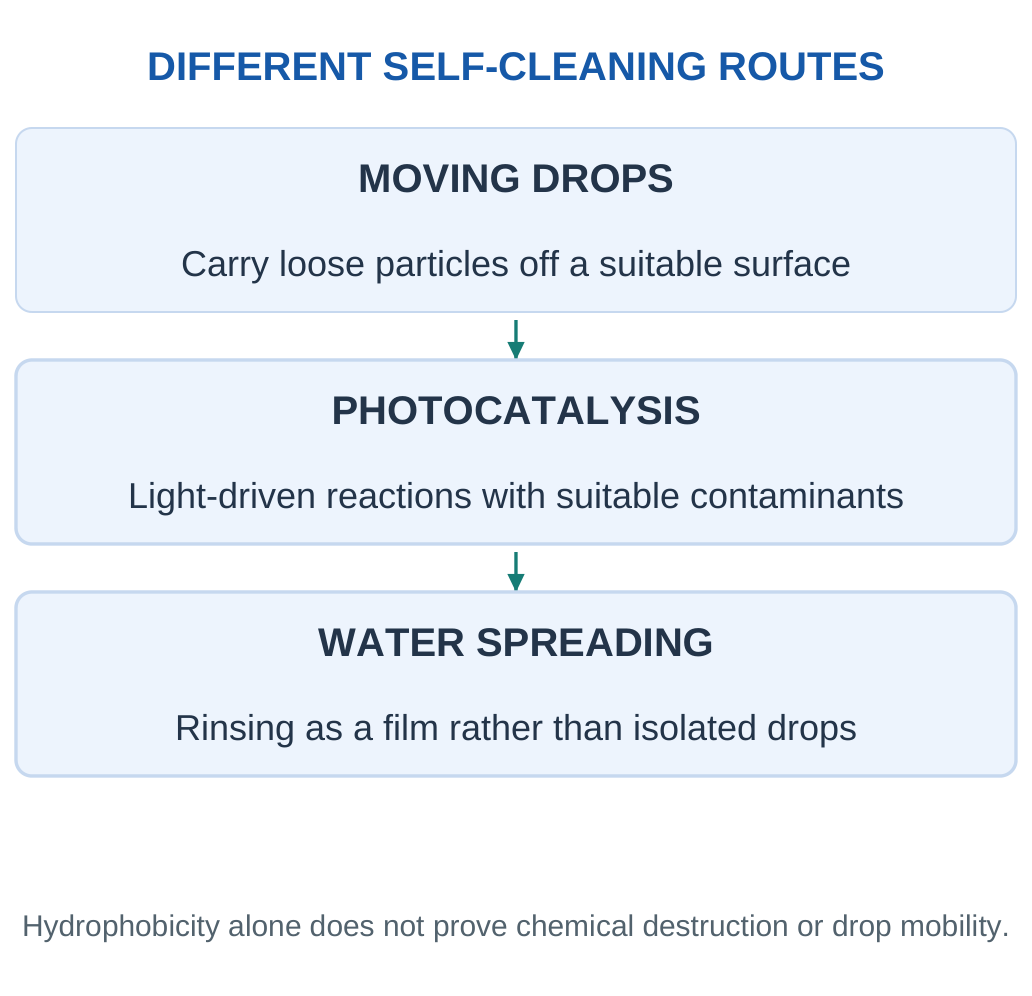
Self-cleaning reduces the need for external cleaning through a defined operating mechanism. Water-assisted particle removal and photocatalytic chemical transformation must be distinguished.

Mobile-Drop Route
On a suitable low-adhesion water-repellent surface, moving drops can collect loose particles. This lotus-effect concept depends on water availability, drop motion and dirt interactions. Sticky oily deposits or strongly attached particles can limit removal.
Photocatalytic Route
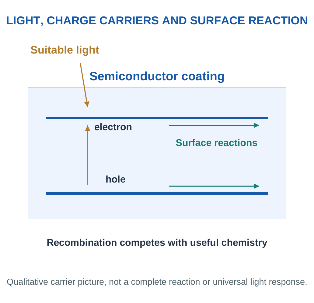
A suitable semiconductor coating, such as an appropriately designed TiO₂-based layer, absorbs light and generates charge carriers. Interfacial reactions can attack selected organic contaminants. Recombination competes with useful chemistry; illumination, oxygen, water, adsorption and coating condition matter.
A decrease in stain colour does not alone prove complete conversion to harmless final products. Inorganic dust may still require washing. A hydrophilic surface can spread water into a rinsing film without producing strongly beaded drops.
Key Point: Colour Loss Is Not Complete Mineralisation
A stain signal can fall through washing, desorption or transformation. Chemical-product evidence and a suitable balance are needed before claiming complete conversion to harmless products.


Comparison Framework: Mechanism → required conditions → type of contaminant → evidence → limitation. Hydrophobicity is a wetting property; photocatalysis changes chemistry.
A Labelled Photocatalytic Mechanism
For a suitable semiconductor, absorbed light can create an electron and a hole. They may reach the surface and participate in reactions, or recombine without performing the desired chemistry. Surface adsorption and transport determine which contaminants can interact with the active region.
Key Point: Test the Cleaning Route
A dark control can reveal adsorption or washing without illumination. An uncoated illuminated control helps separate coating effects from light alone. Product evidence is needed for a stronger chemical-transformation claim. Choose controls that answer the proposed mechanism, rather than treating every cleaner-looking coupon as proof of photocatalysis.
Key Point: Wetting and Cleaning Can Cooperate
A photocatalytic layer can transform suitable organics while water removes remaining material. A surface may also support water spreading rather than beading. Explain the role of each stage and the contaminant involved; there is no requirement that every self-cleaning surface be hydrophobic.

Controls Make a Cleaning Claim Stronger
Compare illuminated and dark conditions, coated and uncoated surfaces, and relevant washing conditions. These distinguish light effects, adsorption and simple physical removal. Measuring reaction products can support a chemical pathway. A stain becoming colourless is weaker evidence than a complete chemical balance.
A practical window also needs optical clarity and adhesion. A highly active powder is not automatically a durable transparent coating.
What Different Contaminants Require
Loose mineral particles can be physically removed by suitable moving water, while a bonded oily layer may resist that route. An appropriate photocatalytic surface can transform certain organics, yet remaining inorganic particles may still need rinsing. A complete self-cleaning design can therefore combine chemical and physical stages.
Apparent Cleaning Versus Chemical Fate
A material may become colourless without full mineralisation. It may also move from the surface into wash water. Both can reduce a visible stain while leaving products that need assessment. A strong claim follows the contaminants and products rather than only the appearance of the original coupon.
Light Access and Recombination
The coating must receive suitable light at the active region. Dirt, an unsuitable cover or a source lacking the needed wavelengths can limit activation. Generated carriers may recombine before useful reaction. These are mechanism-based reasons why the same coating can behave differently in two environments.
Explain a Mixed Result
If water rolls readily but an oily stain remains, the result does not automatically contradict hydrophobicity. The surface can repel water while the contaminant adheres strongly. If a photocatalytic test improves only under suitable illumination, the light-dependent mechanism needs appropriate controls and product evidence. A precise explanation names the route, contaminant and operating condition.
Application Workshop: Evaluate a Self-Cleaning Claim
A teaching study uses identical initial stain signals of 100 units. Four separate coupons receive different treatments. An uncoated dark coupon ends at 95, an uncoated illuminated coupon at 90, a coated dark coupon at 80 and a coated illuminated coupon at 40. Measurement conditions are matched; no chemical products are measured.
| Condition | Final Signal | Signal Decrease |
|---|---|---|
| Uncoated, dark | 95 | 5% |
| Uncoated, illuminated | 90 | 10% |
| Coated, dark | 80 | 20% |
| Coated, illuminated | 40 | 60% |
Step 1: Identify the Observation.
The coated illuminated sample has the largest reduction in the measured stain signal. That is the direct result, not yet a complete mechanistic explanation.
Step 2: Use the Controls.
The coated dark result shows that a change can occur without illumination. Adsorption or other non-light processes may contribute. The uncoated illuminated result shows that illumination can have an effect even without the coating. The combination must be interpreted against both controls.

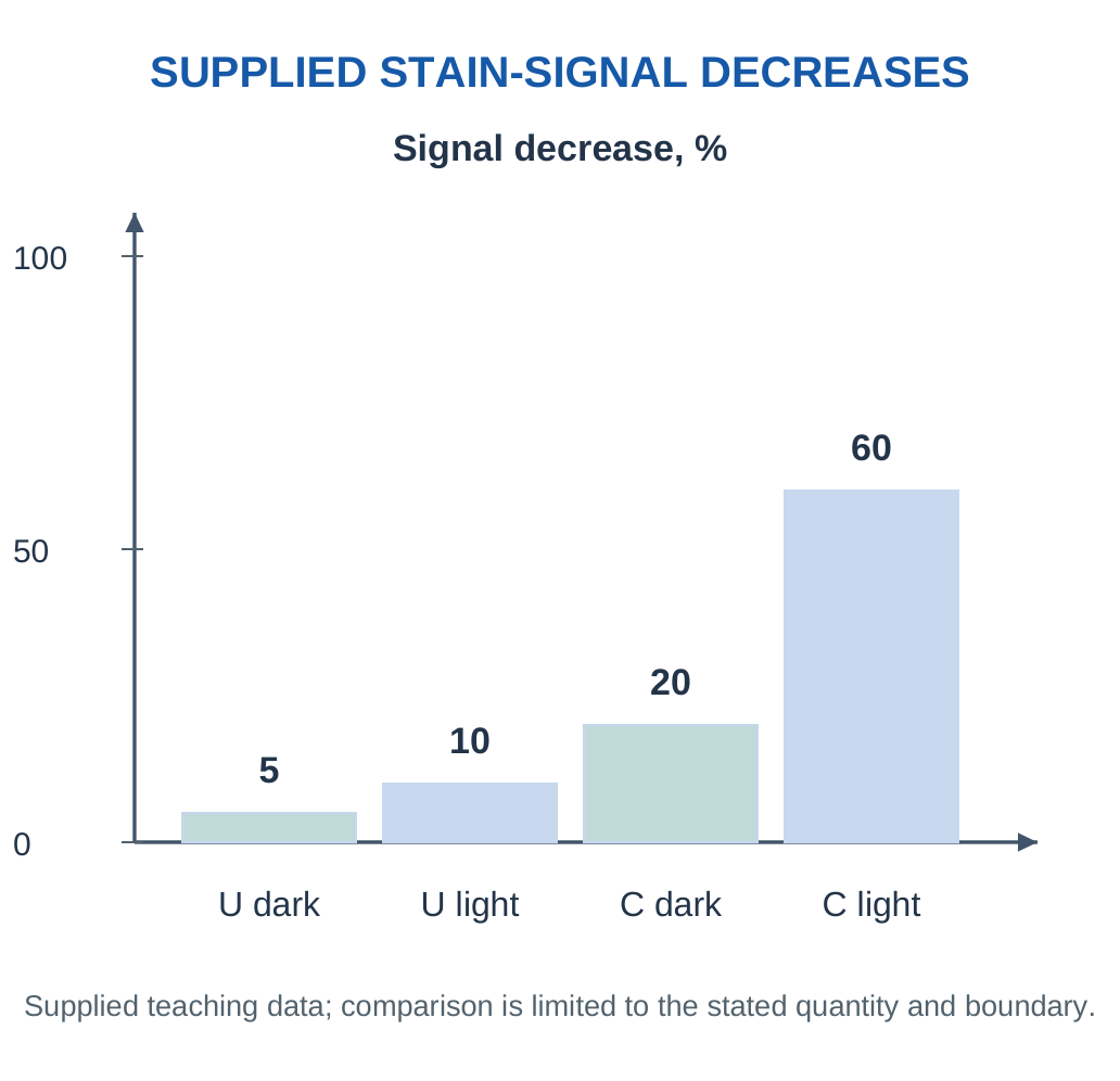
Step 3: Avoid an Unsupported Subtraction Claim.
Subtracting two percentages can describe a difference between observations, but it does not automatically isolate a pure photocatalytic fraction. Interactions and non-linear signal behaviour can matter.
Step 4: Strengthen the Claim.
Evaluate washing separately, examine whether the signal tracks actual contaminant mass and identify relevant products. For a practical window, also test optical clarity, adhesion and repeat use.
Workshop Conclusion: The data support an improved apparent stain-signal reduction for the coated illuminated condition. Complete degradation, harmless products and long-term self-cleaning remain stronger claims requiring further evidence.
Worked Example 4.25: Signal Reduction Versus Complete Degradation
Problem: Stain signal falls from 80 to 20 arbitrary units. Calculate reduction and interpret the limit.
Model / Approach: Comparable signal conditions; no chemical-product or carbon balance is supplied.
Step 1: Decrease = 80 − 20 = 60 units.
Step 2: Fractional decrease = 60/80 = 0.75.
Step 3: Signal reduction is 75%.
Step 4: Washing, desorption or chemical transformation could contribute. Signal loss alone does not prove complete mineralisation or harmless products.
Answer: 75% decrease in the stated signal.
Check and Interpretation: Optical disappearance and full chemical conversion are different claims.
14. Photochromic Materials
Photochromism is a reversible light-induced change between states with different absorption spectra. Activation and reversal can follow different photochemical or thermal pathways depending on the material.

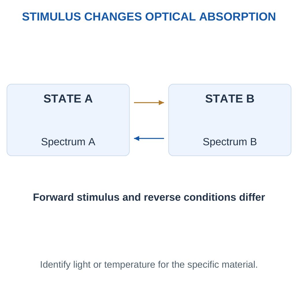
In an organic system, light can alter molecular arrangement or bonding, changing the electronic absorption. A polymer host influences mobility and stability. Inorganic photochromic systems may use other mechanisms, so identify the class rather than implying one reaction explains all materials.
Key Point: A Reversible Cue Can Fade
A photochromic state can recover while exposure history changes. A cumulative-dose interpretation needs a validated history-response model; tint alone is not a permanent exposure record.


Optical Quantities
Transmission:
T = I/I₀
Absorbance:
A = −log₁₀T
A lower T gives a higher A at the specified wavelength. A colour photograph cannot independently provide the spectrum, response time or ultraviolet dose.
Uses and Limitations
Lenses and light-responsive indicators use changes in transmission. Evaluate activation/recovery rate, cycling, temperature dependence and ageing. Filtering of activating wavelengths by a window can change response. A reversible tint needs calibration before it can be interpreted as a quantitative exposure reading.
Memory Aid: Photo = specified light trigger. Explain both forward change and recovery; naming only darkening leaves half the mechanism unstated.
Response, Recovery and Fatigue
Response time describes the change after a defined illumination begins. Recovery time describes return under specified reversal conditions. Both depend on the material, temperature, host and measurement definition. A single time without a defined fraction of change is ambiguous.
Repeated activation can gradually alter response amplitude or speed. Evaluate cycling under relevant conditions rather than assuming a reversible mechanism lasts indefinitely. Darkening and fading can also occur together, so steady tint may reflect competing rates.
Interpretation of an Indicator
A light-responsive layer may show that illumination affected the material. Inferring a cumulative exposure dose is stronger: it requires a relation between history and measured state, including any fading. A rapidly reversible lens should not be treated as a permanent exposure record.
Photochromism Is a State-Dependent Optical Property
Two states can have different electronic absorption because their molecular arrangement or solid-state environment differs. Illumination changes the population of states according to the material’s forward and reverse processes. A steady tint can therefore be a balance rather than complete conversion of every responsive unit.
Spectral Response and a Real Observer
The colour seen by eye depends on the illumination spectrum, wavelength-dependent transmission and viewing conditions. The same material can appear different under different lamps. A quantitative instrument uses a defined optical measurement instead of assigning concentration or exposure from a visual impression alone.
Lenses, Indicators and Records
A lens is intended to adjust transmission during changing light conditions. An exposure indicator may instead aim to retain or quantify a history. A reversible lens does not necessarily store that history. A device answer should state the information needed and then match the material’s response and recovery to it.
Useful Failure Questions
Has activation slowed, has the recovered baseline changed, or has the maximum contrast fallen? These observations suggest different changes. Repeat cycling, host stability and environmental access can influence performance. Calling all deterioration fading misses the difference between baseline drift, response amplitude and response speed.
Worked Example 4.26: Transmission and Absorbance
Problem: At one wavelength a lens changes from 80% to 25% transmission. Find absorbance in both states.
Model / Approach: A = −log₁₀T using fractional T and the same optical path.
Step 1: Initial T = 0.80 gives A₁ = 0.0969.
Step 2: Activated T = 0.25 gives A₂ = 0.6021.
Step 3: Absorbance increase ≈ 0.5052.
Step 4: The darkened state absorbs more at this wavelength, but the calculation does not supply its full visible spectrum or response time.
Answer: A₁ ≈ 0.097; A₂ ≈ 0.602.
Check and Interpretation: Using 80 instead of 0.80 inside the logarithm is incorrect.
15. Thermochromic Materials
Thermochromism is a temperature-dependent optical change. Molecular state, ordering or phase behaviour can change absorption or reflected colour. Leuco-dye and liquid-crystal systems are examples of different mechanisms, not one universal reaction.


Reversible and History-Recording Behaviour
A reversible material returns towards an earlier appearance on cooling through its response range. An irreversible label can retain evidence of a past event. Choose the response that matches the information required: current condition and past threshold crossing are different questions.
Heating and cooling thresholds can differ. This thermal hysteresis means that colour near the transition depends on recent history as well as current temperature. Ageing, viewing light and response time can also influence interpretation.
| Photochromic | Thermochromic |
|---|---|
| Triggered by specified light | Triggered by temperature |
| Recovery thermal or photochemical as specified | Heating/cooling paths may differ |
| Lens or light-exposure application | Temperature or thermal-history indication |
Thermochromic coatings can support packaging indicators and visual thermal displays. A visual change does not inherently generate electrical power; an electrical system needs a detector or a separate transduction route.
Quantitative Use: Specify the transition range, hysteresis, time response and calibration. A nominal activation temperature alone is not a complete thermometer specification.
Material Families and Use Conditions
In leuco-dye formulations, a temperature-dependent environment can change the coloured state. In liquid-crystal systems, ordering can change optical reflection. These examples emphasise that colour response can come from different microscopic mechanisms. The host, additives and encapsulation influence practical use.
Key Point: History Can Matter at One Temperature
A reversible thermochromic system with different heating/cooling thresholds can display different states at the same temperature. Name the path and the threshold before interpreting the colour.

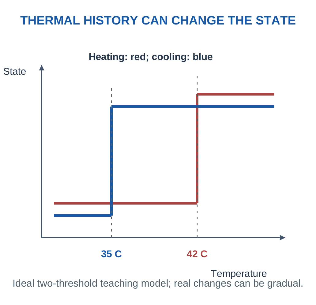
Choosing the Right Indicator
A reversible label can show current conditions within its response behaviour. An irreversible indicator is chosen when retaining a threshold event matters. An indicator cannot report a part of the temperature history that its chemistry does not store. Specify threshold tolerance, time at temperature, response delay and viewing conditions before interpreting a colour as an event record.
Temperature Response Is Not Always Instantaneous
A label senses its own material temperature, which can lag the temperature of the object or fluid of interest. Thermal contact, thickness and heat transfer influence that lag. A quick colour change in a thin coating does not guarantee the same response inside a thick package.
Hysteresis and Event Interpretation
With separate heating and cooling thresholds, the same temperature can correspond to different states. That behaviour can be useful for suppressing rapid switching, but it complicates an inverse temperature reading. A calibration should specify the direction of temperature change and the observation time.
Reversible Versus Irreversible Selection
Use a reversible response for a changing visual indication when its calibration is suitable. Use an appropriately designed retained change when a past threshold event must remain visible. The second choice still needs evidence of its threshold tolerance and time dependence; a permanent colour does not automatically identify the exact event duration.
Application Answer
For a thermal label, describe the responsive material, thermal contact, optical response, viewing method and intended inference. Include the environment and lifetime. A temperature cue for a package is different from an electrical temperature sensor, even if both support a smart monitoring system.
Worked Example 4.27: Interpret Thermal Hysteresis
Problem: A label switches hot on heating at 42°C and returns on cooling at 35°C. Find hysteresis and discuss its state at 38°C.
Model / Approach: Use the supplied ideal two-threshold history model.
Step 1: Threshold difference = 42 − 35 = 7°C.
Step 2: Heating from below 35°C to 38°C does not cross 42°C.
Step 3: Cooling from above 42°C to 38°C does not cross 35°C.
Step 4: The same 38°C can therefore show different states depending on history. Colour is not a unique thermometer within this interval.
Answer: Hysteresis 7°C; state at 38°C depends on prior history.
Check and Interpretation: A difference of 7°C equals a 7 K temperature interval.
16. Shape-Memory Polymers: A Programmed Cycle
A shape-memory polymer (SMP) retains a programmed temporary shape and recovers towards a stored permanent shape under a suitable stimulus. In a common thermal design, stable netpoints preserve the reference structure while switching domains become mobile across a transition.
The transition may involve glass transition or melting of a switching phase. Complete melting of the polymer is not required. Simply heating an ordinary plastic until it deforms does not demonstrate a programmed shape-memory cycle.

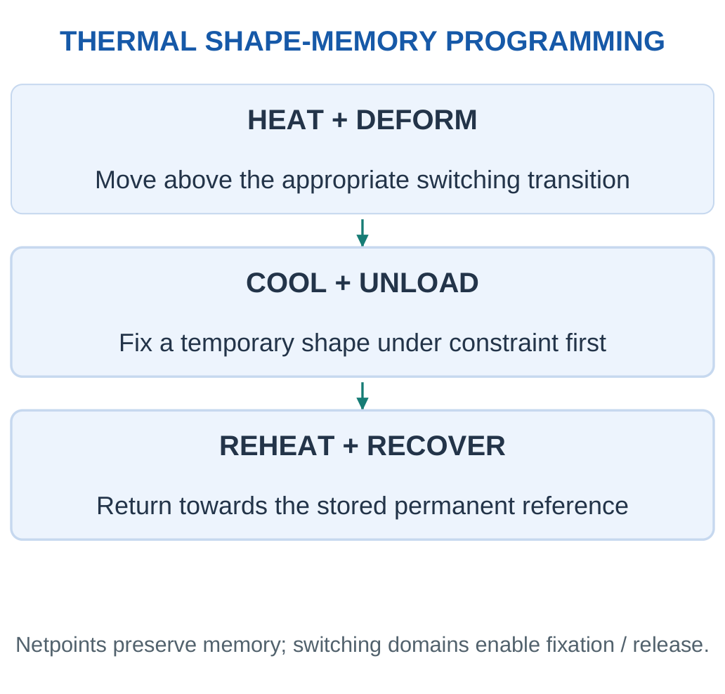
Steps of the Thermal Cycle
Step 1: Establish the permanent reference geometry through the network architecture or stable netpoints.
Step 2: Heat through the appropriate switching transition and deform within the supported range.
Step 3: Cool under constraint to restrict switching-domain motion; then unload to retain a temporary shape.
Step 4: Reheat appropriately so stored driving forces allow recovery towards the reference.
A common one-way SMP needs another programming step to produce a new temporary shape. Repeated automatic opening and closing with heating/cooling requires an appropriate two-way material/system, not merely the one-way effect.
Distinguish:
- Shape fixity describes retained temporary deformation after unloading.
- Shape recovery describes return towards the reference after triggering.
Where the Recovery Driving Force Comes From
During programming, the network is deformed while switching segments are mobile. Cooling constrains that motion and retains a non-equilibrium temporary configuration. When mobility returns, stored elastic driving forces can move the material towards the reference structure supported by stable netpoints. This explains the need for both memory-retaining and switching functions.
Switching Transition Versus Permanent Network
A glass transition can change segmental mobility without destroying all network connections. Melting of a suitable switching phase can play a related release role in another design. The permanent structure must remain sufficiently intact for recovery. Heating beyond a material’s supported range can instead damage it.
Why Programming Conditions Matter
Imposed strain, holding time, cooling under constraint and unloading conditions affect the retained shape. Recovery temperature, heating rate and load affect the return. Two reported recovery percentages are not fully comparable unless their test definitions and conditions match.

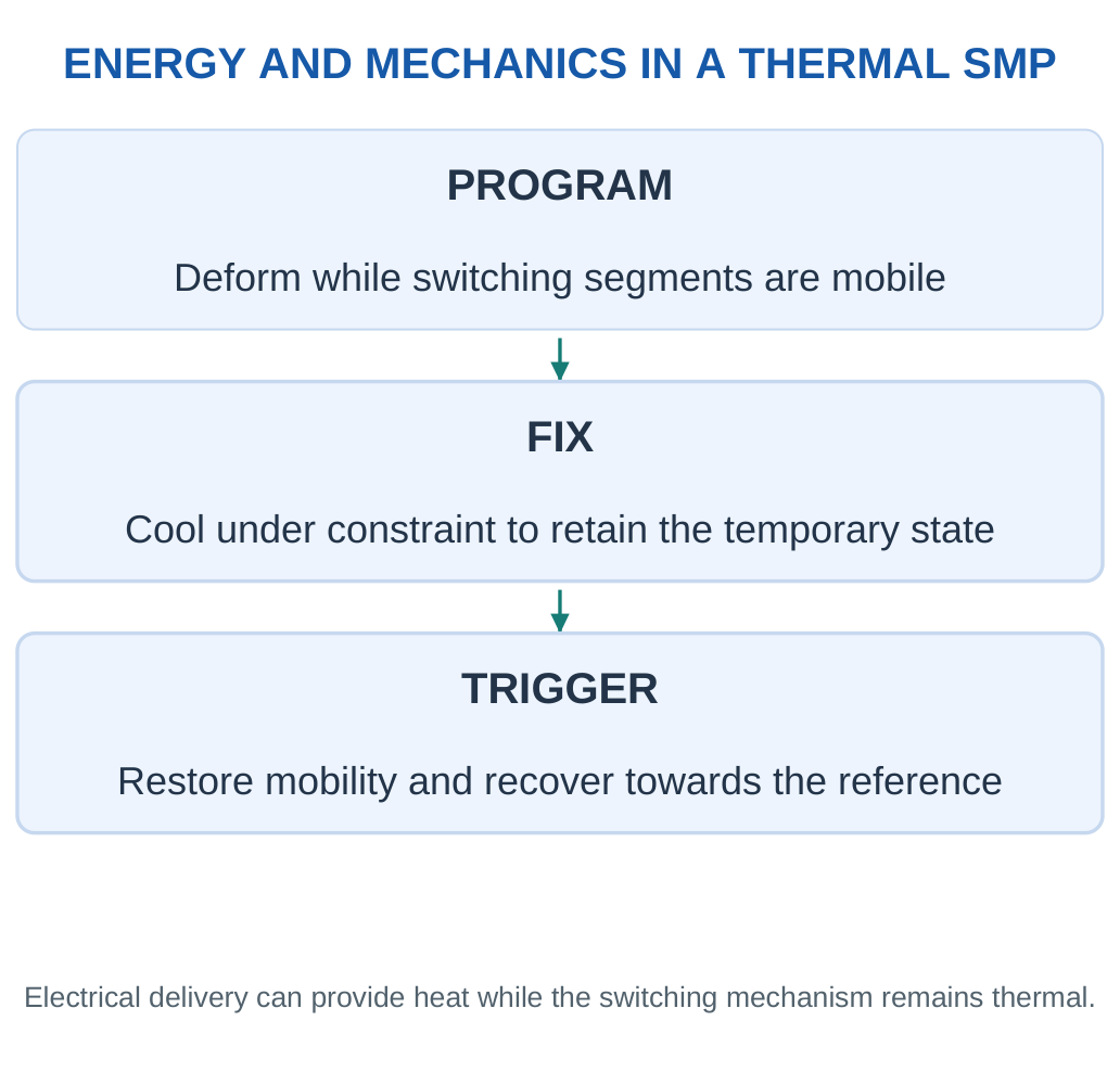
One-Way and Two-Way Behaviour
In a common one-way cycle, cooling after recovery does not recreate the temporary shape by itself. Another deformation/programming step is needed. Two-way behaviour requires a suitable material/system and operating arrangement. This distinction prevents the common mistake of drawing an endlessly repeating open-close cycle for any ordinary SMP.
Worked Example 4.28: Calculate Shape Fixity
Problem: Imposed strain is 40%; retained strain after unloading is 36%. Find fixity.
Model / Approach: Use Rf = εu/εm × 100% for this single cycle.
Step 1: Identify εm = 40% and εu = 36%.
Step 2: The ratio is 36/40 = 0.90.
Step 3: Fixity is 90%.
Step 4: Recovery has not been measured. The temporary shape can be well fixed even if later recovery is poor.
Answer: Shape fixity 90%.
Check and Interpretation: Both percentage strains can be replaced by matching decimal fractions.
17. Recovery, Actuation and Performance
In one simple single-cycle convention starting at zero residual strain:
- εm = imposed strain
- εu = retained strain after unloading
- εp = residual strain after recovery
Then:
Rf = εu/εm × 100%
Rr = (εm − εp)/εm × 100%
Cyclic definitions can differ, so use the convention supplied.
Key Point: Motion Is Not Force Capacity
A freely recovering strip can move substantially without producing a useful force against a load. Fixity, recovery, force, response time and fatigue are separate actuator requirements.


Delivering the Stimulus
Conductive filler can allow electrical current to provide Joule heating. Light-absorbing filler can convert irradiation into heat. When the polymer responds thermally, these are indirect thermal activation routes; identify both the energy source and the switching mechanism.
A Useful Actuator Needs More
Fixity and recovery percentages do not specify recovery force, time or fatigue resistance. A strip that recovers freely may behave differently against a load. Deployable structures, adaptive grips and responsive packaging need compatible transition ranges, geometry and reliability.
Important Limit: A large recovered strain is not unlimited load capacity. Match response, force, temperature and cycle life to the intended device.
Fixity, Recovery and Force Are Separate
High fixity means the programmed deformation remains after external constraint is removed. High recovery means the triggered material moves back towards its reference under the test definition. Recovery force describes interaction with an opposing load. A free strip can show impressive motion but little useful force.
Thermal Window and Service
The switching range must be compatible with storage and operation. A low transition can permit accidental recovery during service; a high transition may be unsuitable near a heat-sensitive component. Heating must reach the active region without damaging neighbouring layers.
Cycling can change residual strain and response time. Record the cycle convention, strain history and recovery condition. Avoid comparing a first-cycle percentage with a multi-cycle corrected definition as though the two formulas were identical.
Shape Fixity and Recovery in a Combined Test
A specimen can retain its temporary shape well after unloading yet recover only partly when triggered. Conversely, it can recover strongly from the deformation that remains while showing poor initial fixation. Report both properties with the strain convention rather than calling either one the shape-memory efficiency without definition.
Free Recovery and Constrained Recovery
Free recovery measures movement with little opposing constraint. A constrained test measures a force or stress response while motion is restricted. An actuator may need both adequate stroke and adequate force. A photograph of a moving strip supplies neither complete load capability nor fatigue data.
Electrical Triggering and Energy Accounting
When current provides heat, the circuit’s electrical energy is not all converted into useful recovery work. Some raises the material temperature and some is lost to the surroundings. A device can be electrically triggered while the polymer’s switching mechanism remains thermal. These descriptions answer different questions.
Design Comparison
For a deployable component, consider temporary-shape storage, accidental trigger conditions, recovery completeness and available force. For a repeated grip, consider programming/reset needs and fatigue. A material that suits a single deployment may be unsuitable for rapid repeated motion. Match the cycle to the service rather than treating every shape change as the same actuator function.
Application Workshop: Choose a Deployment Material
A compact component must retain a temporary folded form during storage and later recover under a defined thermal trigger.
| Material | Fixity | Recovery | Recovery Force |
|---|---|---|---|
| A | 98% | 70% | Adequate |
| B | 90% | 95% | Adequate |
| C | 95% | 96% | Inadequate |
Required fixity is at least 90% and required recovery at least 90%, with adequate force.
Step 1: Apply All Requirements.
A retains the temporary shape well but fails recovery. B meets both percentage thresholds and the force requirement. C meets both percentage thresholds but fails force. B alone passes the supplied initial screen.
Step 2: Interpret the Percentages.
Fixity concerns retention after unloading, while recovery concerns the triggered return. Neither describes the force available against a load. A large visible motion in a free specimen does not establish adequate deployment force.
Step 3: Check the Thermal Window.
A screened candidate must still retain its temporary form through intended storage and service before the trigger. Accidental exposure near the switching range can change its state. The trigger must also be compatible with surrounding parts.
Step 4: Evaluate the Complete Cycle.
Assess response time, repeated programming if needed, residual strain and fatigue. A single-use deployment and a repeatedly resetting actuator have different requirements. The supplied screen does not establish either lifetime automatically.
Workshop Conclusion: B is the supported initial candidate, not a universally best SMP. The selection follows the required cycle, force, transition range and reliability, rather than the largest isolated percentage.
Guided Case: Energy Input Is Not Mechanical Output
A small thermally activated element receives 6 W electrical power for 20 s. Its completed motion lifts a supplied 0.20 kg load through 0.05 m. Use g = 9.81 m/s². Assume the motion is quasi-static for the simple load-work calculation, and treat the stated electrical input as the complete included input for this comparison.
Step 1: Input Energy.
Electrical energy = Pt = 6 × 20 = 120 J
This describes delivered circuit energy; it is not the material temperature or the recovery strain.
Step 2: Useful Load Work.
Increase in gravitational potential energy:
mgh = 0.20 × 9.81 × 0.05 = 0.0981 J
This is one defined useful mechanical output, not necessarily every form of mechanical energy in the assembly.
Step 3: Compare the Boundary.
Useful-work/input ratio = 0.0981/120 = 0.0008175
As a percentage: 0.0818% approximately
Much of a thermal trigger’s input can heat the material or surroundings rather than appear as useful load work. The exact partition would require further thermal and mechanical information.

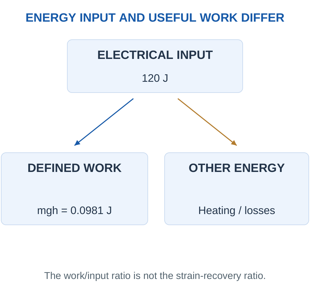
Step 4: Avoid a Misleading Conclusion.
This small supplied example does not establish the efficiency of every SMP actuator. Its value is to demonstrate that a 90% recovery ratio can coexist with a much smaller useful-work/input ratio because they use entirely different quantities and denominators.
What a Complete Actuator Specification Needs
State stroke, load, force or stress, trigger conditions, response time and cycle requirements. A deployment task may tolerate a slow trigger but require reliable storage. A repeated mechanism may need a practical reset and programming route. The appropriate design follows those requirements.
Numerical Check: Watts × seconds gives joules. Kilograms × m/s² × metres also gives joules. Only after both quantities share an energy unit is their ratio meaningful.
Worked Example 4.29: Calculate Shape Recovery
Problem: A zero-residual starting cycle is programmed to 50% strain and ends at 5% residual strain. Find Rr.
Model / Approach: Use Rr = (εm − εp)/εm × 100%, the stated convention.
Step 1: Programmed strain is 50%.
Step 2: Removed strain in this definition is 50 − 5 = 45 percentage points.
Step 3: Rr = 45/50 × 100 = 90%.
Step 4: The remaining 5% strain means incomplete recovery; it does not imply 95% recovery because the denominator is programmed strain.
Answer: Recovery 90% under the stated definition.
Check and Interpretation: Do not mix this definition with a different cyclic convention.
Worked Example 4.30: Electrical Activation Energy
Problem: A heater operates at 12 V and 0.5 A for 20 s. Find electrical power and energy.
Model / Approach: Constant voltage/current; useful heating fraction and losses are not supplied.
Step 1: Power = VI = 6 W.
Step 2: Energy = Pt = 6 × 20 = 120 J.
Step 3: This is electrical energy delivered to the circuit.
Step 4: Temperature rise and recovery time need heat capacity, geometry, losses and transition information. Joule heating can still trigger a thermal SMP mechanism.
Answer: 6 W and 120 J.
Check and Interpretation: W × s gives joules, not a temperature.
Worked Example 4.31: Read a Complete Single-Cycle Strain Ledger
Problem: An SMP starts with zero residual strain, is programmed to 60%, retains 54% after unloading and ends at 6% after recovery. Find fixity and recovery under the supplied definitions.
Model / Approach:
Rf = εu/εm × 100%
Rr = (εm − εp)/εm × 100%
Do not substitute a different cyclic convention.
Step 1: Fixity compares retained temporary strain with imposed strain:
Rf = 54/60 × 100 = 90%
This describes what remains after unloading.
Step 2: Recovery compares programmed strain removed by the final state:
Rr = (60 − 6)/60 × 100 = 90%
This uses imposed strain as the stated denominator.
Step 3: The equal percentages are coincidental to these values. Fixity and recovery remain separate stages; one cannot be inferred from the other in a different dataset.
Step 4: The ledger does not state recovery time, force against a load or stability over repeated cycles. Those would need additional defined measurements for an actuator decision.
Answer: Fixity 90%; recovery 90% under the stated single-cycle convention.
Check and Interpretation: A residual 6% does not imply 94% recovery when the imposed strain is only 60%.
18. Flexible Electronics and Bending Strain
Flexible electronics retain function while bending or conforming. A polymer support, compliant conductors, functional films and small rigid islands can be combined. Flexibility and stretchability differ: curvature change is not the same as in-plane extension.
Key Point: A Bend Test Is Scoped
Radius, cycle count, direction and measurement conditions define the result. Passing one bend radius does not establish resistance to every wearable motion or in-plane stretching.


For a thin homogeneous film of thickness t bent to radius R, an outer-surface estimate is:
|ε| ≈ t/(2R)
It assumes t is much smaller than R and the neutral plane is near the middle. Use the same length unit for both quantities.

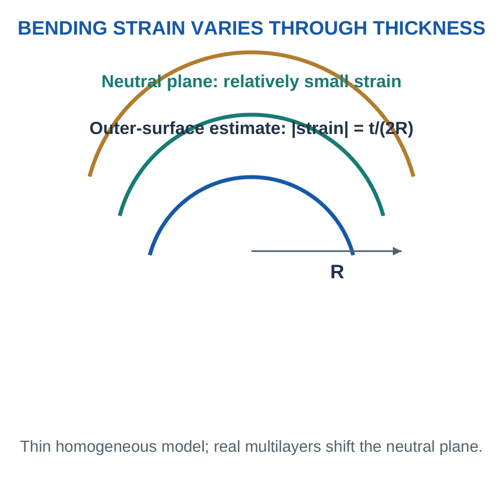
Reliability Tests
Repeated bending can cause cracks, delamination, contact failure and network changes. State bend radius, cycles, direction and measurement conditions. Moisture and thermal cycling may act together with mechanical stress.
Relative resistance change ΔR/R₀ can track electrical behaviour, but its acceptability depends on circuit tolerance. A single successful bend is not a lifetime test.
Design Choices: Reduce thickness, increase bend radius or place a brittle active layer near the neutral plane. Check insulation and support requirements while applying these strategies.
Layer Architecture
A flexible stack may contain a substrate, conductor, active layer and encapsulation. A thin brittle layer near a neutral plane can experience less bending strain, while compliant interconnect geometry can accommodate motion between rigid islands.

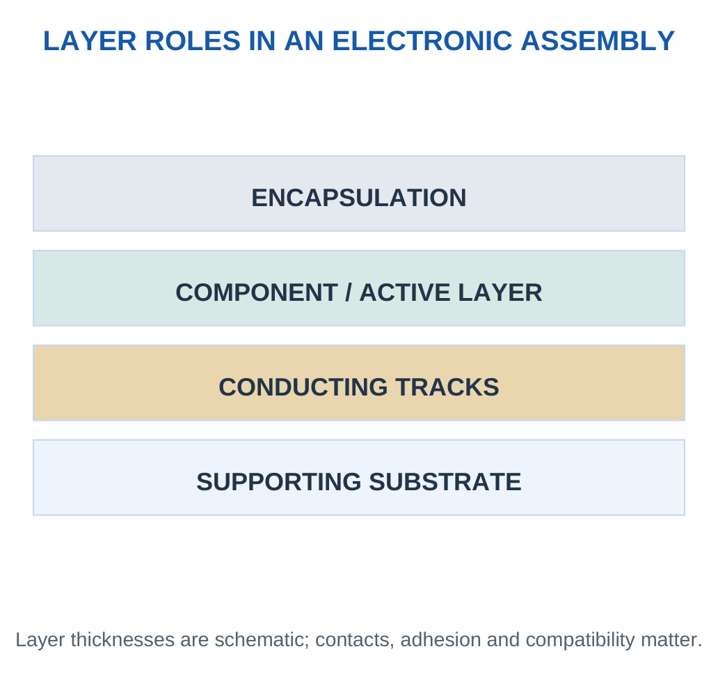
Bending Versus Stretching
A sheet bent into a cylinder can change curvature without much extension at its neutral plane. Stretching instead changes in-plane distance. Serpentine tracks can partly unfold geometrically, but they still need a supported strain range. Passing a bend test does not prove a stretchable device.
Report Reliability Honestly
State initial and final resistance, bend radius, cycles and conditions. A stable track at one radius can fail at a tighter radius. Compare devices under matched tests and interpret electrical changes against circuit requirements.
Strain Through a Layer Stack
In simple bending, fibres farther from the neutral plane experience larger extension or compression. A thin brittle layer near that plane can therefore experience less strain than a similar layer on the outer surface. Real stacks differ in thickness and stiffness, so the neutral plane is not always the geometric mid-plane.
Rigid Islands and Compliant Interconnects
A small rigid chip can sit on an island while surrounding interconnects accommodate relative motion. Serpentine paths can change shape geometrically, reducing the direct extension imposed on a straight conductor under some conditions. The path still has a limited range and can fail at contacts or tight curves.
Electrical Function During Motion
Continuity after unloading does not necessarily establish function while bent. Some contacts open intermittently, and resistance can change with position. A useful test observes the relevant output during the intended motion and after repeated cycles. The timing of measurement should be stated.
Interpret the Failure Location
A conductor crack, poor island connection and substrate delamination can all interrupt a signal. Visual inspection and electrical localisation help distinguish them. Improving the wrong layer may not improve the device. This is why flexible-electronics answers should include the assembled stack and contact route rather than only the name of a flexible material.
Worked Example 4.32: Estimate Bending Strain
Problem: A 100 μm homogeneous film bends to radius 10 mm. Find outer strain.
Model / Approach: ε ≈ t/(2R), mid-thickness neutral plane and thin-film assumption.
Step 1: Convert thickness to 0.100 mm.
Step 2: Use matched units:
ε = 0.100/(2 × 10)
Step 3: ε = 0.005 = 0.5%.
Step 4: The estimate does not establish fatigue life or the neutral plane of a real multilayer stack.
Answer: Outer-surface strain approximately 0.5%.
Check and Interpretation: Thinner film or larger radius reduces this estimate.
Worked Example 4.33: Find a Minimum Radius
Problem: A 60 μm film must keep estimated strain ≤0.3%. Find minimum radius.
Model / Approach: Use the same homogeneous model and decimal strain.
Step 1: t = 0.060 mm; εmax = 0.003.
Step 2: R ≥ t/(2εmax).
Step 3: R ≥ 0.060/0.006 = 10 mm.
Step 4: A tighter bend exceeds the model limit. Add appropriate material and cycling evidence for a real device.
Answer: Minimum model radius 10 mm.
Check and Interpretation: Substitution returns ε = 0.003.
19. Smart Devices Combine Complementary Layers
A wearable patch needs support, conduction, response, insulation, protection and readout. No single nanomaterial automatically provides every function.
Key Point: Communication Does Not Add Selectivity
Wireless electronics can transmit a measured value, but they do not establish what caused the material response. Recognition, transduction, calibration and communication remain different functions.

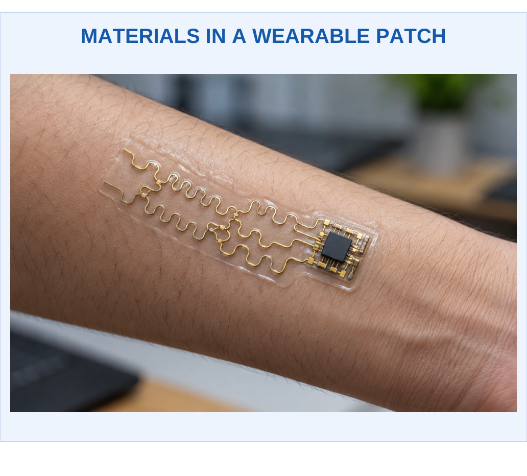
Flexible Strain Patch
A CNT network can provide a strain-dependent resistance, while conducting tracks route the signal. A compliant support follows a surface and an insulating layer controls electrical access. Calibration translates a defined signal into strain; temperature and humidity need relevant controls.
Smart Optical Window
A transparent electrode supports electrical access, a photochromic layer can change transmission and an outer coating can manage wetting. Their roles are distinct. Added layers can introduce haze, stiffness or adhesion problems, so combined performance needs testing.
Responsive Package
A thermochromic region can report a thermal condition and a shape-memory element can enable a triggered geometry change. The optical indication and mechanical output communicate different information.

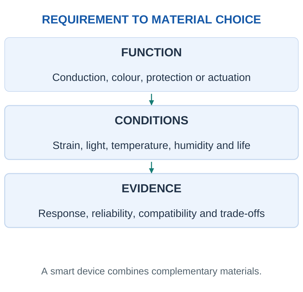
Long-Answer Pattern: Requirement → material choice → mechanism → labelled layer diagram → measured output → relevant limitation.
A Material-Selection Example
For a transparent wearable electrode, evaluate electrical loss, optical transmission, flexibility, adhesion and compatibility with skin-facing packaging. A film with the lowest resistance may be too opaque. A highly transparent network may drift under humidity. A stable encapsulation may obstruct a chemical sensing surface.
Separate Signal and Communication
A responsive material creates or changes a measurable quantity. Electronics convert that quantity into a reported result; wireless communication transmits it. Sending a resistance value does not make the material selective for one chemical or remove the need for calibration.
Design Review
Write the required input range, output, environment and lifetime first. Select materials with evidence for those conditions, then test the combined device. This prevents a list of attractive isolated properties from being mistaken for a complete engineering design.
Case Study: A Combined Motion and Temperature Patch
A patch can contain a resistance-based strain element and a separate temperature-responsive element. The strain output may also depend on temperature, so the design uses the second measurement to support a justified correction or interpretation. The correction must be validated; merely adding another sensor does not automatically remove interference.
The substrate supports motion, interconnects route signals and encapsulation protects selected regions. The active surface must remain accessible if the intended input requires contact. A waterproof barrier useful for one sensor can obstruct another sensing chemistry.
Case Study: A Responsive Window
A transparent electrode, optical-response layer and outer wetting layer can be combined. The electrode must carry charge, the optical layer must provide the intended spectrum and the outer layer must preserve clarity and surface function. Deposition of one layer can damage another, while additional interfaces can cause delamination or reflection.
System Evidence
Test each material function, then the combined assembly. Check whether one activation condition changes an unintended output. A real smart system is judged by a useful calibrated response under service conditions, not by adding the words nano, flexible and intelligent to a material list.
Integrated Reasoning: The device requirement chooses the material; processing creates its structure; interfaces connect it to the system; measurements establish the actual output.
Application Workshop: Flexible-Patch Design Review
A patch must track forearm bending. Its sensing network provides a resistance response, a small rigid chip performs readout and a flexible substrate supports both. The prototype works when flat but produces intermittent readings during motion. A design review should locate the failure before replacing the active material.
Step 1: Separate Sensing from Continuity.
Measure whether the active network gives a reproducible response under controlled strain. Then inspect the signal path through tracks, island contacts and connectors. An intermittent connection can imitate a very large sensor change.
Step 2: Separate Bending from Stretching.
Forearm motion can impose curvature and extension in different regions. A film that tolerates bending around a cylinder may not tolerate in-plane extension. The test should represent the actual local deformation.
Step 3: Assess the Stack.
The active layer’s distance from the neutral plane influences bending strain. Layer stiffness, thickness and bonding determine the actual distribution. Reducing total thickness or changing placement can help, but must retain insulation and mechanical support.

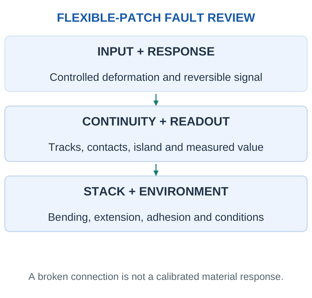
Step 4: Check Environmental Effects.
Temperature and humidity can change the network baseline or adhesion. A reference or compensation channel is useful only when its correction relation is supported by relevant tests.
Step 5: Retest the Assembled Device.
Verify output during motion and after repeated cycles at stated conditions. Passing isolated material tests is necessary evidence, but system interactions can still change the final result.
Workshop Conclusion: A systematic review follows input → material response → connections → readout. It preserves the distinction between a useful sensing signal and damage or communication failure.
Worked Example 4.34: Select by Two Specifications
Problem: A design needs transmission ≥85% and Rₛ ≤60 Ω/sq.
| Candidate | Transmission | Sheet Resistance |
|---|---|---|
| A | 90% | 80 Ω/sq |
| B | 86% | 55 Ω/sq |
| C | 80% | 30 Ω/sq |
Model / Approach: Apply both initial limits before ranking other properties.
Step 1: A passes transmission but fails resistance.
Step 2: B passes both limits.
Step 3: C passes resistance but fails transmission.
Step 4: B is the only initial candidate. Contacts, adhesion, bend stability and ageing still require assessment.
Answer: B alone meets both supplied specifications.
Check and Interpretation: Choosing only the lowest resistance would incorrectly favour C.
Worked Example 4.35: Read a Bending Test
Problem: Resistance rises from 80 to 92 Ω after 1000 specified bend cycles. Find relative change.
Model / Approach: Same measurement conditions; no general lifetime law is implied.
Step 1: ΔR = 92 − 80 = 12 Ω.
Step 2: Relative change = 12/80 = 0.15.
Step 3: Resistance rises by 15%.
Step 4: Whether this passes depends on circuit tolerance. Increased resistance can be degradation rather than improved performance.
Answer: 15% resistance increase.
Check and Interpretation: Use initial resistance as denominator, not the final reading.
Worked Example 4.36: A Complete Two-Requirement Reliability Decision
Problem: A flexible electrode must have R ≤150 Ω initially and ≤20% resistance increase after its stated bend test.
- A gives 120→150 Ω.
- B gives 140→154 Ω.
- C gives 170→175 Ω.
Choose a candidate.
Model / Approach: Apply both supplied requirements. The test is comparable across candidates; no optical or skin-compatibility evidence is supplied.
Step 1: A passes initial resistance but changes by:
(150 − 120)/120 = 25%
This exceeds the 20% change limit. A fails the combined requirement.
Step 2: B passes initial resistance and changes by:
(154 − 140)/140 = 10%
This satisfies the stated change limit. Its final resistance is not compared with a separate final limit unless one is specified.
Step 3: C changes by about 2.94%, but its initial 170 Ω exceeds 150 Ω. A small fractional change does not compensate for failing the initial specification.
Step 4: B is the initial candidate on these two criteria. Optical transmission, adhesion, environmental stability and the actual circuit still need appropriate evaluation before final device selection.
Answer: B alone meets both stated criteria.
Check and Interpretation: Read each limit exactly: an initial-resistance limit and a change limit are not the same as a final-resistance limit.
20. Formula Guide and Selection Summary
| Relation | Scope |
|---|---|
| 1 nm = 10⁻⁹ m | Unit conversion |
| A/V = 6/d for spheres | Exposed smooth geometry |
| R = RₛL/W | Uniform rectangular film |
| GF = (ΔR/R₀)/ε | Supplied linear strain response |
| E(eV) ≈ 1240/λ(nm) | Photon-energy conversion |
| Φ = emitted/absorbed photons | Photoluminescence quantum yield |
| T = I/I₀; A = −log₁₀T | Fractional transmission and absorbance |
| ε ≈ t/(2R) | Thin homogeneous bend estimate |
| Rf = εu/εm × 100% | Stated single-cycle fixity |
| Rr = (εm − εp)/εm × 100% | Stated single-cycle recovery |
How to Avoid Numerical Errors
A percentage strain must become a fraction in the gauge-factor equation. A 40% transmission becomes T = 0.40 inside the logarithm. Nanometres and millimetres must be matched before a geometric ratio. Photon energy cannot give dot diameter without an additional material model.
Select and Verify
- For a conductor, assess contacts and continuity.
- For a display material, assess spectrum, efficiency and ageing.
- For a wetting coating, assess angle, mobility, adhesion and wear.
- For a chromic layer, assess response and recovery.
- For an SMP, assess fixity, recovery, force and cycling.

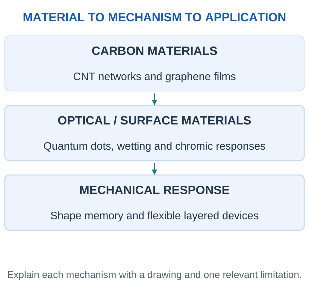
Nanomaterial form affects exposure: a filler immobilised in a sound polymer differs from a loose powder. Composition, structure and operating conditions should guide responsible processing and end-of-life handling.
21. Short-Answer Revision
1. Why Can Nanoscale Behaviour Differ from Bulk?
Interfaces, electronic confinement and geometry can become more influential. State which mechanism applies rather than assuming all nanoparticles behave alike.
2. What Is Percolation?
It is development of a connected conducting path across a material. Filler shape, dispersion and junctions influence its threshold.
3. Are All CNTs Metallic?
No. Single-walled CNT electronic behaviour depends on structure, including chirality and diameter. Networks add contact and junction effects.
4. Why Is Graphene Not a Universal Logic-Switch Replacement?
Ideal monolayer graphene lacks a conventional band gap. Good conduction does not automatically provide the low off-state current needed in a digital switch.
5. What Does Sheet Resistance Mean?
It normalises resistance for a uniform thin film. A rectangular film has R = RₛL/W under the simple model, with L/W counting squares.
6. Why Can Smaller Quantum Dots Emit Higher-Energy Photons?
Stronger confinement can increase the effective gap within a comparable semiconductor family. Composition and surface states also affect emission.
7. Is Quantum Yield Electrical Efficiency?
No. Photoluminescence quantum yield counts emitted photons per absorbed photon; electrical efficiency includes additional conversion and energy terms.
8. Is a Hydrophobic Surface Necessarily Self-Cleaning?
No. Drops may be pinned and dirt may adhere strongly. Mobile-drop cleaning needs suitable mobility and dirt interactions.
9. Why Measure Advancing and Receding Angles?
Their difference describes hysteresis and contact-line pinning, adding information beyond one static angle.
10. How Can a Hydrophilic Surface Aid Cleaning?
Water can spread into a washing film. A suitable photocatalytic layer may also transform certain organic contaminants.
11. What Differentiates Photochromism and Thermochromism?
Photochromism uses a specified light trigger, while thermochromism responds to temperature. Reversal and history effects depend on the system.
12. Why Distinguish Reversible and Irreversible Indicators?
A reversible state can report a current condition; a retained irreversible change may record a past event. They answer different questions.
13. What Stores Permanent Shape in an SMP?
Stable netpoints preserve the reference structure while switching domains fix and release temporary deformation.
14. Are Fixity and Recovery Identical?
No. Fixity measures retained temporary shape after unloading; recovery measures return towards a reference after triggering.
15. Does Flexible Mean Stretchable?
No. Bending changes curvature while stretching changes in-plane length. A film can tolerate one and fail under the other.
16. Why Place a Brittle Layer Near a Neutral Plane?
Bending strain is smaller there. The actual position in a multilayer depends on thickness and stiffness.
17. Why Must a Smart Device Use Several Materials?
Support, conduction, sensing and protection need different properties. Compatibility and combined reliability determine performance.
18. What Can an Appearance Photograph Prove?
It can show macroscopic form and assembly context. Nanoscale identity, purity, layer count and calibrated performance require other evidence.
22. Complete Examination Answers
1. Nanoscale Size and Material Behaviour
Nanotechnology engineers matter at roughly 1–100 nm to use behaviour associated with that scale. Subdivision increases exposed surface area per volume; for spheres, A/V = 6/d. This can affect adsorption and interfacial reactions.
Suitable semiconductor structures can also confine carriers, changing allowed states and optical response. Nanoscale geometry further changes how conducting paths and interfaces form. CNT networks, graphene films and quantum-dot emitters illustrate different mechanisms.
Composition, defects, aggregation and surface chemistry determine whether a size effect benefits a device. Reduced size alone is therefore not a sufficient explanation of improved performance.
2. CNTs and Graphene in Smart Electronics
CNTs and graphene contain related sp²-bonded carbon networks. A CNT has a tubular wall and high aspect ratio, whereas graphene is a sheet-like layer.
CNT networks can provide conducting or strain-sensitive paths in composites; graphene-containing films can support transparent electrodes and responsive interfaces. Tube structure influences CNT electronic behaviour, while tube junctions influence network resistance.
Graphene film continuity, defects and contacts control practical transport, and ideal monolayer graphene lacks a conventional band gap. The appropriate choice depends on the required geometry, electrical response, optical transmission and processing compatibility.
3. Quantum-Dot Colour Conversion
Quantum dots can confine carriers and exhibit size-sensitive optical behaviour. In a colour-conversion display, a suitable source excites the dots, part of the incident light is absorbed and selected emission is directed through the optical stack.
The photon relation E = hc/λ connects shorter wavelength with higher energy. Absorption fraction, photoluminescence quantum yield and extraction describe different stages and use different denominators.
Packaging helps control moisture, oxygen and heat-related degradation. Material quantum yield is consequently only one part of display performance; it is not the complete electrical-to-optical efficiency.
4. Two Self-Cleaning Mechanisms
A low-adhesion water-repellent surface can allow moving drops to collect loose particles. Its performance depends on surface chemistry, texture, hysteresis, water availability and dirt interactions.
A photocatalytic coating instead absorbs suitable light and uses photogenerated carriers for reactions with selected contaminants. Hydrophilic water spreading can additionally help rinse material away.
Water repellence is a wetting property, while photocatalysis changes chemistry. Abrasion, contamination and unsuitable operating conditions can limit either route. A lower stain-colour signal alone does not prove complete mineralisation or harmless final products.
5. Photochromic and Thermochromic Responses
Photochromic materials reversibly change optical absorption under specified illumination. Their recovery can be thermal or photochemical, depending on the system.
Thermochromic materials change optical appearance with temperature through suitable molecular, ordering or phase behaviour. A reversible label can indicate a current condition, while a suitable irreversible response can retain a past event.
Lenses and temperature indicators illustrate the applications. Response time, hysteresis, cycling and ageing influence interpretation. A visual change becomes a quantitative reading only when its relation to the input is calibrated under relevant conditions.
6. Thermal Shape-Memory Cycle
A common thermal SMP combines stable netpoints with switching domains. The netpoints preserve a permanent reference structure.
Heating through the appropriate switching transition permits deformation; cooling under constraint fixes a temporary shape, which remains after unloading. Reheating enables stored driving forces to return the material towards the reference.
Shape fixity describes retained temporary deformation, while shape recovery describes the return under a stated convention. Recovery force, response time and fatigue remain separate requirements. A common one-way SMP needs reprogramming to establish a new temporary shape rather than automatically repeating two-way motion.
7. Flexible Strain-Sensing Patch
A patch combines a compliant support, strain-sensitive network, interconnects, insulation and readout. Deformation can change network junctions and resistance; a supported calibration such as ΔR/R₀ = GFε relates the signal to strain over a defined range.
Temperature and humidity can also influence resistance and require relevant controls. Thin construction, suitable bend radius and neutral-plane placement reduce strain in brittle layers.
Contacts, adhesion and repeated-bend stability determine whether the assembled device retains function. A flexible appearance alone does not demonstrate accuracy, stretchability or lifetime.
Rapid Material-Selection Guide
| Material / Role | Verify First |
|---|---|
| CNT composite | Network and stability |
| Graphene electrode | Resistance and transmission |
| Quantum-dot layer | Spectrum and efficiency |
| Wetting coating | Drop mobility and wear |
| Photocatalytic coating | Light and reaction evidence |
| Photochromic layer | Activation and recovery |
| Thermochromic label | Threshold and history |
| Shape-memory polymer | Fixity, recovery and force |
| Flexible stack | Continuity through bending |
Final Answer Pattern: Structure, mechanism, labelled diagram, useful response, application and limitation. Numerical working needs units, a supported model and a physical check.
Solved Concept Clinic: A Coating That Beads but Stays Dirty
A glass coupon has a large static water angle, yet drops remain pinned during a tilt test and an oily stain persists. These observations are compatible.
The static angle describes drop shape under its test; pinning describes resistance to motion; oily contamination introduces a different liquid-surface interaction. The result does not establish easy moving-drop cleaning.
A practical evaluation needs drop-mobility and actual dirt-removal tests, together with optical clarity and durability. If a photocatalytic function is also claimed, suitable illumination, controls and chemical evidence are separate requirements.
The coating should therefore be described by the functions demonstrated, rather than labelled universally self-cleaning from one beading image.
Solved Concept Clinic: More Light Without a Changed Emission Peak
A sample emits more collected photons after its concentration is increased, while the measured peak wavelength remains unchanged. Greater collected intensity does not require a larger photon energy.
More excitation may be absorbed or more emitters may contribute under the stated conditions. The unchanged peak concerns the spectral energy region, while intensity concerns the amount collected.
A higher quantum yield is not established unless emitted and absorbed photon counts are compared appropriately. Concentration can also introduce other optical effects outside a simple dilute model.
The supported conclusion is increased measured output under the test, not a proved change in dot size or intrinsic yield.
Solved Concept Clinic: A Shape-Memory Strip That Cannot Lift a Load
A strip recovers nearly its original free shape, but stalls when connected to a load. Free recovery and useful loaded actuation are different measurements.
The first shows geometric return with little opposing constraint. The second needs adequate force or work throughout the stroke. A high recovery percentage alone does not establish that capability.
The device also needs a compatible trigger range and enough heat delivery under its assembled conditions. A suitable redesign could change geometry, material or load requirement, but it must be evaluated with a defined force/stroke test.
Calling the stalled result a contradiction of shape memory would confuse separate specifications.
Solved Concept Clinic: A Stable Conductor Is Not Always a Sensitive Sensor
Two networks have the same initial resistance. Under the same strain, one changes little while the other changes reproducibly and returns on unloading. The first can be useful as an interconnect; the second may be the better strain-responsive element.
Low resistance and high strain sensitivity are different objectives. Equal initial readings also do not establish equal contacts, dispersion or long-term stability.
For sensing, compare calibration, hysteresis, drift and environmental effects. For conduction, compare voltage loss and reliability.
The material selection follows the desired role, so one network need not be declared universally better than the other.
Study Resources
Revise these Applied Chemistry for Smart Systems Unit 4 Notes with the material mechanisms, worked examples, formula guide and examination answers.
- More Study Material: https://www.notesgallery.com
- University: https://aktu.ac.in