


University: Dr. A.P.J. Abdul Kalam Technical University (AKTU)
Programme: B.Tech First Year, Semester I
Course Code: AAS103D
Stream: CSE
Unit: III – Vector Calculus
Equation notation: ∫[a,b] means integration from a to b. Subscripts denote partial derivatives, primes denote parameter derivatives, and dS_vector denotes oriented vector area.
Unit III Introduction
Vector calculus studies scalar and vector fields. Their derivatives describe steepest increase, local expansion and local rotation. Integrals accumulate their effects along curves and across surfaces.
Stokes’ theorem connects circulation with curl flux; Gauss’ theorem connects outward flux with interior divergence. Both are stated and applied without proof, following the syllabus.
Complete Syllabus Map
| Topic | PDF Pages |
|---|---|
| Fields, vector algebra and curves | 2–5 |
| Gradient and directional derivatives | 6–12 |
| Divergence and solenoidal fields | 13–15 |
| Curl, potentials and domain conditions | 16–20 |
| Differential identities and Laplacian | 21–23 |
| Vector and line integration | 24–30 |
| Surface integrals and flux | 31–34 |
| Stokes’ theorem and applications | 35–39 |
| Gauss’ divergence theorem | 40–44 |
| Theorem selection and CSE models | 45–51 |
| Solved revision and formula sheet | 52–54 |
Central Idea
Distinguish scalar length, oriented work and surface flux. Select the correct measure and orientation before integrating.
How the Quantities Connect
Gradient maps scalars to vectors; divergence maps vectors to scalars; curl maps vectors to vectors.
Essential Notation
| Symbol | Meaning |
|---|---|
| φ or f | Scalar field |
| F=(P,Q,R) | Vector field in space |
| ∇ | Del differential operator |
| r(t) | Parameterised position |
| T | Unit tangent to a curve |
| n | Chosen unit surface normal |
| ds | Nonnegative arc-length element |
| dr | Oriented vector displacement |
| dS | Nonnegative surface-area element |
| ∂S | Boundary curve of a surface |
Use Cartesian unit vectors i,j,k. Vector symbols represent quantities with magnitude and direction. Check smoothness and domain conditions.
Working Habits
- Normalise the direction before a directional derivative.
- Keep the middle sign correct when calculating curl.
- Test the domain before declaring a field conservative.
- For work, substitute both the curve and its derivative.
- For flux, choose the normal before taking a dot product.
- Match a boundary’s direction to its surface normal.
Heat-map, robotics and graphics examples are stated synthetic models.
1. Scalar and Vector Point Functions

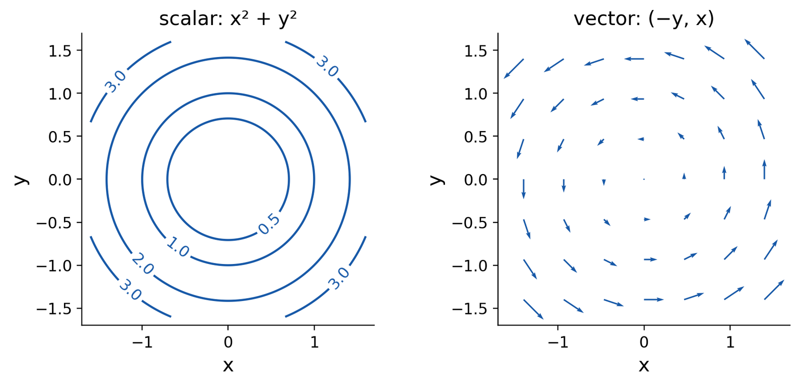
A scalar point function assigns one real number to each allowed position. Examples are temperature T(x,y,z), density ρ(x,y,z) and a model loss L(w₁,w₂).
A vector point function assigns a vector to each position:
F(x,y,z) = Pi+Qj+Rk.
The component functions P,Q,R may change independently. A field is defined on a stated domain; a singular formula does not define a value at its singular point.
Worked Example 3.1 – Evaluate a Field
For F=(xy,y²,z−x), at A=(1,2,3):
F(A) = (2,4,2).
Its magnitude is √(4+16+4)=2√6. The field value is a vector, while its magnitude is a scalar.
Worked Example 3.2 – A Radial Scalar
Let f=√(x²+y²+z²). Its domain is all space, and f gives distance from the origin. The function is continuous everywhere but is not differentiable at the origin.
A Field Is Not a Trajectory
An arrow plot shows possible local directions. A particle path requires a starting point and a motion law such as r′(t)=F(r(t)). The arrows alone do not give the time taken to travel.
Scalar Versus Vector Output
| Operation | Output |
|---|---|
| Magnitude of F | Scalar |
| Evaluate φ at a point | Scalar |
| Evaluate F at a point | Vector |
| Add two vector fields | Vector |
First Step
State the domain, identify the output type and write the field components before differentiating. These choices determine which later operations make sense.
2. Vector Algebra for Calculus
For a=(a₁,a₂,a₃) and b=(b₁,b₂,b₃), the dot product is a scalar:
a·b = a₁b₁+a₂b₂+a₃b₃.
It measures directional alignment. If θ is their angle and both vectors are nonzero:
a·b = |a||b|cos θ.
Perpendicular nonzero vectors have dot product zero.
The cross product is a vector perpendicular to both inputs. Its magnitude is the parallelogram area |a||b|sin θ, and its direction follows the right-hand rule.
Worked Example 3.3 – Dot and Cross Products
For a=(1,2,0), b=(0,1,3):
a·b = 2.
a×b = (6,−3,1).
The cross product dotted with either input is zero, which checks perpendicularity.
Unit Vectors and Projections
A nonzero vector a has unit direction a/|a|. A unit vector has magnitude one, not necessarily components equal to one.
Worked Example 3.4 – Normalise a Direction
For a=(2,−1,2), the magnitude is 3:
â = (2/3,−1/3,2/3).
The squared components sum to one. This normalisation is essential for a rate per unit distance.
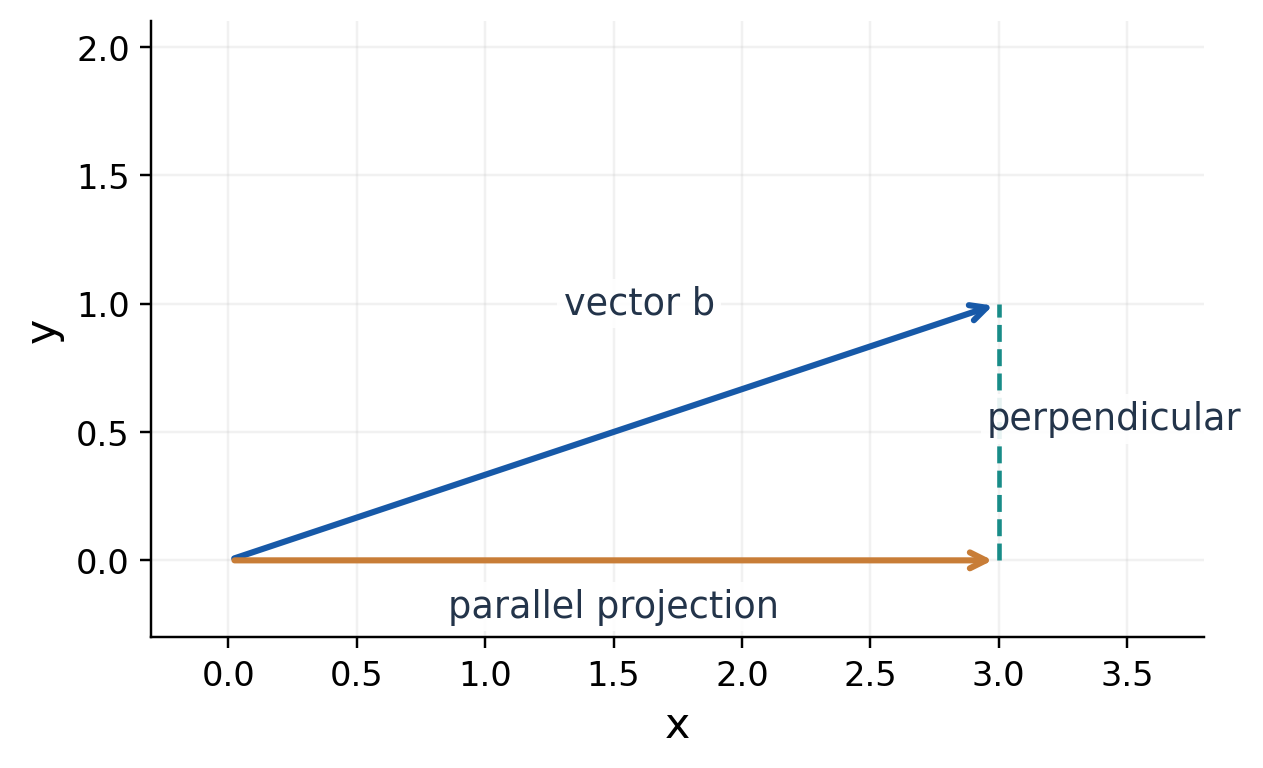
Worked Example 3.5 – Scalar Projection
For b=(3,1,0) and unit direction u=(1,1,0)/√2:
b·u = 4/√2 = 2√2.
The vector projection is (b·u)u=(2,2,0). The scalar projection and vector projection are different objects.

Cross-Product Order Matters
Reversing inputs changes sign:
b×a = −a×b.
The cyclic relations are i×j=k, j×k=i and k×i=j. Reversing any pair reverses the result.
Calculus Connection
Dot products produce directional derivatives, work and flux. Cross products produce normals, oriented area and curl-related geometry. Track the output type after every operation.
3. Differentiating Vector Functions
A vector function of one parameter is differentiated component by component:
r(t) = (x(t),y(t),z(t)).
r′(t) = (x′(t),y′(t),z′(t)).
For position, r′ is velocity and r″ is acceleration. Speed is |r′| and is therefore a scalar. It can stay constant while velocity changes direction.
Worked Example 3.6 – Polynomial Motion
Let r(t)=(t,t²,t³). Then:
v = (1,2t,3t²), a = (0,2,6t).
At t=1, velocity is (1,2,3), acceleration is (0,2,6), and speed is √14.


Product Rules for Vectors
For differentiable vector functions a(t),b(t) and scalar h(t):
d(ha)/dt = h′a+ha′.
d(a·b)/dt = a′·b+a·b′.
d(a×b)/dt = a′×b+a×b′.
In the cross-product rule, preserve the order of the factors. Cross products are not commutative.
Worked Example 3.7 – Constant Magnitude
If a(t)·a(t)=c² for a constant c, differentiate:
2a·a′ = 0.
Thus a is perpendicular to a′ wherever both are defined. A constant-length rotating vector changes in a perpendicular direction.
Worked Example 3.8 – Circular Motion
For r=(cos t,sin t,0), velocity is (−sin t,cos t,0) and acceleration is (−cos t,−sin t,0). Speed equals one, but velocity is not constant.
The dot product r·r′ is zero, confirming that the tangent to the unit circle is perpendicular to its radius.
Interpretation
Differentiate the vector first, then take its magnitude if speed is required. The derivative of |r| is generally not the same as |r′|.
4. Curves, Tangents and Arc Length
For a regular curve, r′(t)≠0. Its unit tangent is:
T(t) = r′(t)/|r′(t)|.
The arc-length element is ds=|r′(t)|dt when the parameter increases from a to b. The length is:
L = ∫[a,b] |r′(t)| dt.
The parameter t need not be physical time. The same geometric curve can be described with different parameter speeds.

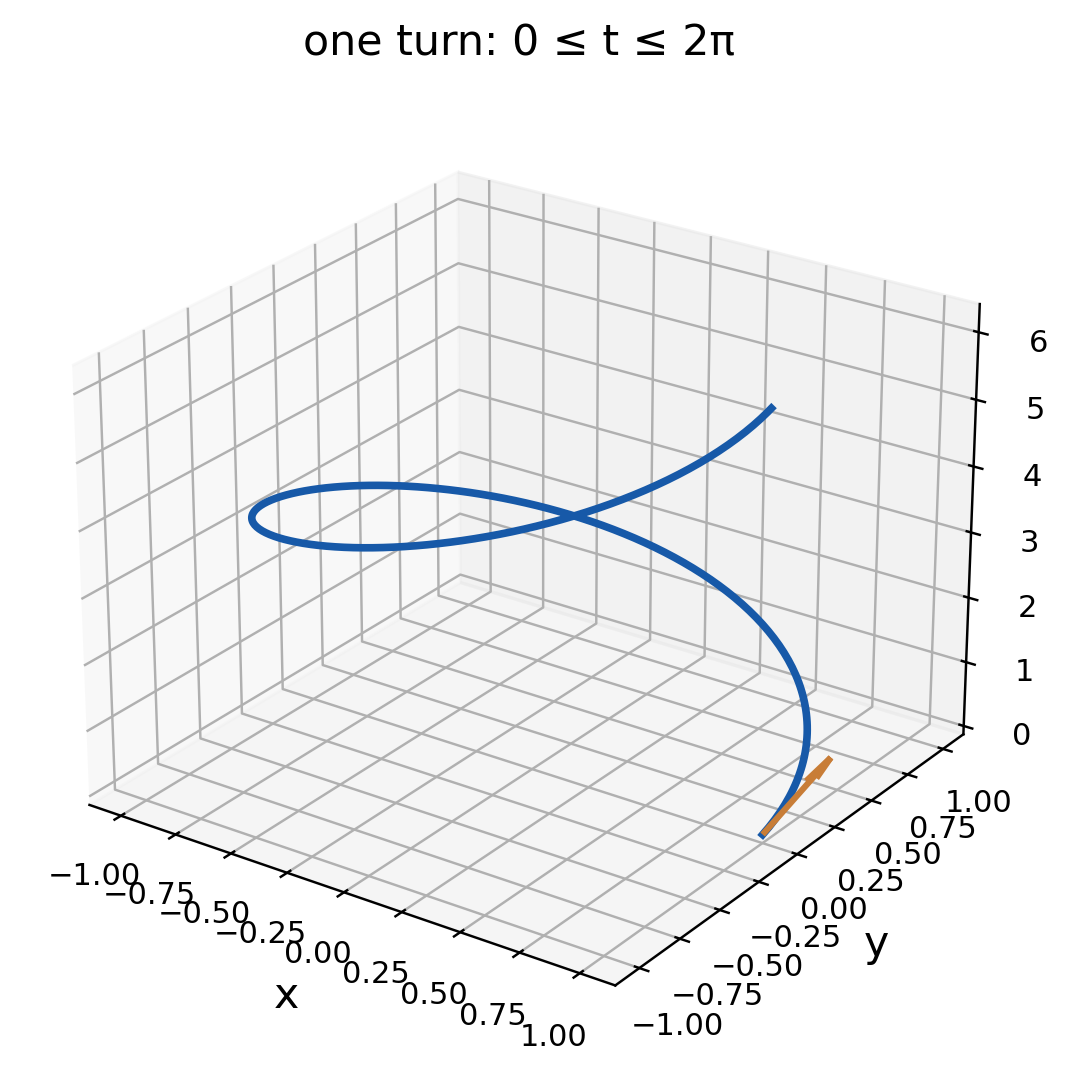
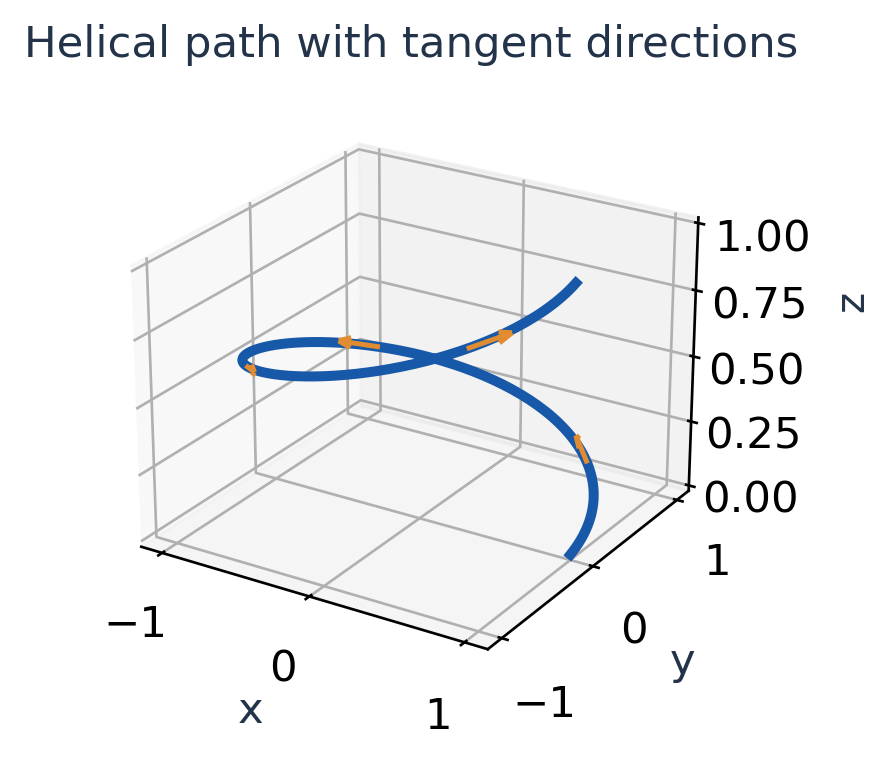
Worked Example 3.9 – A Helix
Velocity is (−sin t,cos t,1), with speed √2. Hence:
T = (−sin t,cos t,1)/√2.
Worked Example 3.10 – Tangent at the Start
For the helix at t=0, the point is (1,0,0) and velocity is (0,1,1). Thus:
T(0) = (0,1,1)/√2.
The tangent rises and moves in +y; it is not directed toward the helix’s final point. This separates a local tangent from a straight displacement joining distant points.
Length and Parameter Changes
For one turn, 0≤t≤2π:
L = ∫[0,2π] √2 dt = 2π√2.
Worked Example 3.11 – A Line Segment
From A=(0,0,0) to B=(2,1,2), use r(t)=t(2,1,2), 0≤t≤1. The derivative is constant (2,1,2), with magnitude 3.
L = ∫[0,1] 3 dt = 3.
This matches |B−A|. Reversing the path changes the tangent direction but does not change its length.
Worked Example 3.12 – Faster Parameterisation
The same segment is r(s)=s(1,1/2,1), 0≤s≤2. Its speed is 3/2 and its interval length is 2, again giving L=3.
Why Regularity Matters
At a point where r′=0, the formula for T divides by zero. The geometric curve may still have a tangent, but the parameterisation needs separate treatment or replacement near that point.
Before a Line Integral
Write r, its parameter interval, r′ and |r′|. Work uses r′ directly; scalar arc-length integrals use its magnitude.
5. The Del Operator
In Cartesian coordinates, del is the differential operator:
∇ = i∂/∂x+j∂/∂y+k∂/∂z.
It behaves like a vector of derivatives, but it is an operator, not a fixed ordinary vector. Its meaning depends on what follows it.
| Expression | Name | Input → Output |
|---|---|---|
| ∇φ | Gradient | Scalar → Vector |
| ∇·F | Divergence | Vector → Scalar |
| ∇×F | Curl | Vector → Vector |
The dot or cross symbol is part of the operation. Omitting it changes the meaning.
Worked Example 3.13 – Classify Expressions
For φ=x²+y²+z², ∇φ is a vector. For F=(x,y,z), ∇·F is the scalar 3, while ∇×F is the zero vector.
Calculate in Components
For F=(P,Q,R):
∇·F = Pₓ+Qᵧ+R_z.
∇×F = (Rᵧ−Q_z,P_z−Rₓ,Qₓ−Pᵧ).
For a scalar φ:
∇φ = (φₓ,φᵧ,φ_z).
Worked Example 3.14 – One Field, Two Derivatives
For F=(x²,y²,z²):
∇·F = 2x+2y+2z.
∇×F = (0,0,0).
Zero curl does not force zero divergence. The field expands locally except where the divergence happens to vanish.
Operator Scope
In ∇·(φF), the derivatives act on the product. It is generally incorrect to multiply φ by ∇·F and ignore the derivatives of φ. A product rule is needed.
Similarly, ∇(φψ) differentiates both scalar factors. Writing parentheses makes the intended scope clear.
Memory Guide
Gradient has no dot or cross and starts from a scalar. Divergence takes a dot and returns a scalar. Curl takes a cross and returns a vector.
A Zero Value Versus an Identity
For F=(x²,y²,z²), divergence is zero at (1,−1,0). It is not zero throughout an open neighbourhood, because moving slightly in x changes 2x+2y+2z.
Therefore the field is not solenoidal on all space, despite that single zero value. Curl, in contrast, vanishes identically for this field. Classification requires a domain-wide statement.
6. Gradient of a Scalar Field
For a differentiable scalar field φ:
∇φ = φₓi+φᵧj+φ_zk.
Each partial derivative holds the other coordinates fixed. The gradient gathers all first-order rates into one vector.
Worked Example 3.15 – A Polynomial Gradient
Let φ=x²y+yz². Then:
∇φ = (2xy,x²+z²,2yz).
At (1,2,1):
∇φ = (4,2,4), |∇φ| = 6.
The gradient’s unit direction is (2/3,1/3,2/3). Its magnitude is not the sum of the components; it is the square root of the sum of their squares.


Worked Example 3.16 – Exponential Field
For φ=e^(xy)+z²:
∇φ = (ye^(xy),xe^(xy),2z).
At (0,2,1), the gradient is (2,0,2). The y-component is zero at this point because x=0, even though φ depends on y elsewhere.
Worked Example 3.17 – Logarithmic Field
For φ=ln(x²+y²+z²), the domain excludes the origin:
∇φ = 2(x,y,z)/(x²+y²+z²).
The denominator comes from the logarithm’s derivative and must remain in all three components.
Linear Approximation
For a small displacement h=(h₁,h₂,h₃):
φ(A+h) ≈ φ(A)+∇φ(A)·h.
For the polynomial example at A=(1,2,1), a small displacement (0.01,0,−0.02) gives estimated change:
Δφ ≈ 4(0.01)+4(−0.02) = −0.04.
Gradient Check
After differentiating, count the components and check the domain. Substituting the point before taking partial derivatives would turn the function into a constant and lose the needed information.


7. Gradient and Level Geometry
A level surface φ(x,y,z)=c contains points with the same scalar value. If a differentiable curve stays on this surface, φ(r(t))=c.
The chain rule gives:
dφ(r(t))/dt = ∇φ·r′(t) = 0.
Thus the gradient is perpendicular to every tangent direction at a point where the level surface is regular and ∇φ≠0.

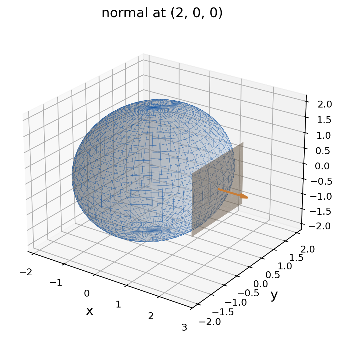
Worked Example 3.18 – A Sphere Normal
For φ=x²+y²+z², ∇φ=2(x,y,z). At A=(2,0,0), a normal is (4,0,0), so the tangent plane is x=2.
Gradient Points Uphill
For a unit direction u, the first-order change per unit distance is ∇φ·u. It is largest when u points along the gradient and smallest in the opposite direction.
Worked Example 3.19 – Two Level Directions
For f=x²+2y² at (1,1), the gradient is (2,4). A tangent direction to the level ellipse is (2,−1), because:
(2,4)·(2,−1) = 0.
The corresponding unit tangent is (2,−1)/√5. Motion along this direction has zero first-order change at the point; a straight line in that direction need not remain exactly on the ellipse.
A Critical-Point Caution
At the origin of f=x²+y², the gradient is zero. There is no unique steepest-increase unit direction determined by the gradient formula there, and the zero level set is a single point rather than a regular curve.
Orientation of Normals
Both ∇φ and −∇φ are normal. For a closed boundary, the outward choice depends on how the solid is described. The gradient of φ points toward increasing φ, which is outward for a sublevel solid φ≤c.
Geometry Check
The gradient is normal to a level set, not tangent to it. A nonzero gradient is the regularity condition needed for the usual tangent-plane construction.
8. Directional Derivatives
For a differentiable field φ and a unit vector u, the directional derivative at A is:
Dᵤφ(A) = ∇φ(A)·u.
It measures change per unit distance in the stated direction. A direction described by a nonzero vector a must first be converted to u=a/|a|.
Worked Example 3.20 – Normalise, Then Dot
For φ=x²y+yz² at (1,2,1), ∇φ=(4,2,4). Find the derivative in direction a=(2,−1,2).
Since |a|=3, u=(2,−1,2)/3:
Dᵤφ = (8−2+8)/3 = 14/3.
Using a directly would give 14, which is the change per unit parameter for displacement ta, not per unit distance.

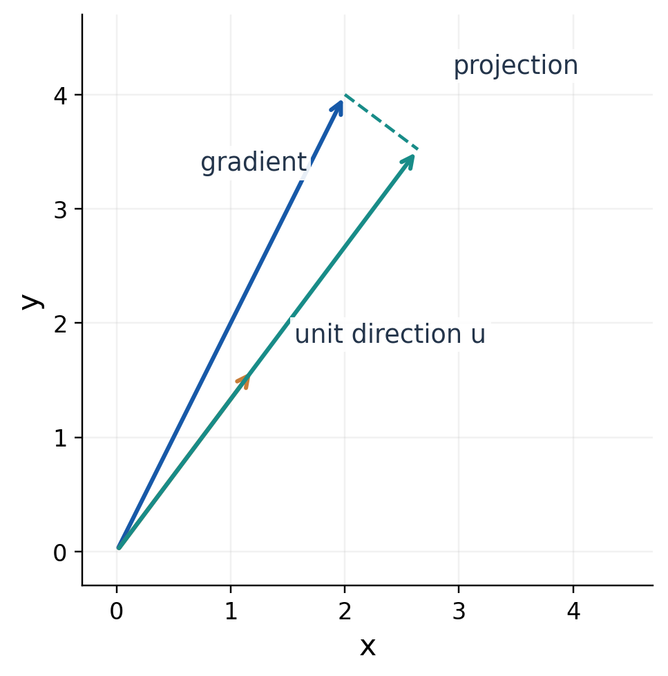
Worked Example 3.21 – From A Toward B
Let f=x²+2y², A=(1,1) and B=(4,5). The direction vector is B−A=(3,4), with magnitude 5.
∇f(A) = (2,4), u = (3/5,4/5).
Dᵤf = 6/5+16/5 = 22/5.
The derivative is evaluated at A. Do not average gradients at A and B; that would describe a different calculation.
Worked Example 3.22 – A Negative Derivative
At the same point, choose u=(−1,0). Then Dᵤf=−2. The function initially decreases in that direction.
Zero Derivative
A unit vector perpendicular to ∇f gives zero directional derivative. This means no first-order change in that direction at the point; second-order change may still occur.
Units
If φ is temperature and coordinates are distances, Dᵤφ has temperature-per-distance units. The gradient magnitude has the same units.
Answer Format
Write the gradient at the point, the normalised direction and their dot product. Keeping these three lines separate makes the method easy to verify.
9. Maximum and Minimum Rates
By the dot-product bound, for any unit direction u:
−|∇φ| ≤ Dᵤφ ≤ |∇φ|.
If ∇φ≠0, the maximum rate is |∇φ| in direction ∇φ/|∇φ|. The minimum rate is −|∇φ| in the opposite direction.
Worked Example 3.23 – Steepest Increase
For φ=x²y+yz² at (1,2,1), the gradient is (4,2,4) and its magnitude is 6.
The maximum directional derivative is 6 in unit direction (2/3,1/3,2/3). The minimum is −6 in the negative of that direction.

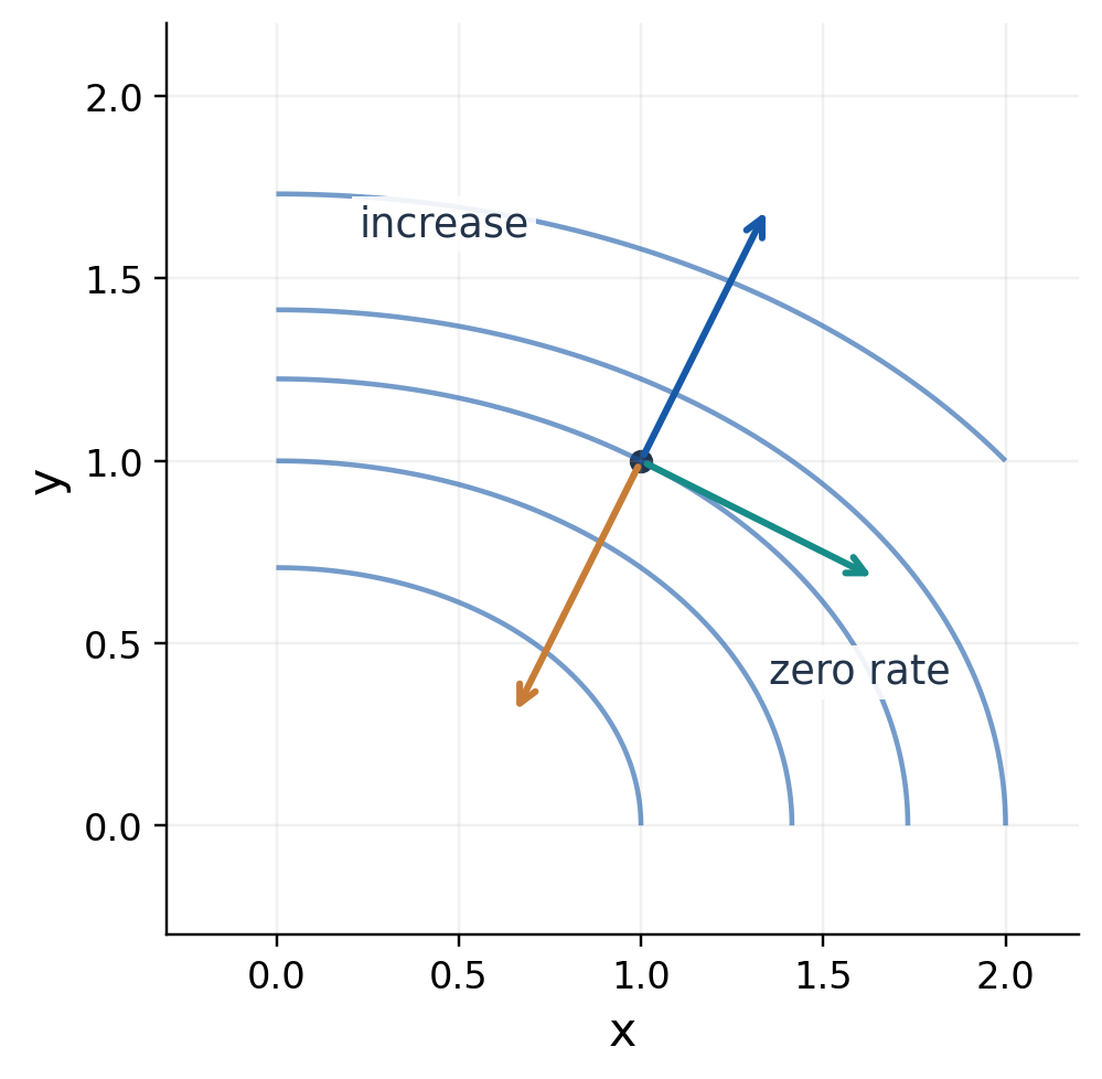
Worked Example 3.24 – Zero Rate in a Plane
For f=x²+2y² at (1,1), ∇f=(2,4). The unit directions perpendicular to it are:
u = ±(2,−1)/√5.
These are the two tangent directions to the level ellipse at that point.
Worked Example 3.25 – A Possible Rate
Can a unit direction produce rate 5? Here |∇f|=√20≈4.472. Since 5 exceeds the maximum possible rate, no such unit direction exists.
Worked Example 3.26 – Angle to the Gradient
For a desired rate √5, use Dᵤf=|∇f|cos θ. Hence:
cos θ = √5/(2√5) = 1/2.
The angle is π/3. In the plane there are two unit directions making that angle with the gradient.
At a Zero Gradient
All first directional derivatives are zero when the function is differentiable and its gradient is zero. This alone does not classify the point as a maximum or minimum; a saddle can also have zero gradient.
Rate Check
Before solving for a direction, compare the requested rate with the gradient magnitude. An impossible target can be rejected immediately.
10. Tangent Planes and Normal Lines
For a regular level surface φ(x,y,z)=c at A=(a,b,c₀), a normal vector is ∇φ(A). The tangent plane is:
∇φ(A)·(x−a,y−b,z−c₀) = 0.
A normal line is r=A+t∇φ(A). Any nonzero scalar multiple of the gradient gives the same plane and line.
Worked Example 3.27 – Ellipsoid Tangent Plane
Let x²+2y²+3z²=6 at A=(1,1,1). The point lies on the surface because 1+2+3=6.
∇φ(A) = (2,4,6).
2(x−1)+4(y−1)+6(z−1) = 0.
x+2y+3z = 6.

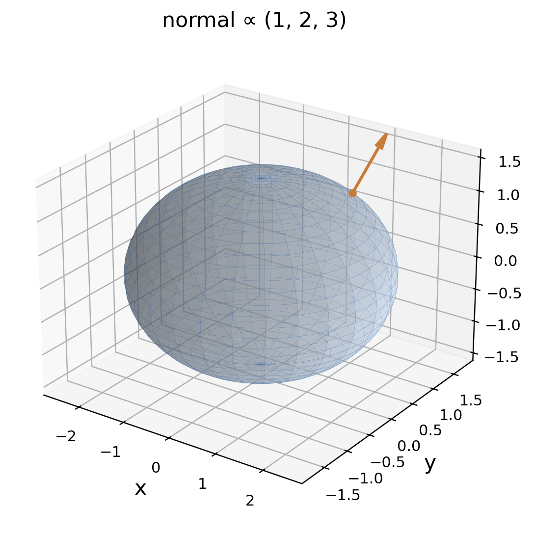
Normal Lines and Angles
For the ellipsoid, a normal line is:
(x,y,z) = (1,1,1)+t(1,2,3).
Worked Example 3.28 – Angle Between Surfaces
The surfaces φ=x²+y²+z² and ψ=x+y+z have normals ∇φ and ∇ψ. At A=(1,0,0), use normals n₁=(2,0,0), n₂=(1,1,1).
For the acute angle between their tangent planes:
cos θ = |n₁·n₂|/(|n₁||n₂|) = 1/√3.
The absolute value selects the acute angle. If oriented normals are requested instead, preserve the sign and the chosen directions.
A Graph as a Level Surface
For z=g(x,y), write φ=g(x,y)−z. Its gradient is (gₓ,gᵧ,−1); the opposite vector (−gₓ,−gᵧ,1) is upward-pointing.
This graph normal will reappear in surface-flux calculations. It is not yet a unit normal unless divided by its magnitude.
Plane Check
Verify that the point lies on the surface and then substitute it into the final plane equation. Both checks should succeed before the answer is accepted.
11. Gradient Product and Chain Rules
For differentiable scalar fields φ and ψ:
∇(φ+ψ) = ∇φ+∇ψ.
∇(φψ) = φ∇ψ+ψ∇φ.
For a differentiable one-variable function h:
∇[h(φ)] = h′(φ)∇φ.
These identities apply the ordinary product and chain rules to each partial derivative. Parentheses show which expression the operator acts on.
Worked Example 3.29 – Exponential of a Quadratic
Let φ=x²+y²+z². Then:
∇(e^φ) = 2e^(x²+y²+z²)(x,y,z).
The exponential factor multiplies every component.
Worked Example 3.30 – A Quotient Gradient
Let φ=x/y, defined where y≠0. Then:
∇φ = (1/y,−x/y²,0).
At (2,1,0), the gradient is (1,−2,0). The function does not depend on z, so its z-component is zero. The excluded plane y=0 remains outside the domain after differentiation.
Radial Gradient Formulas
Let r=√(x²+y²+z²), with r>0. Then:
∇r = (x,y,z)/r.
∇(rⁿ) = nr^(n−2)(x,y,z).
For a differentiable radial profile h(r):
∇h(r) = h′(r)(x,y,z)/r.
Worked Example 3.31 – Reciprocal Radius
For r>0:
∇(1/r) = −(x,y,z)/r³.
Worked Example 3.32 – Logarithmic Radius
∇(ln r) = (x,y,z)/r².
This differs by a factor of two from ∇ln(r²), because ln(r²)=2ln r for r>0.
Domain Caution
These radial derivative formulas use division by r. At the origin, a specific function may still be differentiable, but that requires a separate check. For example, r² has gradient 2(x,y,z) everywhere even though the derivation using ∇r excluded r=0.
Simplify After Checking
A derived formula may extend continuously to a previously excluded point, but the original function and its differentiability there must be examined explicitly.
12. Divergence of a Vector Field

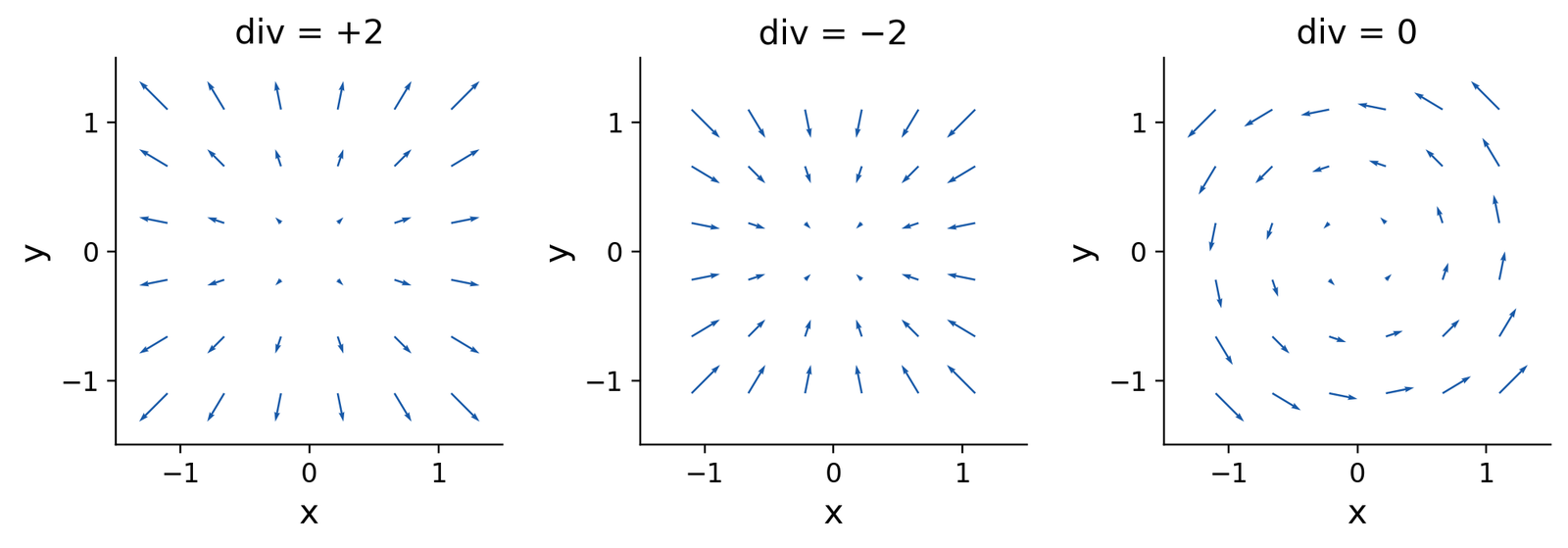
For F=(P,Q,R), divergence is the scalar:
∇·F = Pₓ+Qᵧ+R_z.
Differentiate each component with respect to its matching coordinate. Do not add all nine first partial derivatives.
Worked Example 3.33 – Polynomial Divergence
For F=(x²y,y²z,z²x):
∇·F = 2xy+2yz+2zx.
At (1,2,3), the value is 4+12+6=22.
Worked Example 3.34 – A Diagonal Linear Field
For F=(ax,by,cz), where a,b,c are constants:
∇·F = a+b+c.
The divergence is constant even though the field values vary with position.
Local Expansion and Compression
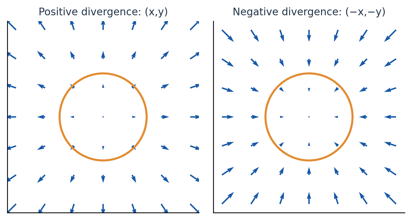
In a velocity field, positive divergence indicates local net expansion of an infinitesimal volume, while negative divergence indicates local net compression. Zero divergence means no local net volume creation under the stated smooth model.
Worked Example 3.35 – Source-Like Field
For F=(x,y,z), divergence is 3. The field points outward from the origin, and its outward flux through a small closed surface is positive.
Worked Example 3.36 – A Sink-Like Field
For F=(−x,−y,−z), divergence is −3. Reversing the field reverses its flux and its local expansion sign.
What Zero Does Not Mean
For F=(−y,x,0), divergence is zero, but the arrows circulate and the field is nonzero away from the z-axis. A divergence-free field need not be stationary or irrotational.
Units
If velocity has length/time units, a spatial derivative has units 1/time. Divergence is therefore a local relative volume-change rate, not a velocity vector.
Calculation Trick
Write Pₓ, Qᵧ and R_z on separate lines before adding. This prevents accidentally using Qₓ or Rᵧ merely because those derivatives are easier.

13. Divergence and Local Flux
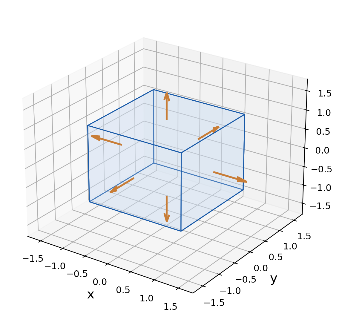
Divergence can be interpreted as outward flux per unit volume in the limit of a shrinking region around a point. This is a local interpretation; the full boundary-to-volume relation is Gauss’ theorem.
Worked Example 3.37 – A Small Cube
For F=(x,y,z), consider a cube centred at the origin with side 2h. On x=h, F·n=h and the face area is 4h², so its flux is 4h³.
On x=−h, the outward normal is −i, and F·n=(−h)(−1)=h. This face also contributes 4h³.
All six faces contribute equally, giving total flux 24h³. The cube volume is 8h³:
outward flux / volume = 3.
This equals ∇·F everywhere.
Worked Example 3.38 – A Numerical Cube Check
Choose h=1/2 in the small-cube example. The side length is 1, the volume is 1 and each face contributes 1/2.
Φ = 6(1/2) = 3.
Thus flux divided by volume is again 3. Shrinking the cube changes both quantities by the same cubic scale for this linear field.
Product Rule for Divergence
For a scalar φ and vector F:
∇·(φF) = ∇φ·F+φ∇·F.
Worked Example 3.39 – A Scalar-Weighted Radial Field
Let φ=x²+y²+z²=r² and F=(x,y,z). Then ∇φ=2(x,y,z) and div F=3.
∇·(r²F) = 2r²+3r² = 5r².
Directly, the field is (xr²,yr²,zr²). Differentiating each matching component gives the same answer.

Density and Velocity
If ρ is density and v is velocity, the flux field is ρv. Its divergence contains both ∇ρ·v and ρ div v. Ignoring the density gradient can change a transport calculation even when the velocity is divergence-free.
Sign Check
A negative x-coordinate on a left face does not automatically mean negative outward flux. Dot the field with that face’s outward normal before deciding the sign.
14. Solenoidal Vector Fields
A continuously differentiable vector field is called solenoidal on a domain when its divergence is zero throughout that domain:
∇·F = 0.
The condition is an identity over the domain, not merely a zero value at one point. For a smooth field on and inside a closed surface, it implies zero net outward flux through that surface.
Worked Example 3.40 – Determine a Parameter
Let F=(ax,2y,−3z). Its divergence is a+2−3=a−1. Thus the field is solenoidal precisely when a=1.
Worked Example 3.41 – A Nontrivial Solenoidal Field
For F=(yz,zx,xy), Pₓ=Qᵧ=R_z=0. Hence div F=0 everywhere, although the components are not constant.

Radial Fields Need a Domain Check
For r>0 and F=h(r)(x,y,z):
∇·F = 3h(r)+rh′(r).
Worked Example 3.42 – Inverse-Square Radial Field
Use h=r^(−3). Then h′=−3r^(−4), so:
∇·((x,y,z)/r³) = 0, r>0.
The field is solenoidal on its punctured domain. It is not defined at the origin.
Why This Matters for a Sphere
Its flux through a radius-a sphere centred at the origin is 4π, not zero. Gauss’ theorem cannot be applied across the missing origin with a zero divergence integral over the whole ball.
The hypothesis requires a smooth field on an open region containing the solid. That hypothesis fails here. There is no contradiction between the local calculation away from the origin and the nonzero sphere flux.
Linear-Field Shortcut
For F=A r with a constant matrix A, divergence equals the sum of the diagonal coefficients, or trace(A). Off-diagonal terms do not contribute to the matching-coordinate derivatives.
Solenoidal Check
Calculate the divergence, simplify it identically, then state the domain on which the result holds.
15. Curl in Cartesian Components
For F=(P,Q,R), curl is the vector:
∇×F = (Rᵧ−Q_z,P_z−Rₓ,Qₓ−Pᵧ).
The i-component compares derivatives in y and z; the j-component is P_z−Rₓ; the k-component is Qₓ−Pᵧ.
Worked Example 3.43 – A Polynomial Curl
Let F=(yz,xz,xy). Then:
Rᵧ−Q_z = x−x = 0.
P_z−Rₓ = y−y = 0.
Qₓ−Pᵧ = z−z = 0.
Thus curl F=0. In fact, this field is ∇(xyz).

Worked Example 3.44 – Mixed Polynomial Components
For F=(xy,yz,zx):
∇×F = (−y,−z,−x).
At (1,2,3), curl F=(−2,−3,−1). Meanwhile div F=x+y+z, so at the same point its divergence is 6.
The scalar divergence and vector curl describe different local features of the same field.
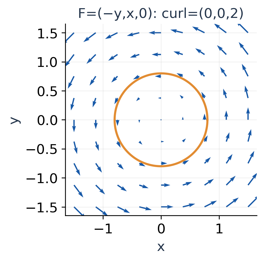
Worked Example 3.45 – A Rotational Linear Field
For F=(−y,x,0):
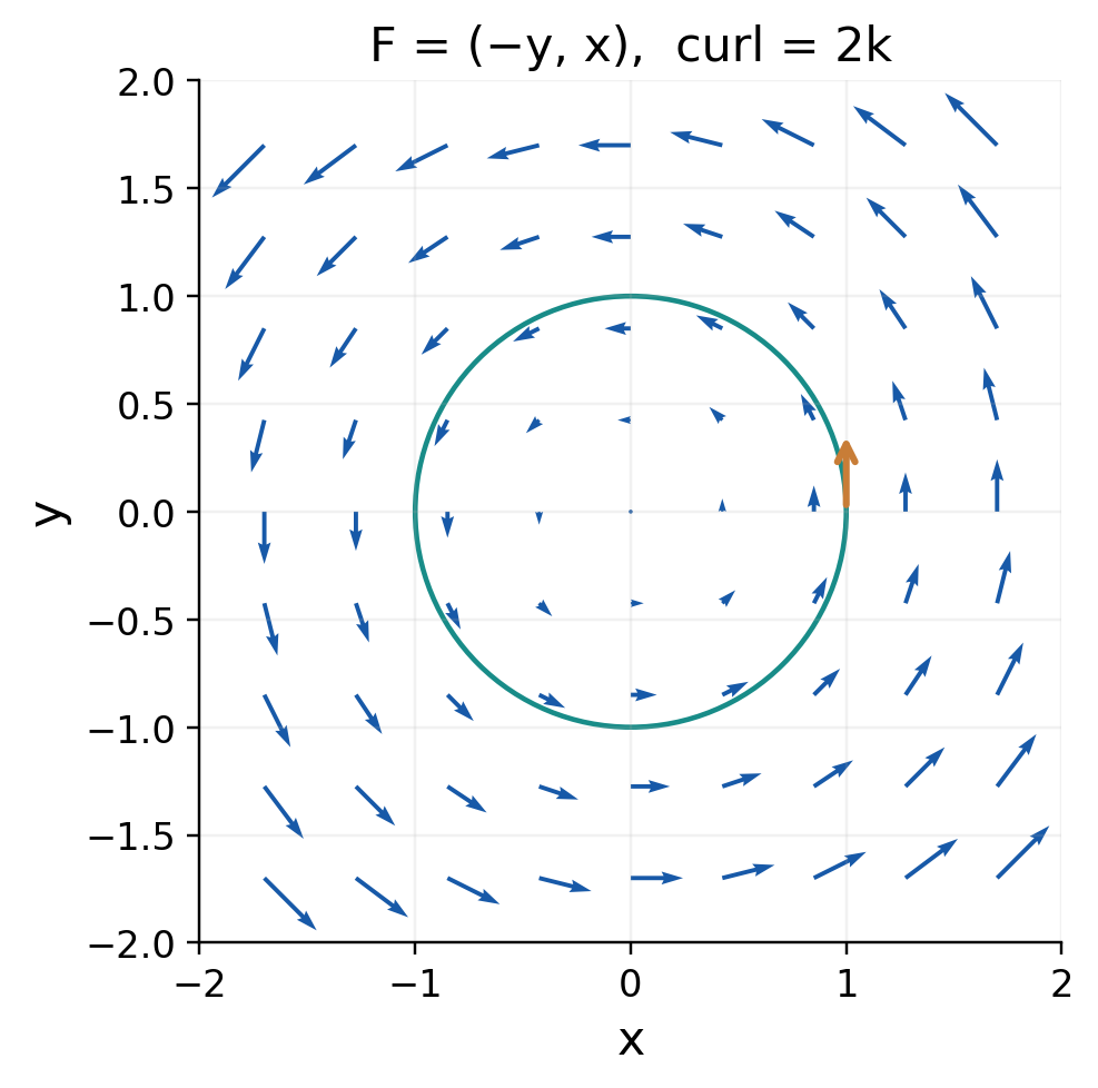
∇×F = (0,0,1−(−1)) = (0,0,2).
Its divergence is zero. This field rotates without local net expansion.
A Sign Memory Aid
The j-component is P_z−Rₓ. If using a determinant mnemonic, the middle cofactor carries a minus sign. Expanding that sign correctly gives exactly this component.
Zero Vector Versus Zero Scalar
Write curl F=(0,0,0) when showing component work. Writing simply 0 is conventional once the vector nature is clear, but it must not be confused with the scalar output of divergence.
Curl Check
For a field that visibly rotates anticlockwise in the xy-plane, a positive k-component is expected under the standard right-handed convention.

16. Curl and Local Rotation
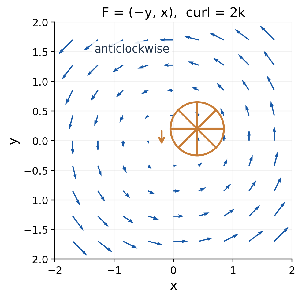
Curl measures local circulation density with an axis direction. In a velocity field corresponding to rigid rotation, the angular velocity is one-half the curl.
Worked Example 3.46 – Rotation at Angular Speed ω
Let F=(−ωy,ωx,0), with constant ω. Then:
∇×F = (0,0,2ω).
For ω>0, rotation is anticlockwise viewed from +z. For ω<0, both the rotation direction and curl direction reverse.

Circulation and Tangency
On a radius-a circle, F is tangent and has magnitude |ω|a. The positive circulation is 2πωa². Dividing by the disk area πa² gives 2ω, matching the normal curl component.
Worked Example 3.47 – Circulation of a Shear
For F=(y,0) around the unit square anticlockwise, the bottom segment contributes zero because y=0. The vertical sides have dx=0, so both contribute zero.
On the top, y=1 and x runs from 1 back to 0:
W = ∫[1,0] 1 dx = −1.
The negative circulation agrees with the negative k-curl component and the clockwise local wheel rotation.
Curl Is Local, Not a Path’s Shape
A curved trajectory alone does not prove nonzero curl. Streamlines can curve in an irrotational field. Conversely, a field can have nonzero curl even at a point where its value is zero.
Worked Example 3.48 – Rotation at the Origin
For F=(−y,x,0), the field value at the origin is zero, but curl F=(0,0,2) there. The local derivatives describe nearby rotation even though the central arrow has zero length.
Worked Example 3.49 – A Shear Field
Let F=(y,0,0). Then:
∇·F = 0, ∇×F = (0,0,−1).
The arrows are horizontal, with greater rightward speed at larger y. A small wheel rotates clockwise, consistent with the negative k-component.
Distinguish Three Ideas
- Field value: the local velocity or force vector.
- Divergence: local net expansion or compression.
- Curl: local circulation axis and magnitude.
A single arrow cannot reveal divergence or curl; both require information about nearby changes.
Interpretation Check
Do not infer curl merely from a large vector magnitude or from the visual bending of one path. Use derivatives or a local circulation argument.
17. Irrotational Fields
A continuously differentiable field is irrotational on a domain if its curl vanishes throughout that domain:
∇×F = 0.
Every sufficiently smooth gradient field is irrotational because mixed partial derivatives agree. The converse also needs a suitable domain condition for a global potential.
Worked Example 3.50 – A Parameter Condition
Let F=(ay,x,z). Its curl is (0,0,1−a), so it is irrotational precisely when a=1.
For a=1, one potential is φ=xy+z²/2, since ∇φ=(y,x,z).
Worked Example 3.51 – Another Gradient Field
F=(2x,2y,2z) has zero curl and potential φ=x²+y²+z². Its divergence is 6, so irrotational does not mean solenoidal.
Worked Example 3.52 – Both Conditions Together
For F=(yz,xz,xy), the field is ∇(xyz), so it is irrotational. Its divergence is also zero because each component is independent of its matching coordinate.
The field satisfies both conditions everywhere and is not constant. At (1,1,1) its value is (1,1,1). Neither “solenoidal” nor “irrotational” means that all field values vanish.
Curl-Free Plus an Appropriate Domain
A C¹ curl-free field on an open simply connected domain has a global scalar potential. Simply connected means that every closed loop can be continuously shrunk to a point within the domain.
The domain condition prevents a hidden hole from supporting nonzero circulation even when local curl is zero. A field’s formula and domain must be considered together.
Worked Example 3.53 – A Global Polynomial Field
F=(2xy,x²+2y,0) is defined on all space. Its curl is zero because Qₓ=Pᵧ=2x and the other cross partials vanish.
A potential is φ=x²y+y². This can be checked directly:
∇(x²y+y²) = (2xy,x²+2y,0).
Local Versus Global Statement
A curl-free field can have local potentials near ordinary points even when a single-valued global potential fails. The punctured-plane example in the domain-with-a-hole section illustrates the obstruction.
Classification
Test divergence and curl separately. A field may satisfy either condition, both conditions, or neither. Always state the domain for a claim about a potential.
A Quick Planar Compatibility Test
For F=(P,Q,0) independent of z, the only possible curl component is Qₓ−Pᵧ. A nonzero result disproves irrotationality immediately.
If this difference is zero, inspect the domain before claiming a global potential. On all of the plane, smooth polynomial examples have no missing-point obstruction; on a punctured domain, the same local test needs additional care.
18. Finding a Scalar Potential
To solve F=∇φ, compare φₓ=P, φᵧ=Q and φ_z=R. Integrate one component and retain an unknown function of the other variables.
Worked Example 3.54 – Recover the Potential
Let F=(2xy+z,x²+2y,x). First integrate P with respect to x:
φ = x²y+xz+g(y,z).
Differentiate this expression with respect to y and compare with Q:
φᵧ = x²+gᵧ = x²+2y.
Thus gᵧ=2y and g=y²+h(z). Now compare the z-derivative with R:
φ_z = x+h′(z) = x.
Therefore h is constant and:
φ = x²y+xz+y²+C.
Check Every Component
Differentiate the final potential. Its gradient is (2xy+z,x²+2y,x), exactly the original field. The arbitrary constant does not affect the gradient.
Worked Example 3.55 – Exponential Potential
For F=(eˣ cos y,−eˣ sin y,2z), integrate the first component:
φ = eˣ cos y+g(y,z).
Comparison with the second component gives gᵧ=0. Comparison with the third gives g_z=2z. Hence:
φ = eˣ cos y+z²+C.
Why the Unknown Function Matters
When integrating P with respect to x, a term depending on y or z differentiates to zero in x. It is therefore an arbitrary function g(y,z), not merely a numerical constant.
Dropping that function too early can make it impossible to recover the other field components correctly.
If Comparison Fails
If the required gᵧ unexpectedly depends on x, then either the field has no potential on the stated domain or an earlier differentiation or integration step is wrong. Check the curl to distinguish the possibilities.
Potential Method
Integrate one component, compare the others, determine the remaining functions, then differentiate the final answer back to all three components.
Potentials Differ by a Constant
On a connected domain, two differentiable potentials for the same field have zero gradient difference and therefore differ only by a constant.
For the polynomial example, adding 7 to φ changes neither its gradient nor any endpoint difference. The absolute numerical level of the potential is arbitrary; its changes determine the work under the F=∇φ convention.
19. A Domain with a Hole
Consider the planar field, extended independently of z:
F = (−y/(x²+y²),x/(x²+y²),0).
It is defined only where x²+y²>0. The z-axis is excluded. Its curl is zero at every point of its domain.
Worked Example 3.56 – Curl Away from the Axis
For the k-component:
Qₓ = (y²−x²)/(x²+y²)².
Pᵧ = (y²−x²)/(x²+y²)².
Their difference is zero; the other curl components also vanish.


Worked Example 3.57 – Unit-Circle Circulation
Use r(t)=(cos t,sin t,0), 0≤t≤2π. On this path:
F(r(t)) = (−sin t,cos t,0) = r′(t).
∮_C F·dr = ∫[0,2π] 1 dt = 2π.
A globally conservative field would give zero around every closed path. Therefore this field has no single-valued global potential on the full punctured domain.
Why Stokes’ Theorem Cannot Use the Disk
The unit disk intersects the excluded axis at its centre. The field is not smooth on an open region containing that disk, so the hypotheses fail. Inserting zero curl into a disk integral would be an invalid application.
A Local Angle Potential
On a suitable region avoiding a branch cut, an angle function can serve as a potential. However, the angle changes by 2π around one complete turn, so it cannot define one continuous single-valued potential on the entire punctured plane.
Domain Lesson
Zero curl is a local differential condition. A global potential also depends on the topology of the domain. Never skip the domain check when singularities are present.
20. Fundamental Differential Identities
For a twice continuously differentiable scalar field φ:
∇×(∇φ) = 0.
For a twice continuously differentiable vector field F:
∇·(∇×F) = 0.
The cancellation uses equality of mixed partial derivatives. The stated smoothness makes these identities valid in the ordinary classical sense used here.
Worked Example 3.58 – Curl of a Gradient
For φ=x²y+yz², ∇φ=(2xy,x²+z²,2yz). The curl components are 2z−2z, 0−0 and 2x−2x. All vanish.
Worked Example 3.59 – Divergence of a Curl
For F=(0,0,xy), curl F=(x,−y,0). Its divergence is 1−1=0.
Why Smoothness Is Stated
The mixed-derivative cancellations are justified when the second partial derivatives are continuous. For ordinary polynomials, exponentials and trigonometric combinations on their valid domains, this condition is straightforward to check.
At a singularity or a point defined by a special piecewise rule, do not assume the same cancellation without checking differentiability. An identity used outside its hypotheses cannot repair an undefined derivative.
Useful Product Identities
For smooth scalar φ and vector F:
∇×(φF) = ∇φ×F+φ(∇×F).
For smooth vector fields A and B:
∇·(A×B) = B·(∇×A)−A·(∇×B).
Worked Example 3.60 – Check a Curl Product
Take φ=x and F=(0,y,0). Then φF=(0,xy,0), whose curl is (0,0,y).
On the right, ∇φ=(1,0,0), so ∇φ×F=(0,0,y). The original field F has zero curl, so the second term is zero. Both sides agree.
Type Check
Curl of a gradient is a vector identity. Divergence of a curl is a scalar identity. Attempting ∇×(∇·F) is not the standard Cartesian curl operation because ∇·F is scalar.
Identity Habit
Record the output type and smoothness assumptions before using an identity. Product rules contain derivative terms from both factors; treating del as an ordinary constant vector loses them.
Worked Example 3.61 – Divergence of a Cross Product
Take A=(0,x,0) and B=(0,0,z). Then A×B=(xz,0,0), whose divergence is z.
The curls are curl A=(0,0,1) and curl B=0, so:
B·(∇×A)−A·(∇×B) = z.
Both sides agree. Reversing A and B would negate the cross product and the corresponding identity.
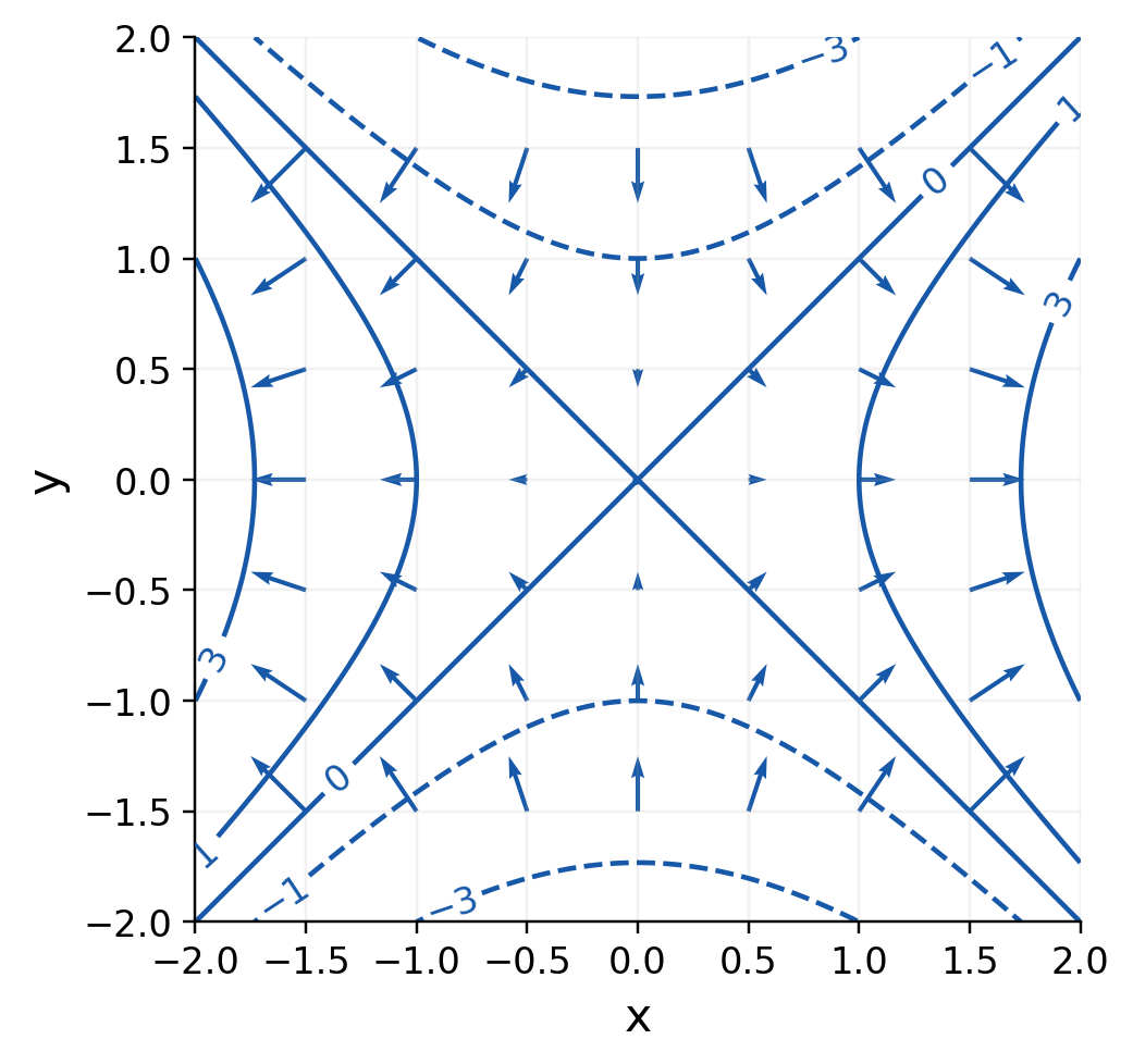
21. Laplacian of a Scalar Field
The Laplacian is divergence of the gradient:
∇²φ = ∇·∇φ = φₓₓ+φᵧᵧ+φ_zz.
Its output is scalar. A twice differentiable field satisfying ∇²φ=0 is called harmonic on its domain.
Worked Example 3.62 – A Harmonic Polynomial
For φ=x²+y²−2z²:
∇²φ = 2+2−4 = 0.
The gradient field (2x,2y,−4z) is therefore solenoidal and also irrotational.
Worked Example 3.63 – A Nonharmonic Polynomial
For φ=x²+y²+z², ∇²φ=6. The function is not harmonic on any open region.

Radial Laplacians
In three dimensions, for a smooth radial function h(r) with r>0:
∇²h(r) = h″(r)+(2/r)h′(r).
For h(r)=rⁿ:
∇²(rⁿ) = n(n+1)r^(n−2), r>0.
Worked Example 3.64 – Reciprocal Radius
Set n=−1. Then ∇²(1/r)=0 for r>0. The origin is excluded, so this is not a statement that 1/r is harmonic everywhere.
Worked Example 3.65 – Radius Itself
For n=1, ∇²r=2/r for r>0. The singular expression warns that the origin needs separate treatment.
Two Dimensions Differ
For a radial function of r=√(x²+y²) in the plane, the coefficient is 1/r rather than 2/r:
∇²h(r) = h″(r)+(1/r)h′(r).
Thus ln r is harmonic away from the planar origin, whereas its three-dimensional radial Laplacian is 1/r².
Dimension Check
A radial formula depends on the number of spatial dimensions. State whether r uses two coordinates or three before substituting.
22. Combined Operator Problems
Worked Example 3.66 – Classify a Field
Let F=(x²−y²,2xy,0). Its divergence is:
∇·F = 2x+2x = 4x.
Its curl has only a k-component:
Qₓ−Pᵧ = 2y−(−2y) = 4y.
Thus curl F=(0,0,4y). The field is neither solenoidal nor irrotational on all space, although the corresponding quantities vanish on particular planes.
A zero value at one point does not establish an identity on an open domain.
Worked Example 3.67 – A Gradient with Nonzero Divergence
For F=(2x,4y,6z), curl F=0 and div F=12. One potential is φ=x²+2y²+3z².
Worked Example 3.68 – A Cyclic Linear Field
Let F=(y,z,x). All matching-coordinate derivatives vanish, so div F=0. The curl is:
∇×F = (−1,−1,−1).
Thus the field is solenoidal but not irrotational. The curl magnitude is √3 everywhere, including the origin where the field itself is zero.
Classification Table
| Field | Divergence | Curl |
|---|---|---|
| (x,y,z) | 3 | (0,0,0) |
| (−y,x,0) | 0 | (0,0,2) |
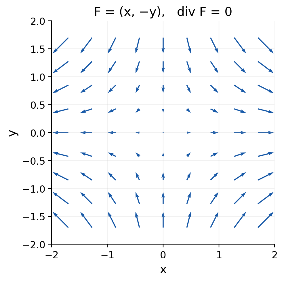
| (x,−y,0) | 0 | (0,0,0) |
| (xy,yz,zx) | x+y+z | (−y,−z,−x) |
The third example satisfies both conditions and is not constant. Its potential is (x²−y²)/2.
Worked Example 3.69 – A Scalar Multiplier
Let F=(x,−y,0) and φ=z. Since F is solenoidal:
∇·(zF) = ∇z·F = 0.
But the curl product gives:
∇×(zF) = k×(x,−y,0) = (y,x,0).
Multiplying by a nonconstant scalar can preserve one property and destroy another. Recheck the operator instead of assuming the original classification remains unchanged.
Exam Method
Find the divergence and all three curl components, simplify, and then classify. A table or separate labelled lines prevents mixing scalar and vector answers.
Worked Example 3.70 – Enforce Both Conditions
Let F=(ay,bx,cz), with constant a,b,c. Then:
∇·F = c, ∇×F = (0,0,b−a).
Both vanish precisely when c=0 and b=a. Under those conditions, φ=axy is a potential. The free parameter a can be nonzero, giving a family of nonconstant fields with both properties.
23. Integration of Vector Functions
A one-parameter vector function is integrated component by component:
∫F(t) dt = (∫P dt,∫Q dt,∫R dt)+C.
The integration constant is a constant vector. A definite integral produces a vector and needs no arbitrary constant.
Worked Example 3.71 – A Definite Vector Integral
Let F(t)=(2t,cos t,eᵗ), 0≤t≤1. Then:
∫[0,1] F(t) dt = (1,sin 1,e−1).
The three components are accumulated separately over the same interval.
Worked Example 3.72 – Recover Position
Suppose velocity v=(2t,1,3t²) and r(0)=(1,−1,2). Integration gives:
r(t) = (t²+C₁,t+C₂,t³+C₃).
The initial position fixes C=(1,−1,2).
Worked Example 3.73 – Net Displacement on an Arc
For v(t)=(cos t,sin t,0), 0≤t≤π:
∫[0,π] v(t) dt = (0,2,0).
The speed is one, so the distance travelled is π. The displacement magnitude is only 2. This is consistent with travelling along a semicircle rather than along its diameter.
Worked Example 3.74 – Initial-Value Motion
Let a=(0,2,0), v(0)=(1,0,0), r(0)=(0,0,0). First integrate acceleration:
v(t) = (1,2t,0).
Then integrate velocity:
r(t) = (t,t²,0).
At t=2, the particle is at (2,4,0). Its displacement is (2,4,0), but the distance travelled is the arc-length integral of √(1+4t²), which is a different quantity.
Integral Linearity
For constant scalars a,b:
∫(aF+bG) dt = a∫F dt+b∫G dt.
For a fixed vector c, one may also move it through a dot product or cross product while preserving order. A t-dependent vector cannot be treated as a constant without a product-rule argument.
Vector Integral Versus Work
Integrating F(t)dt componentwise returns a vector. Integrating F(r(t))·r′(t)dt returns scalar work. They are not interchangeable operations.
Initial Conditions
Each integration introduces its own vector constant. Apply velocity conditions after integrating acceleration, then apply position conditions after integrating velocity.
Average Velocity and Average Speed
In the preceding semicircle example, average velocity is (0,2/π,0), while average speed is 1.
The magnitude of average velocity is 2/π<1 because directions change during the motion. Integrating a vector and then taking its magnitude is generally different from integrating the magnitude. This distinction applies to transport and motion models alike.
24. Line Integrals and Parameterisation
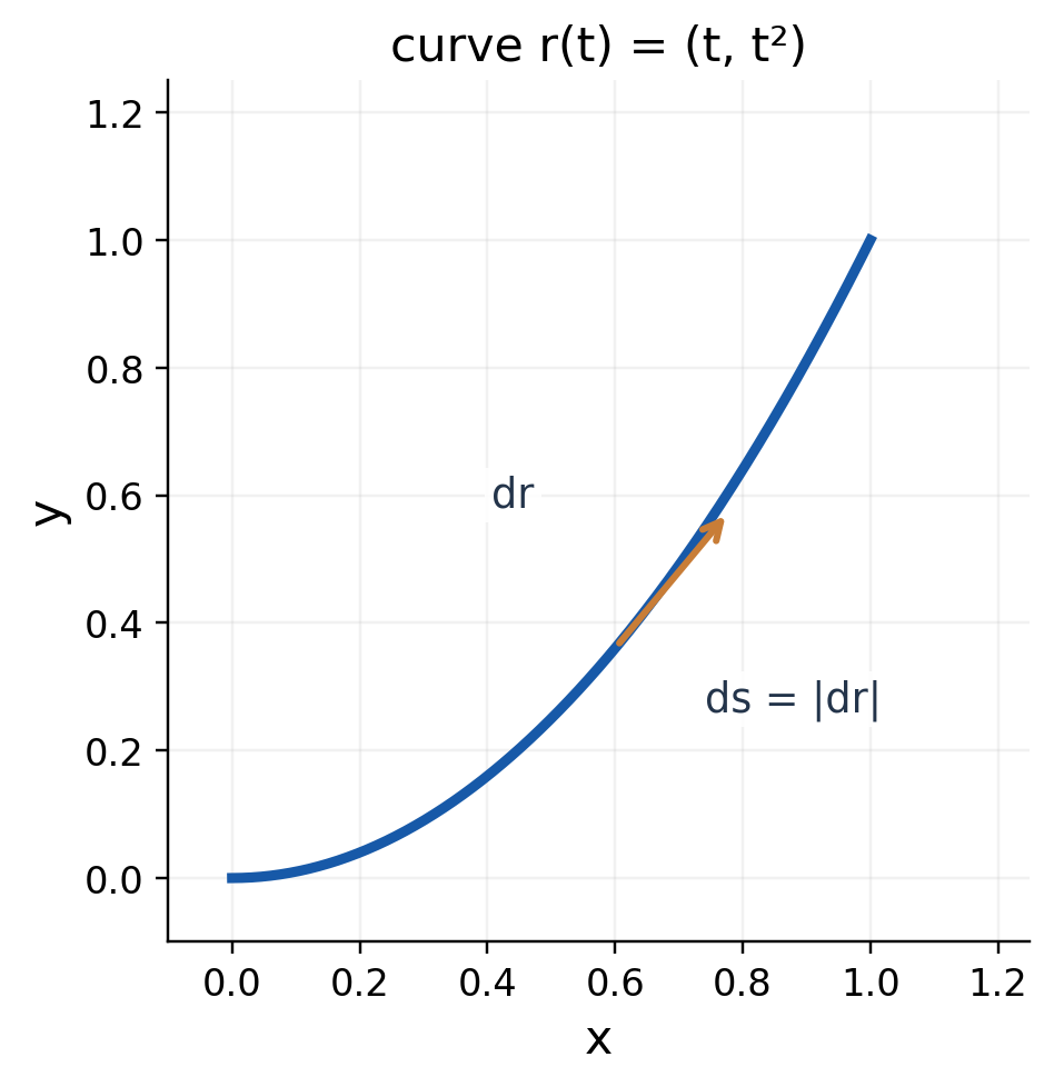
A curve C is described by r(t), a≤t≤b. Three related elements are:
dr = r′(t)dt, ds = |r′(t)|dt.
T ds = dr.
The first is oriented vector displacement. The second is nonnegative length. Their distinction controls the behaviour when the curve direction is reversed.
Common Parameterisations
| Curve | r(t) and Interval |
|---|---|
| Segment A to B | A+t(B−A), 0≤t≤1 |
| Radius-a circle, anticlockwise viewed from +z | (a cos t,a sin t,0), 0≤t≤2π |
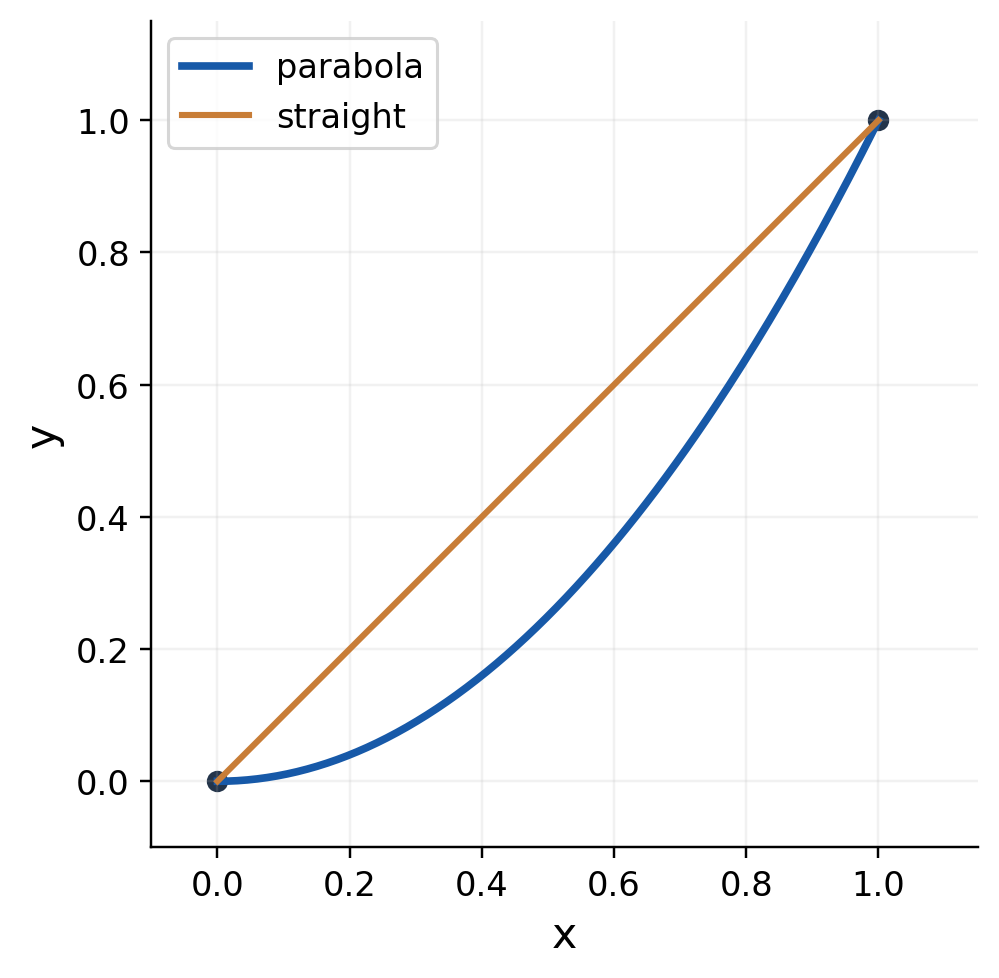
| Parabola from (0,0) to (1,1) | (t,t²,0), 0≤t≤1 |
| Helix, one turn | (cos t,sin t,t), 0≤t≤2π |
Two Kinds of Line Integral
A scalar line integral weights length:
∫_C f ds = ∫[a,b] f(r(t))|r′(t)| dt.
A vector-field work integral weights oriented displacement:
∫_C F·dr = ∫[a,b] F(r(t))·r′(t) dt.
Worked Example 3.75 – Constant Scalar on a Segment
For f=2 along the segment from (0,0,0) to (2,1,2), the length is 3. Thus ∫_C 2 ds=6 in either direction.
Worked Example 3.76 – Constant Vector on a Segment
For F=(1,2,0) along the same oriented segment:
W = F·(B−A) = 2+2 = 4.
Reversing the segment gives −4. The scalar length integral remains 6.

Parameter Checklist
Write the curve, interval, derivative and speed before substituting. This keeps work and arc-length calculations separate from the beginning.

25. Scalar Line Integrals
For f≥0, a scalar line integral can represent the mass of a wire with linear density f. More generally it accumulates a scalar quantity per unit length along a curve.
Worked Example 3.77 – A Circular Wire
Let C be the unit circle in the xy-plane and let f=x²+y². On C, f=1 and ds=dt under r=(cos t,sin t,0).
∫_C (x²+y²) ds = ∫[0,2π] 1 dt = 2π.
Worked Example 3.78 – Density Along a Segment
Let C run from (0,0) to (1,1) and f=x+y. Use r(t)=(t,t), 0≤t≤1, with speed √2.
I = ∫[0,1] (2t)√2 dt = √2.
The average density is 1 and the wire length is √2, giving the same mass.
Worked Example 3.79 – A Constant-Density Circle
A circular wire of radius 2 has length 4π. If its uniform linear mass density is 3, its mass is:
M = ∫_C 3 ds = 3(4π) = 12π.
The direction of traversal cannot change this mass. A negative answer would indicate an incorrect use of an oriented displacement instead of nonnegative arc length.
Worked Example 3.80 – Integrate x Along a Parabola
For r(t)=(t,t²), 0≤t≤1:
I = ∫[0,1] t√(1+4t²) dt.
Set u=1+4t², so du=8t dt:
I = (1/8)∫[1,5] u^(1/2) du = (5√5−1)/12.
The speed factor is essential. Using dt alone would give 1/2, which is not the arc-length-weighted integral.
Parameterisation Independence
A regular reparameterisation of the same curve does not change a scalar ds-integral. A faster parameter speed is compensated by the transformed speed factor and differential.
Reversing the Curve
The same scalar field integrated with ds gives the same value in the reverse direction. This remains true even when the scalar field takes negative values; orientation does not change ds.
Units
If f is mass per unit length, f ds has units of mass. An areal density would instead belong in a surface integral, not a wire integral.
Method
Substitute the scalar field and multiply by speed. For work integrals, use the dot product with velocity instead of speed alone.
26. Work Done by a Vector Field
For F=(P,Q,R), the work integral along an oriented curve is:
W = ∫_C P dx+Q dy+R dz.
Under r(t), this becomes the dot product F(r(t))·r′(t). The answer is scalar. A negative value means the field’s contribution opposes the chosen direction overall.
Worked Example 3.81 – A Parabolic Path
Let F=(y,x,0) and C be r(t)=(t,t²,0), 0≤t≤1.
F(r(t)) = (t²,t,0), r′ = (1,2t,0).
W = ∫[0,1] (t²+2t²) dt = 1.
The field is ∇(xy), and the endpoint potential difference is 1−0=1, confirming the calculation.

Worked Example 3.82 – Rotation Along a Quarter-Circle
Let F=(−y,x,0) and r(t)=(cos t,sin t,0), 0≤t≤π/2. Then F(r)=r′, with speed one.
W = ∫[0,π/2] 1 dt = π/2.
The field is tangent and aligned with the path, so the work is positive.
Worked Example 3.83 – A Radial Segment
For the same rotational field, use r(t)=(t,0,0), 0≤t≤1. The field along the path is (0,t,0), perpendicular to r′=(1,0,0).
W = ∫[0,1] 0 dt = 0.
A nonzero field can do zero work along a path if it remains perpendicular to displacement.
Common Substitution Error
The x-component P multiplies dx=x′dt; Q multiplies y′dt; R multiplies z′dt. Do not multiply every component by the same scalar speed or add the components before the dot product.
Work Check
Check the path direction, substitute all coordinates into F, calculate r′, take the dot product, and integrate over the stated interval.
27. Path Dependence Made Explicit
A line integral can depend on the entire route, not just the endpoints. To demonstrate path dependence, calculate the same field between the same points along two different paths.
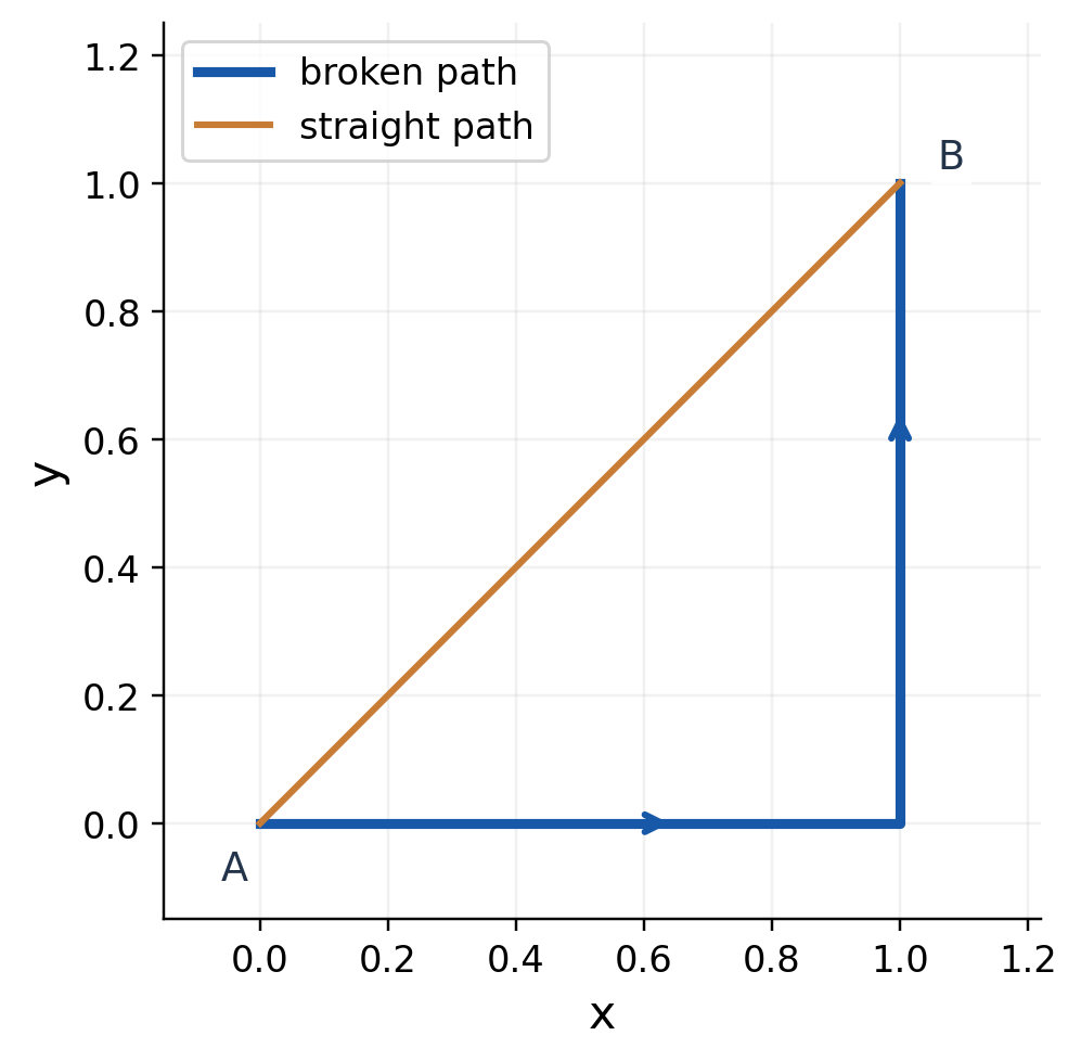
Worked Example 3.84 – Two Paths, Different Work
Take F=(−y,x,0), A=(0,0,0), B=(1,1,0).
For the straight path r(t)=(t,t,0), F=(−t,t,0), r′=(1,1,0), so the dot product is zero. Hence W₁=0.
For the broken path A→(1,0,0)→B, the first segment has zero work. On the second, x=1, y=t and dr=(0,1,0)dt:
W₂ = ∫[0,1] 1 dt = 1.
Since W₁≠W₂, the field is not conservative.
Worked Example 3.85 – A Third Route
For F=(−y,x), travel from A vertically to (0,1), then horizontally to B=(1,1). The first segment has zero work.
On the second, y=1 and x increases from 0 to 1:
W = ∫[0,1] (−1) dx = −1.
The three routes now give −1, 0 and +1 between the same endpoints. The route matters for this field.
Closed-Loop Interpretation
Follow the broken path from A to B, then return along the straight path. The resulting triangle is traversed anticlockwise viewed from +z.
The closed circulation is W₂−W₁=1. Its area is 1/2, and the normal curl component is 2, so curl times area also gives 1.

What the Example Proves
A single pair of unequal work values disproves path independence. A single pair of equal values does not prove it; a nonconservative field can give equal work along some specially chosen paths.
Endpoint Shortcut Requirements
Use a potential difference only after finding a potential or otherwise establishing conservativeness on the relevant domain. It is not valid merely because the endpoints are easy to evaluate.
Comparison Habit
Keep the endpoints and field identical when testing path dependence. Changing the field or endpoints would not provide the required comparison.
28. Conservative Work and Potentials
If F=∇φ on a domain and C runs from A to B within it, then:
∫_C F·dr = φ(B)−φ(A).
This is the fundamental theorem for line integrals. Work is independent of the path, and every closed-path integral is zero.
Worked Example 3.86 – A Spatial Potential
For F=(2xy+z,x²+2y,x), a potential is φ=x²y+xz+y².
Take A=(0,0,0), B=(1,2,3). Then:
W = φ(B)−φ(A) = 2+3+4 = 9.
No detailed parameterisation is needed, provided the path stays inside the field’s domain, which here is all space.
Worked Example 3.87 – Check the Spatial Straight Path
For the polynomial potential, use r(t)=(t,2t,3t), 0≤t≤1. Along it, φ=2t³+7t².
dφ(r(t))/dt = 6t²+14t.
W = ∫[0,1] (6t²+14t) dt = 9.
This directly confirms the endpoint result. The potential method avoided substituting and simplifying all three field components separately.
Worked Example 3.88 – An Exponential Potential
For φ=eˣ cos y+z², integrate ∇φ from A=(0,0,0) to B=(ln 2,0,1):
W = (2+1)−1 = 2.
Worked Example 3.89 – A Closed Curve
For F=∇(x²+y²+z²), any closed piecewise smooth curve has:
∮_C F·dr = 0.
The field need not vanish along the curve. The net work cancels because the potential returns to its initial value.
Potential Sign Convention
In mathematics, F=∇φ is a convenient definition of a scalar potential. In mechanics a potential energy U is often defined by F=−∇U. Then the work is U(A)−U(B).
State the convention instead of changing signs silently. Both descriptions agree if φ=−U.
Conditions Along a Path
The potential must be differentiable on a suitable region containing the path. A path crossing a point where F or φ is undefined is not rescued by an endpoint subtraction.
Short Solution Standard
Name the potential, verify its gradient when needed, evaluate both endpoints, and subtract final minus initial under the F=∇φ convention.
Reverse Endpoints Deliberately
The work from B back to A in the polynomial example is −9 for every admissible return path. Traversing any A-to-B path and any B-to-A path creates a closed curve with total work zero.
This cancellation concerns the signed work, not the total distance travelled or the absolute magnitude of force along the route.
29. Closed Curves and Orientation
A closed curve begins and ends at the same point. It is simple if it does not cross itself, apart from the repeated endpoint. A positive boundary orientation is always relative to a chosen normal.
For a planar curve viewed from +z, anticlockwise traversal corresponds to the upward normal k. Clockwise traversal corresponds to −k.
Worked Example 3.90 – A Circular Circulation
For F=(−y,x,0) around a radius-a circle anticlockwise:
r = (a cos t,a sin t,0), 0≤t≤2π.
F·r′ = a².
∮_C F·dr = 2πa².
The result reverses sign if the traversal is reversed.


Worked Example 3.91 – Reverse the Circle
Use r(t)=(a cos t,−a sin t,0), 0≤t≤2π. The path is clockwise viewed from +z and F·r′=−a², giving −2πa².
The curve length remains 2πa in either direction. Only the oriented displacement integral changes sign.
Multiple Boundary Components
For a horizontal annulus with upward normal, the outer circle is anticlockwise and the inner circle is clockwise. This makes the surface stay on the left as the boundary is traversed.
The inner boundary is not given the same direction as the outer boundary. Doing so would break the orientation pairing used by Stokes’ theorem.
Segment-by-Segment Integration
For a piecewise smooth boundary, calculate each oriented segment and add the results. The final endpoint of one segment should match the initial endpoint of the next.
A small arrow on every segment is often the clearest way to prevent an accidental reversal.
Right-Hand Rule
Point the right thumb along the chosen normal. The curled fingers indicate the positive boundary direction. State the viewing direction when using “clockwise” or “anticlockwise.”
30. Surface Integration Essentials
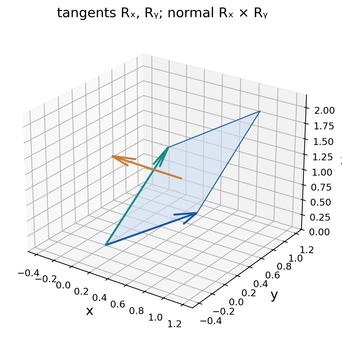
A surface can be parameterised by R(u,v). Its tangent vectors are Rᵤ and Rᵥ. Their cross product gives an oriented area factor:
dS_vector = (Rᵤ×Rᵥ) du dv.
dS = |Rᵤ×Rᵥ| du dv.
A scalar surface integral uses f dS. A vector flux integral uses F·dS_vector, with the selected orientation.
Worked Example 3.92 – A Planar Patch
Take R(u,v)=(u,v,1), 0≤u≤1, 0≤v≤2. Then Rᵤ×Rᵥ=(0,0,1). The surface area is 2.
For F=(0,0,3), its upward flux is 3×2=6. Reversing the normal gives −6.

Graph Surfaces Are Convenient
For z=g(x,y), parameterise R(x,y)=(x,y,g). Then:
Rₓ×Rᵧ = (−gₓ,−gᵧ,1).
dS = √(1+gₓ²+gᵧ²) dx dy.
The cross product is upward because its k-component is +1. For downward orientation, negate the vector.
Worked Example 3.93 – A Tilted Rectangle
For z=x+y over the unit square, the area factor is √3:
A_S = ∫[0,1] ∫[0,1] √3 dy dx = √3.
The projected xy-area is only 1. A sloping surface and its projection have different areas.
Unit Normal Versus Vector Area
The upward unit normal is (−gₓ,−gᵧ,1)/√(1+gₓ²+gᵧ²). Multiplying it by dS cancels the square-root denominator and gives the compact vector-area formula.
Do not use the nonunit normal and then multiply by the full dS again; that would count the area scale twice.
Surface Checklist
Choose the normal, parameterise the surface, calculate a cross product, and decide whether the problem needs its magnitude or its oriented vector form.

31. Flux Through a Graph
For F=(P,Q,R) and an upward graph z=g(x,y):
∬_S F·n dS = ∬_D (−Pgₓ−Qgᵧ+R) dx dy.
Evaluate P,Q,R on the surface z=g(x,y). For downward orientation, reverse the overall sign.
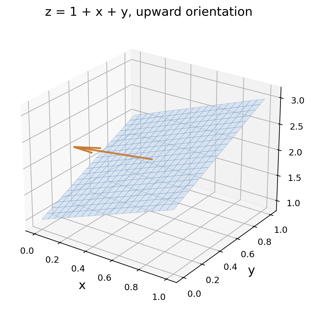
Worked Example 3.94 – Flux Through an Inclined Plane
Let F=(x,y,z), and S be z=1+x+y over the unit square with upward orientation. The vector area is (−1,−1,1)dx dy.
Substitute z=1+x+y into F:
F·(−1,−1,1) = −x−y+(1+x+y) = 1.
Thus the upward flux is 1.

Worked Example 3.95 – A Nonconstant Flux Density
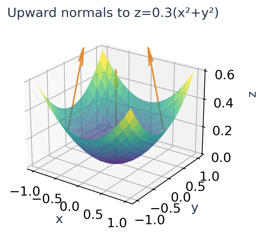
Let F=(0,0,z) through the upward graph z=x²+y² over the unit disk. Since only the k-component is nonzero, the dot product with (−2x,−2y,1) is z=r².
Φ = ∬_D (x²+y²) dA.
Φ = ∫[0,2π] ∫[0,1] r³ dr dθ = π/2.
The surface itself is curved, but its vector-area expression makes the calculation a simple double integral over its disk projection.
Scalar Area Integral Differs
The surface area would integrate √(1+4x²+4y²), not r². The flux value π/2 is therefore not the area of this paraboloid patch.
A Constant Field Can Have Zero Flux
A field tangent to a surface has F·n=0. For example, F=(1,0,0) through a horizontal plane has zero flux regardless of the plane’s area.
Sign Check
Before integration, inspect whether the field generally crosses with or against the chosen normal. The sign of the dot product gives the local contribution.
32. Flux Through a Sphere
For a sphere x²+y²+z²=a², a>0, the outward unit normal is:
n = (x,y,z)/a.
Its total area is 4πa². A radial field often has a constant normal component on the sphere, allowing a direct calculation.
Worked Example 3.96 – Radial Linear Field
For F=(x,y,z):
F·n = (x²+y²+z²)/a = a.
Φ = a(4πa²) = 4πa³.
The field strength grows with a, while the sphere area grows with a², explaining the cubic scaling.


Worked Example 3.97 – Constant Vector Field
For F=(0,0,1), the outward flux through a full sphere is zero. Upper and lower contributions cancel because F·n=z/a is odd in z.
A zero net flux does not mean the local flux is zero everywhere. The upper hemisphere has positive flux and the lower hemisphere has negative flux.
Worked Example 3.98 – Inverse-Square Radial Field
For F=(x,y,z)/r³, the normal component on r=a is 1/a². Hence:
Φ = (1/a²)(4πa²) = 4π.
This direct surface calculation is valid because the field is smooth near the sphere. Applying Gauss’ theorem to the whole enclosed ball would be invalid because the field is undefined at the origin.
Inward Orientation
Negating the outward normal negates every flux result: −4πa³ for the linear radial field and −4π for the inverse-square field.
Sphere Shortcut
Calculate F·n on the boundary first. Only if that scalar is constant may it be multiplied directly by the total surface area.
33. Closed Surfaces and Separate Pieces
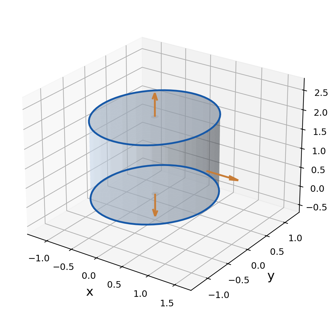
A closed surface surrounds a volume without an open edge. For a cylinder, the curved side alone is not closed; both caps must also be included.
For outward orientation, the top cap points upward, the bottom cap points downward, and the side normal points radially outward.

Worked Example 3.99 – Constant Vertical Field
For F=(0,0,1), a cylinder of radius a and height h has zero side flux. The top contributes πa²; the bottom contributes −πa².
The total outward flux is zero. Omitting the bottom would give a different, open-surface problem.
Worked Example 3.100 – Linear Radial Field
For F=(x,y,z), take radius a and 0≤z≤h. On the side, n=(cos θ,sin θ,0), so F·n=a.
The side area is 2πah, giving side flux 2πa²h. The top has z=h and normal k, so its flux is πa²h. The bottom has z=0, giving zero flux.
Φ_total = 2πa²h+πa²h = 3πa²h.
The divergence is 3 and the enclosed volume is πa²h, matching the total.
How to Close an Open Surface
Sometimes an open cap or side is easier to handle by adding a simple missing face. Calculate the flux through the closed surface using Gauss’ theorem, then subtract the added face with its outward orientation.
Edge Conventions
Edges shared by surface pieces do not contribute extra area to a flux integral. They matter for boundaries and orientations, but should not be counted as additional faces.
Closed-Surface Audit
List every boundary piece and its outward normal before applying a theorem. A missing cap is one of the most common flux errors.
34. Stokes’ Theorem
Let S be an oriented piecewise smooth surface with simple closed boundary C. Let F have continuous first partial derivatives on an open region containing S. With the positively paired boundary orientation:
∮_C F·dr = ∬_S (∇×F)·n dS.
The theorem equates circulation around the boundary with curl flux through the surface. It is used here without proof.

Worked Example 3.101 – A Unit Normal Curl
For F=(−y/2,x/2,0), curl F=k. Around a radius-a circle with upward paired orientation:
∮_C F·dr = ∬_D 1 dA = πa².
Halving the original rotational field halves its curl and its circulation. This checks linearity on both sides of Stokes’ theorem.
How to Apply Stokes’ Theorem
- Step 1: Identify the boundary curve and its traversal direction.
- Step 2: Choose a spanning surface with that same boundary.
- Step 3: Select a normal paired with the traversal.
- Step 4: Calculate curl F.
- Step 5: Integrate its normal component over the surface.
Worked Example 3.102 – A Constant Curl
For F=(−y,x,0) and C the radius-a circle anticlockwise viewed from +z, choose the upward disk.
∇×F = (0,0,2).
∮_C F·dr = 2∬_D 1 dA = 2πa².
This agrees with direct parameterisation.
Why a Different Surface May Help
A curved cap and a flat disk can share the same boundary. If the field is smooth on suitable neighbourhoods of both surfaces and the orientations match, both curl-flux integrals equal the same circulation.
The replacement surface must avoid any excluded singularities. Stokes’ theorem does not permit spanning a hole through a point where the field is undefined.
Pairing Rule
An upward disk uses an anticlockwise boundary viewed from above. Reverse both together if the curve is specified clockwise.


35. Stokes on a Planar Disk
Worked Example 3.103 – A Field with a z-Component
Let F=(−y,x,x²+y²). Let C be the unit circle in z=0, anticlockwise viewed from +z.
Its curl is:
∇×F = (2y,−2x,2).
Choose the upward unit disk, whose normal is k. Only the k-component contributes:
∮_C F·dr = ∬_D 2 dA = 2π.
The other curl components are not zero, but they are perpendicular to the selected normal and therefore contribute no flux through the disk.


Verify Directly Around the Boundary
Use r(t)=(cos t,sin t,0). On the unit circle, x²+y²=1:
F(r(t)) = (−sin t,cos t,1).
r′(t) = (−sin t,cos t,0).
Their dot product is sin²t+cos²t=1, so the circulation is the integral of 1 over 0≤t≤2π, giving 2π.
The z-component of F does not contribute because dz=0 on this horizontal boundary. This is consistent with the surface calculation rather than a reason to omit it when first computing curl.
Worked Example 3.104 – Radius Two
If the boundary radius becomes 2 while the field is unchanged, the disk area is 4π and the normal curl remains 2. The circulation becomes 8π.
Orientation Reversal
For the clockwise unit circle viewed from +z, use the downward disk normal. The answer is −2π. Keeping the upward normal with the clockwise boundary would give an inconsistent theorem setup.
Efficiency
When the boundary is horizontal, check whether the k-component of curl is simple. A flat spanning disk often avoids a long trigonometric line integral.
36. Stokes on a Slanted Triangle
Worked Example 3.105 – A Tilted Boundary
Let F=(z,x,y), and let C traverse A=(0,0,1), B=(1,0,0), C₀=(0,1,0), then A. The spanning triangle lies on x+y+z=1.
Its xy-projection is x,y≥0,x+y≤1. The projected traversal is anticlockwise, so choose the upward vector area (1,1,1)dx dy.
∇×F = (1,1,1).
(∇×F)·(1,1,1) = 3.
∮_C F·dr = 3(1/2) = 3/2.
The projected area is 1/2. The actual triangle area is √3/2, and its unit normal is (1,1,1)/√3; these factors give the same result.

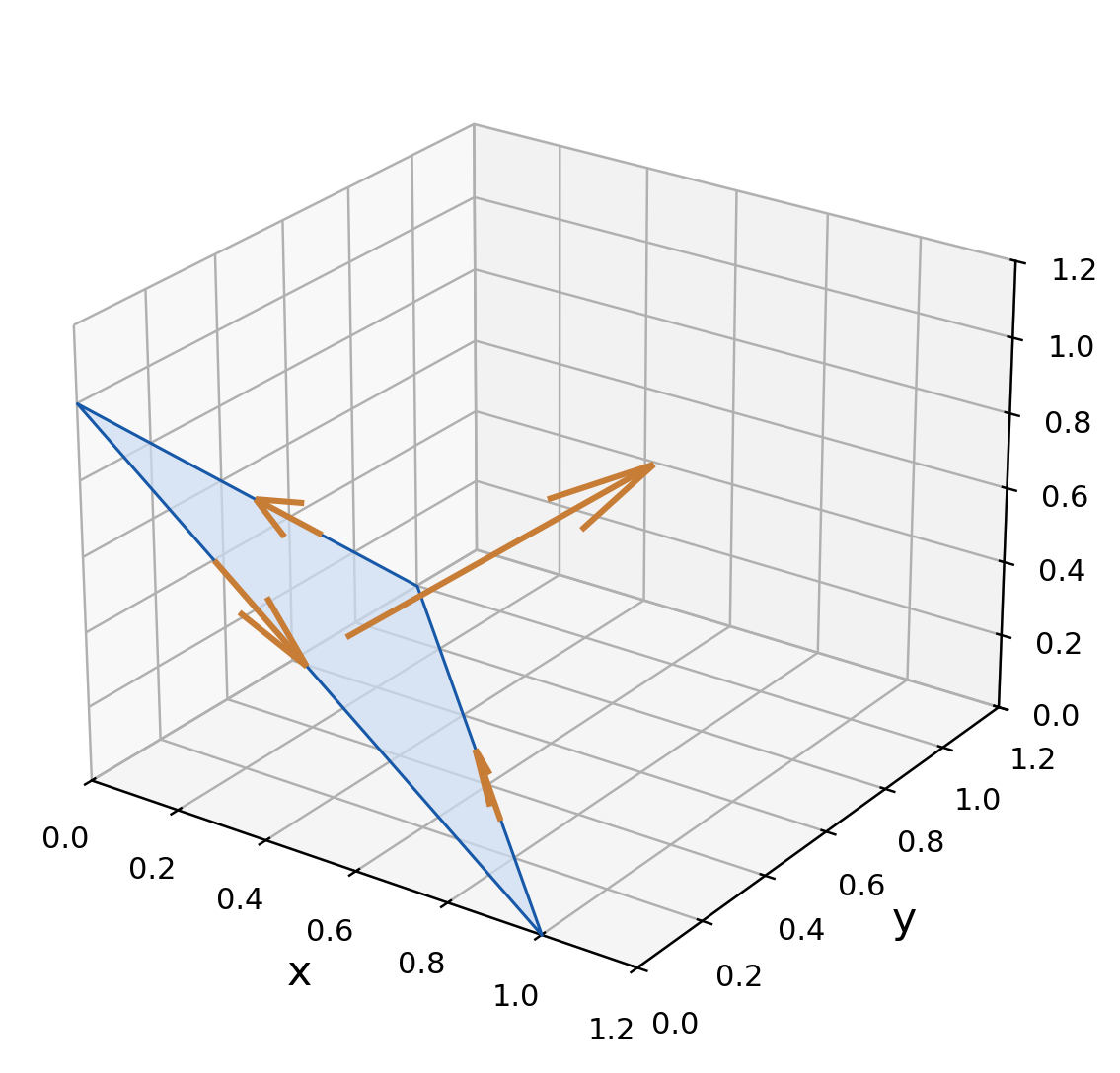
Check with Three Segments
On A→B, use r(t)=(t,0,1−t), 0≤t≤1. Then F=(1−t,t,0), and the dot product with r′=(1,0,−1) is 1−t. This contributes 1/2.
On B→C₀, use r(t)=(1−t,t,0). Then F=(0,1−t,t), and r′=(−1,1,0). The dot product is again 1−t, contributing 1/2.
On C₀→A, use r(t)=(0,1−t,t). Then F=(t,0,1−t), and r′=(0,−1,1). This also contributes 1/2.
W = 1/2+1/2+1/2 = 3/2.
Why the Vector-Area Method Helps
The cross product includes both tilt and area. Using only the unit normal with dx dy would omit the sloping surface’s area factor. Using the nonunit normal with the full sloping dS would count it twice.
Slanted-Plane Method
Express the surface as a graph, calculate its oriented vector area, and integrate over the projected region. State the normal so the boundary sign is unambiguous.
Adding a Gradient Changes No Circulation
Replace F by F+∇ψ, where ψ is smooth near the triangle. Curl(∇ψ)=0, so the Stokes surface integrand is unchanged.
The direct boundary contribution of ∇ψ is also zero because the curve is closed. For ψ=xy, the added field is (y,x,0). Both approaches therefore keep the circulation equal to 3/2.
37. Replacing a Curved Surface
Worked Example 3.106 – Curl Flux Through a Hemisphere
Let F=(−y,x,z), and let S be the upper hemisphere x²+y²+z²=a², z≥0, with outward orientation.
The boundary is the equatorial circle. The outward normal on the upper hemisphere induces anticlockwise traversal viewed from +z.
∇×F = (0,0,2).
Replace the hemisphere by the upward equatorial disk. Both surfaces share the same oriented boundary and the field is smooth everywhere:
∬_S (∇×F)·n dS = 2πa².

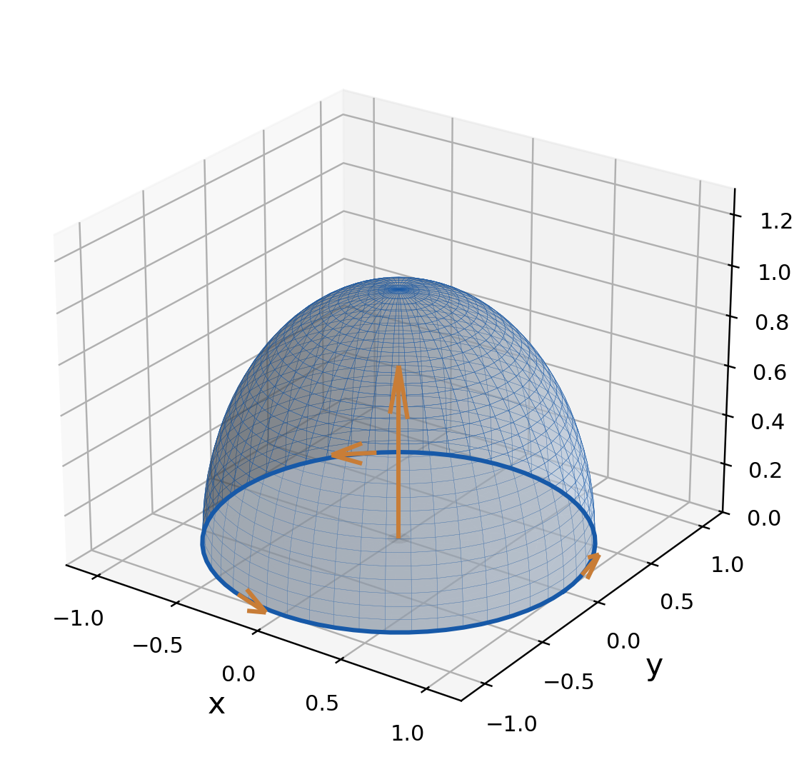
Direct Verification and Signs
On the upper hemisphere, parameterise by polar angle φ from +z and azimuth θ. The outward normal has k-component cos φ, and dS=a²sin φ dφ dθ.
I = ∫[0,2π] ∫[0,π/2] 2a² cos φ sin φ dφ dθ.
I = 2πa².
This confirms the disk replacement.
Closing the Hemisphere
If forming a closed upper half-ball, its bottom disk has downward outward normal, not upward. The bottom curl flux is −2πa², which cancels the hemisphere flux.
That cancellation is consistent with div(curl F)=0. The upward replacement disk used in Stokes and the downward closing disk used for a closed solid have opposite orientations for different purposes.
Surface Replacement Conditions
The field must be smooth on suitable open neighbourhoods of the selected surfaces. A simpler surface that crosses a singularity may be inadmissible even if it shares the boundary.
Sign Distinction
A spanning disk with matched boundary orientation and a closing disk with outward solid orientation can be the same geometric disk with opposite normals.
38. Stokes Orientation and Boundaries
For a surface with several boundary components, the positively oriented boundary integral adds all components with their induced directions. For an upward annulus, the outer boundary is anticlockwise and the inner one clockwise viewed from +z.
Worked Example 3.107 – An Annular Surface
Take F=(−y,x,0) and the annulus 1≤x²+y²≤4 in z=0. Its upward curl flux is:
I = 2π(2²−1²) = 6π.
Directly, the outer circle contributes 8π and the clockwise inner circle contributes −2π:
∮_(∂S) F·dr = 8π−2π = 6π.


Mistake: Integrate F Through the Surface
Stokes uses the normal component of curl F, not the normal component of F itself. Flux of F is a different quantity.
Mistake: Reverse Only the Normal
If the normal is reversed while the boundary traversal stays fixed, the two sides acquire inconsistent signs. Reverse both or insert the corresponding minus sign deliberately.
Mistake: Use a Surface Across a Singularity
A curl-free field around a missing axis can have nonzero circulation. The spanning disk crosses the excluded axis, so the field fails the smoothness hypothesis there.
A Theorem-Selection Check
If a problem gives a closed curve and asks for circulation, Stokes may convert it into a simpler surface integral. If it gives a curl flux through an open surface, Stokes may reduce it to a simpler boundary integral.
Orientation Audit
Draw one normal arrow and one boundary arrow before calculation. For multiple boundary components, draw an arrow on each component rather than assuming all turn the same way.
39. Gauss’ Divergence Theorem
Let E be a solid with a closed piecewise smooth boundary S, oriented outward. Suppose F has continuous first partial derivatives on an open region containing E. Then:
∬_S F·n dS = ∭_E ∇·F dV.
The theorem converts total outward flux through the closed boundary into a volume integral of divergence. It is stated and applied here without proof.

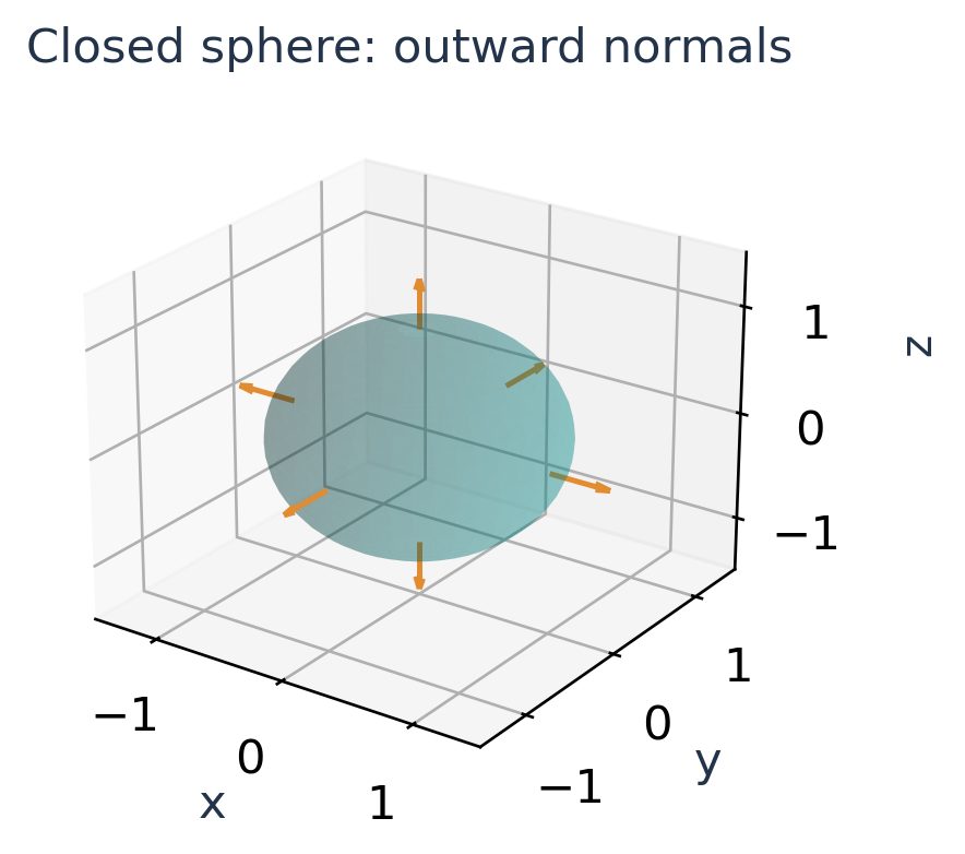

The theorem requires a closed surface. An isolated cap, disk or cylinder side does not enclose a solid by itself.
Worked Example 3.108 – A Constant Field
For a constant vector F=(a,b,c), every spatial derivative is zero. Hence its net outward flux through any closed boundary meeting the theorem’s conditions is zero.
Individual faces or patches can still have positive and negative flux. The theorem adds them over the complete boundary; it does not say the constant field is tangent everywhere.
How to Apply Gauss’ Theorem
- Step 1: Identify the enclosed solid and every boundary piece.
- Step 2: Check that the field is smooth on and inside it.
- Step 3: Calculate the scalar divergence.
- Step 4: Choose convenient volume coordinates and bounds.
- Step 5: Integrate divergence with the correct volume element.
- Step 6: Reverse the result if inward flux was requested.
Worked Example 3.109 – Radial Field Through a Sphere
For F=(x,y,z), div F=3. A radius-a ball has volume 4πa³/3:
Φ = 3(4πa³/3) = 4πa³.
The direct sphere calculation gave the same answer.
Net Flux, Not Total Absolute Crossing
Positive and negative local contributions can cancel. The theorem gives the signed net outward flux, not the integral of |F·n| and not the amount crossing in both directions counted positively.
Singularity Warning
A field undefined at an interior point fails the ordinary smoothness hypothesis. Zero divergence away from that point is not enough to conclude zero flux through a surface enclosing it.
Gauss Checklist
Closed boundary, outward normal, smooth interior, scalar divergence, volume measure. Verify all five before using the shortcut.
40. Gauss’ Theorem on Spheres
Worked Example 3.110 – A Cubic Field
Let F=(x³,y³,z³) and S be the outward sphere r=a. Its divergence is:
∇·F = 3x²+3y²+3z² = 3r².
Use spherical coordinates inside the ball. The volume element contributes r²sin φ:
Φ = 3∫[0,2π] ∫[0,π] ∫[0,a] r⁴ sin φ dr dφ dθ.
Φ = 12πa⁵/5.
The fifth power of a is consistent with a cubic field multiplied by an area scale a².


Worked Example 3.111 – A Diagonal Linear Field
For F=(ax,by,cz) through the radius-R sphere:
Φ = (a+b+c)(4πR³/3).
The constants a,b,c may be positive, negative or zero. Their sum determines the net flux.
Worked Example 3.112 – Zero Net Flux
For F=(x,−y,0), divergence is zero everywhere. Its outward flux through any closed boundary satisfying the theorem’s hypotheses is zero.
The field is not tangent to every such boundary. Some parts can have outward flux and others inward flux; the theorem concerns their signed total.
Inward Orientation
For the cubic field, inward flux is −12πa⁵/5. Do not change the sign of the divergence itself; it is a property of the field. The sign reversal comes from the requested surface orientation.
Direct Versus Theorem Methods
A direct sphere integral requires the normal vector and surface-area element. The theorem replaces those with a scalar divergence and volume element. Choose the shorter calculation while preserving the same physical flux.
Scale Check
For a field homogeneous of degree m, flux through a scaled sphere often scales as radius^(m+2). This provides a useful check before evaluating constants.
41. Gauss’ Theorem on a Cube
Worked Example 3.113 – Quadratic Components
Let F=(x²,y²,z²) on the unit cube 0≤x,y,z≤1. The field is smooth and the cube boundary is closed.
∇·F = 2x+2y+2z.
Φ = ∫[0,1] ∫[0,1] ∫[0,1] (2x+2y+2z) dz dy dx = 3.
Each term contributes 1. The result is positive because all nonzero face contributions point outward.


Worked Example 3.114 – A Centred Cube
For F=(x²,y²,z²) on −1≤x,y,z≤1, the divergence 2(x+y+z) is odd under reflection, so the total outward flux is zero.
Directly, each opposite face pair cancels: x=1 gives positive flux while x=−1 gives negative flux because its outward normal is −i. Squaring the component does not remove the normal’s sign.
Check Face by Face
On x=1, the outward normal is i and F·n=1, giving flux 1. On x=0, the outward normal is −i but F’s x-component is zero, giving flux 0.
The y and z pairs behave identically. Summing six faces gives 1+0+1+0+1+0=3.
Worked Example 3.115 – Mixed Components
For F=(xy,yz,zx) on the same cube:
∇·F = y+z+x.
Φ = 1/2+1/2+1/2 = 3/2.
Directly, x=1 contributes the integral of y over the unit yz-face, giving 1/2; y=1 contributes the integral of z, also 1/2; z=1 contributes the integral of x, again 1/2. The opposite faces contribute zero.
Shifted Boxes
The divergence calculation can be reused for a box with different bounds, but the volume integral changes. Symmetry shortcuts for a centred box need not apply to a box entirely in the positive octant.
Face Check
The normal on a lower coordinate face is negative. Write it explicitly before deciding whether a field component gives positive or negative flux.
42. Gauss on a Cylinder
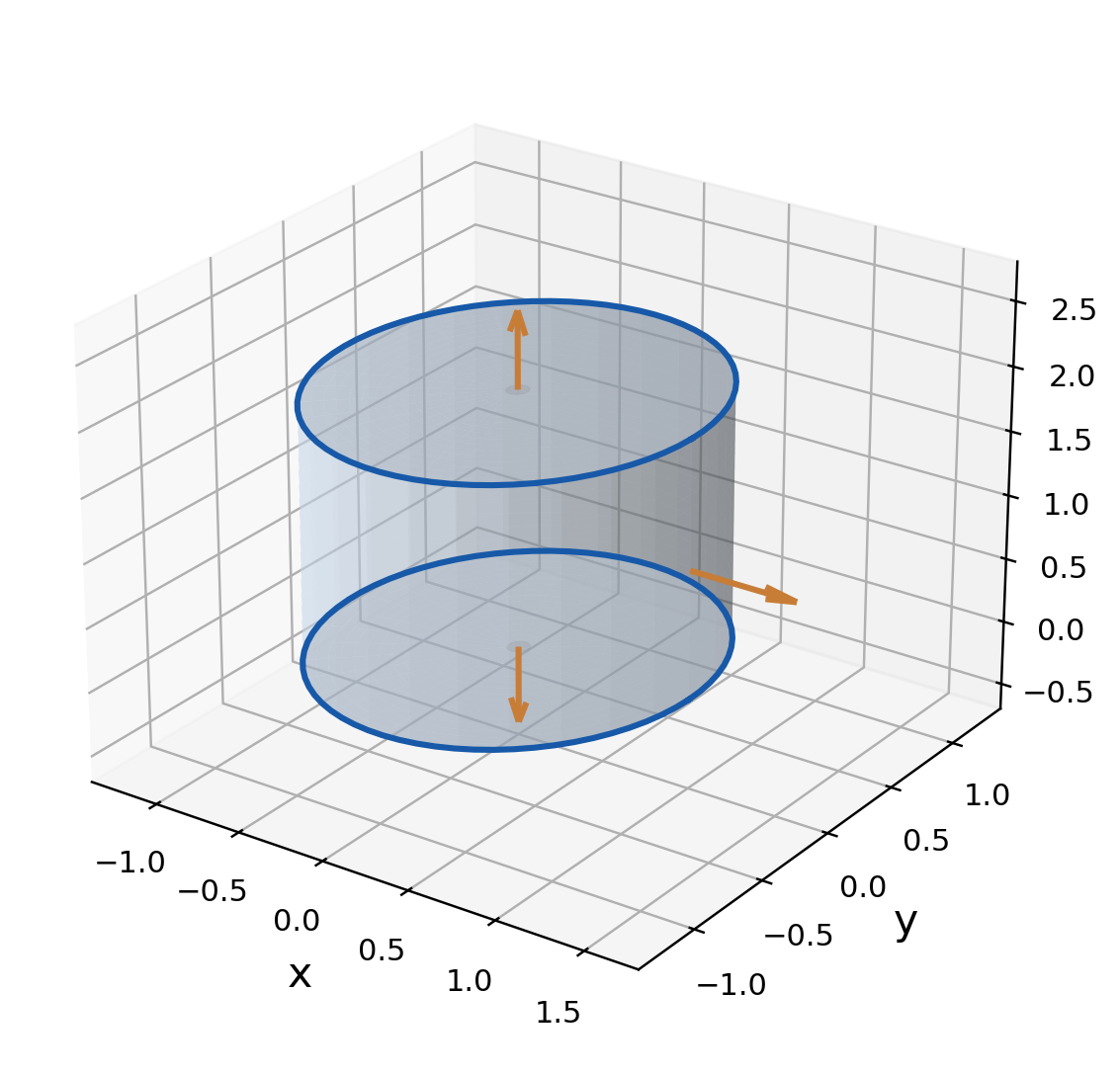
Worked Example 3.116 – A Quadratic Vertical Component
Let F=(x,y,z²), and let E be the cylinder r≤a, 0≤z≤h. Then:
∇·F = 2+2z.
Use cylindrical coordinates:
Φ = ∫[0,2π] ∫[0,a] ∫[0,h] (2+2z)r dz dr dθ.
Φ = πa²(2h+h²).
The radial factor r comes from the volume element, not from the divergence. Forgetting it would produce the wrong dependence on a.

Direct Verification
On the side, the outward normal is horizontal. The dot product with (x,y,z²) is a, so the side flux is 2πa²h.
On the top, z=h and n=k, giving flux h²πa². On the bottom, z=0 and n=−k; the vertical component is zero.
Φ = 2πa²h+πa²h².
This agrees with the divergence theorem.
Worked Example 3.117 – Flux Through Only the Side
If the question asks for the curved side alone, subtract the top and bottom fluxes from the closed-surface result. Here that leaves 2πa²h.
The closed-surface theorem does not automatically equal the side flux just because the solid is described as a cylinder.
A Translating Cylinder
If the lower and upper z-levels are z₀ and z₁, integrate 2+2z over that interval. The bottom contribution is then generally nonzero and has negative outward normal.
Closure Strategy
Use “closed total minus added faces” for open surfaces. State which normals belong to the closed solid so the subtraction signs remain consistent.
43. Gauss on a Tetrahedron
Worked Example 3.118 – First-Octant Tetrahedron
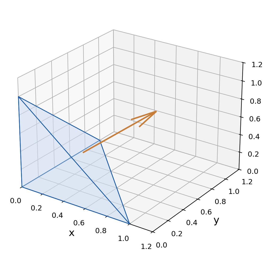
Let E={x,y,z≥0,x+y+z≤1} and F=(x,y,z). Its volume is 1/6 and div F=3, so:
Φ = 3(1/6) = 1/2.
Only the sloping face contributes to direct outward flux. On x=0,y=0,z=0, the matching field component is zero.
For the sloping face z=1−x−y, the outward vector area is (1,1,1)dx dy. The dot product is x+y+z=1. Its triangular projection has area 1/2, giving the same answer.

Worked Example 3.119 – A Single Vertical Component
For F=(0,0,z) on the unit tetrahedron, divergence is 1:
Φ = ∭_E 1 dV = 1/6.
On the sloping face the direct flux density is z=1−x−y. Its integral over the unit triangle is also 1/6. All coordinate-plane face contributions vanish for this field.
Worked Example 3.120 – Quadratic Field
For F=(x²,y²,z²), divergence is 2(x+y+z). Over the unit tetrahedron, the integrals of x,y,z are each 1/24:
Φ = 2(1/24+1/24+1/24) = 1/4.
Bounds Written Fully
The volume integral can be written:
Φ = ∫[0,1] ∫[0,1−x] ∫[0,1−x−y] 2(x+y+z) dz dy dx.
The outer projection is the same triangle used in the direct sloping-face calculation, but the measures differ: a volume integral includes dz, while the face integral uses oriented area.
Worked Example 3.121 – Scale the Tetrahedron
For x+y+z≤a with a>0 and F=(x,y,z), divergence remains 3 and volume becomes a³/6. Hence flux is a³/2.
For the quadratic field, scaling contributes a⁴, so its flux is a⁴/4.
Compare Methods
Coordinate-plane faces may vanish in a direct flux calculation, while a constant divergence may make the volume method even shorter. Check both possibilities before choosing.
44. Choosing the Correct Integral Theorem
| Given Quantity | Useful Method |
|---|---|
| Work from A to B in a gradient field | Potential difference |
| Circulation around a closed curve | Stokes’ theorem |
| Curl flux through an open surface | Stokes via its boundary |
| Flux of F through a closed surface | Gauss’ divergence theorem |
| Scalar mass of a wire | Scalar line integral |
| Scalar surface area or surface mass | Scalar surface integral |
Stokes relates a boundary curve to an oriented surface. Gauss relates a closed surface to an enclosed volume. Neither theorem is a substitute for identifying the requested quantity.
Worked Example 3.122 – Select Without Calculating
For ∮_C F·dr around a circle, inspect curl and a spanning disk. For outward flux of F through a sphere, inspect divergence and the enclosed ball.
Worked Example 3.123 – The Same Field and Sphere
Let F=(x,y,z), S be a radius-a sphere and C its equatorial circle.
The closed-surface flux of F is 4πa³. The circulation of F around C is zero because F is conservative, with potential r²/2.
The curl flux through any admissible surface bounded by C is also zero because curl F=0.
These are three distinct quantities. A nonzero flux of F does not imply nonzero circulation of F.
Assumption Checklist
For Stokes, check smoothness near the chosen surface and pair its normal with the boundary direction. For Gauss, check smoothness on and inside the solid and use the outward closed boundary.
For a potential shortcut, verify a differentiable potential on a region containing the path. A singularity cannot be ignored merely because it occupies a small set.
A Sign Habit
Write “upward,” “downward,” “outward” or “inward” next to the selected normal. Write the curve’s viewing direction next to “clockwise” or “anticlockwise.”
Method Selection
Choose the theorem from the integral’s meaning and geometry, then examine which side is easier to evaluate. Do not choose only because one derivative happens to be zero.
45. AI Heat Maps as Scalar Fields
A heat map represents a scalar value over a coordinate domain. In an AI context the value might be a model score, loss or spatial intensity. A mathematical heat map does not automatically represent physical temperature or causal importance.
The gradient identifies the local direction of fastest increase in the specified scalar field. Contours connect points with equal values.


Worked Example 3.124 – Gaussian Score Field
Let H=e^(−x²−y²). Then:
∇H = −2e^(−(x²+y²))(x,y).
At (1,0), the gradient is (−2/e,0). The score increases most rapidly toward decreasing x, with maximum local rate 2/e.
Worked Example 3.125 – A Chosen Direction
At (1,0), choose u=(1,1)/√2. Then:
DᵤH = −√2/e.
The negative sign means this diagonal direction initially lowers the score. The opposite unit direction gives the positive rate √2/e.
Finite Differences in a Sampled Map
For an interior grid point with spacing h, a central difference approximates the x-derivative:
Hₓ(x,y) ≈ [H(x+h,y)−H(x−h,y)]/(2h).
Use the corresponding y-difference for Hᵧ. The formula assumes enough smoothness and access to both neighbours; edges need another rule or boundary padding.
Worked Example 3.126 – Exact Quadratic Difference
For S=x²+2y², the central x-difference at (1,1) is exactly 2 for any nonzero h in exact arithmetic. The y-difference is exactly 4. Higher-order smooth fields generally have truncation error.
Interpretation
A gradient describes local sensitivity of the stated field in the stated coordinates. It does not by itself prove why a trained model made a prediction.
46. Gradient Steps in a Model Loss
A model loss depending on several parameters is a scalar field in parameter space. Gradient descent takes a step opposite the gradient:
w_new = w−α∇L(w), α>0.
For a sufficiently small step at a nonstationary point of a smooth loss, the first-order change is negative. A large step can overshoot and increase the loss.
Worked Example 3.127 – A Fully Specified Quadratic
Let L=(w₁−2)²+2(w₂+1)². Its gradient is:
∇L = (2(w₁−2),4(w₂+1)).
At w=(0,0), L=6 and ∇L=(−4,4). With α=0.1, the next point is (0.4,−0.4).
L_new = 1.6²+2(0.6)² = 3.28.
Worked Example 3.128 – Overshooting
For the same start but α=1, the next point is (4,−4). Its loss is:
L = 2²+2(−3)² = 22.
The direction was downhill locally, but the finite step increased the loss. The gradient alone does not guarantee improvement for an arbitrary step size.


First-Order Estimate
At the start, |∇L|²=32. A step −α∇L has estimated loss change −32α. For α=0.1 this predicts −3.2, while the exact change is −2.72; the discrepancy comes from second-order terms.
Scaling Coordinates
Different parameter units can strongly change gradient components and contour shapes. A steep component does not automatically mean that parameter is more intrinsically important; its numerical scale matters.
Model Scope
This example illustrates vector-calculus reasoning on a stated quadratic. It is not a training result from a neural network or evidence of performance on a dataset.
47. Robotics: Velocity and Path Direction
A planned robot position r(t) defines a path and a time law. Its derivative gives velocity, its magnitude gives speed, and the normalised velocity gives the instantaneous direction of travel.
A vector field can provide desired local motion directions, but an actual robot also has speed, acceleration, obstacle and actuator constraints.
Worked Example 3.129 – A Planar Planned Path
Let r(t)=(t,t²), 0≤t≤1. Then:
v = (1,2t), a = (0,2).
At t=1/2, velocity is (1,1), speed is √2 and the unit travel direction is (1,1)/√2.

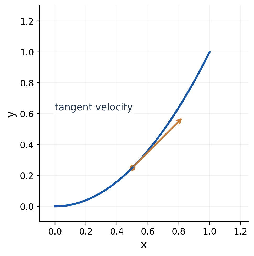
Worked Example 3.130 – Spatial Cost per Distance
Suppose cost density is c(x,y)=x along this path. Then total distance-weighted cost is:
I = ∫[0,1] t√(1+4t²) dt = (5√5−1)/12.
This uses ds and is independent of how fast the same geometric path is traversed under this purely spatial cost model.
Work-Like Cost Differs
If a resistance field F is specified, the mechanical work model uses ∫F·dr instead. If a time penalty is specified, the cost may use ∫c(r(t),t)dt. These are different models and should not be mixed.
Worked Example 3.131 – Tracking a Desired Direction
At (1,1), let the desired field be F=(2−x,−y)=(1,−1). Its unit direction is (1,−1)/√2. A commanded speed v₀ would give velocity v₀F/|F|, provided F≠0.
At a zero of the field, normalisation is undefined and a stopping or fallback rule is needed.
Robotics Interpretation
A geometric direction field does not automatically provide a safe time-parameterised trajectory. Distinguish direction, speed, acceleration and accumulated cost.
48. Robotics: Potential Fields
An attractive potential can guide motion toward a goal. For goal g and position p in a plane, use U_att=|p−g|²/2. Then −∇U_att points toward the goal.
Worked Example 3.132 – Attractive Direction
Let g=(2,0) and p=(0,1). The gradient of U_att is p−g=(−2,1), so the attractive direction is (2,−1).
A model obstacle at o may be represented away from o by a repulsive potential:
U_rep = k/(2|p−o|²), k>0.
−∇U_rep = k(p−o)/|p−o|⁴.
The field points away from the obstacle but becomes singular at its centre.

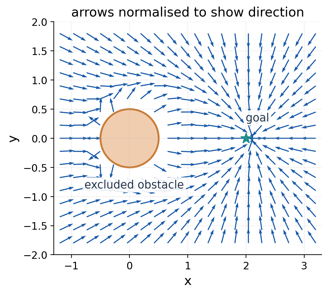
Worked Example 3.133 – Total Direction at a Point
Take k=1, o=(0,0), g=(2,0), p=(0,1). The repulsive vector is (0,1), while the attractive vector is (2,−1). Their sum is (2,0).
This is only the local field value at that point. It does not prove the entire resulting path reaches the goal or avoids all obstacles.
Local Minima Can Trap Motion
A combined potential can have stationary points away from the goal. At such a point, the negative gradient is zero and simple gradient-following can stop.
A practical planner may need global search, a navigation function, recovery behaviour or explicit collision checking. Those engineering choices go beyond calculating a gradient.
Domain and Finite Robot Size
A point-obstacle singularity is a mathematical simplification. A real robot has size, so the forbidden region should account for the robot footprint and safety clearance rather than excluding only the centre point.
Work Interpretation
For a smooth potential on an admissible path, the work of −∇U is U(start)−U(end). A path crossing a singular obstacle is outside the model’s valid domain.
Model Limitation
Potential fields explain local guidance but do not guarantee a globally safe or complete path planner. Keep the excluded obstacle region explicit in the diagram and domain.

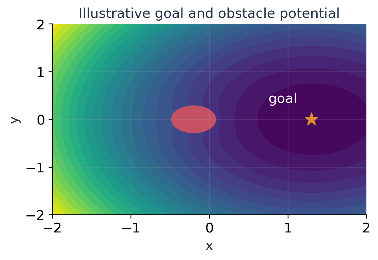
49. Computer Graphics: Surface Normals
Surface normals control geometric orientation and are used in simple lighting models. For an implicit surface φ(x,y,z)=0, a nonzero gradient supplies a normal direction.
For a graph z=g(x,y), an upward normal is (−gₓ,−gᵧ,1). Normalise it before a lighting dot product that assumes a unit normal.
Worked Example 3.134 – A Paraboloid Normal
For z=x²+y² at (1,0,1), the upward normal is (−2,0,1). Its magnitude is √5:
n̂ = (−2,0,1)/√5.
The downward normal is its negative. The choice affects the illuminated side of a surface.

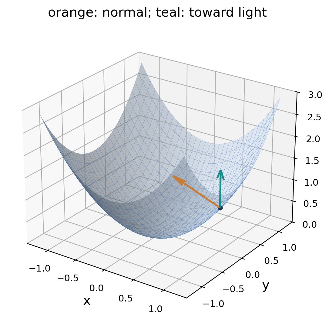
A Simple Diffuse-Lighting Model
Suppose the unit vector l points from the surface toward a light source. A simple diffuse factor is:
I = max(0,n̂·l).
This is a stated simplified model, not a full rendering equation. Material colour, shadows, distance effects and specular reflection are not included here.
Worked Example 3.135 – Vertical Light
With l=(0,0,1), the paraboloid normal gives I=1/√5. Using the unnormalised normal would give 1 instead and lose the tilt effect.
Worked Example 3.136 – Light from Below
With l=(0,0,−1), the dot product is −1/√5, so the clamped factor is zero. The chosen upward-facing side receives no direct diffuse contribution in this model.
Triangle-Mesh Normal
For triangle vertices A,B,C, use (B−A)×(C−A). Reversing the vertex order reverses the normal. A zero cross product indicates a degenerate triangle and cannot be normalised.
Graphics Check
State whether the light vector points toward or away from the light and keep the normal’s orientation consistent with the face winding order.

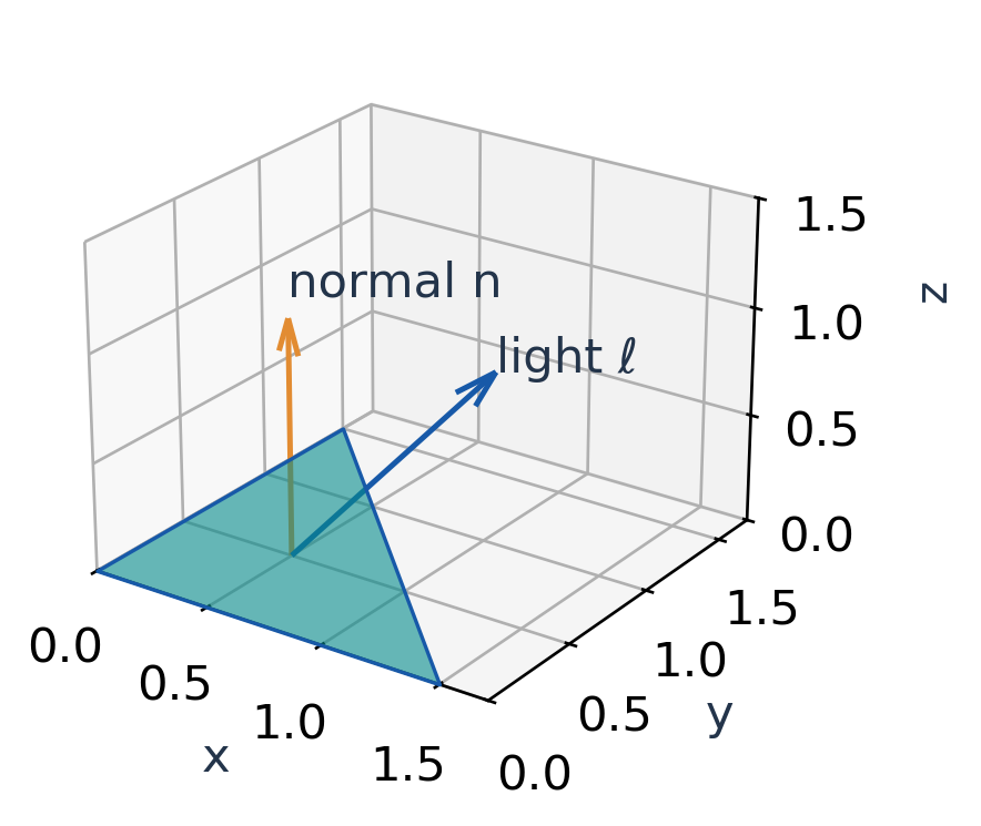
50. Computer Graphics: Vector Fields
Vector fields can describe local motion in particle animations or flow visualisations. Divergence indicates local expansion or compression; curl indicates local rotational behaviour.
These quantities help distinguish fields that look similar in a sparse arrow plot. Numerical integration is then needed to move particles through time.
Worked Example 3.137 – A Rotational Animation Field
Let F=(−y,x). Its planar divergence is zero and its k-curl component is 2. Exact trajectories satisfy x²+y²=constant.
The radius stays constant because:
d(x²+y²)/dt = 2x(−y)+2y(x) = 0.

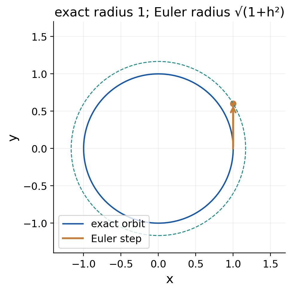
Worked Example 3.138 – One Forward-Euler Step
For step size h>0:
x_new = x−hy, y_new = y+hx.
Then:
x_new²+y_new² = (1+h²)(x²+y²).
Thus forward Euler increases radius for any nonzero h at a nonzero point, even though the exact continuous field preserves radius. The numerical method and continuous vector field are different layers of the model.
Worked Example 3.139 – Expansion Field
For F=(x,y), divergence is 2 and curl is zero. Exact trajectories move radially with r(t)=r(0)eᵗ. An initially small area expands as e^(2t), consistent with the divergence.
Sampling Caution
A pixel-grid field estimates spatial derivatives from neighbouring values. Coarse resolution can hide sharp changes; boundaries need defined rules. A smooth analytic field and a sampled approximation need not produce identical derivative estimates.
Interpretation
A visible numerical spiral may come from the time integrator rather than from the intended continuous field. Check invariants such as radius before changing the field itself.

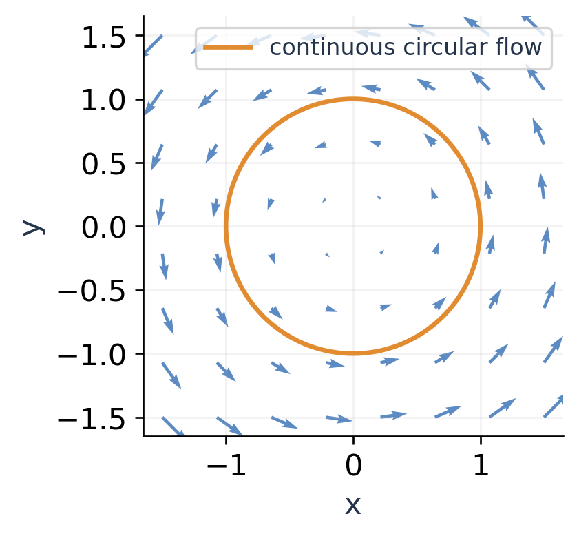
51. Mixed Solved Revision
Worked Example 3.140 – Gradient and Unit Direction
For φ=x²+y²+z² at (1,2,2), ∇φ=(2,4,4) with magnitude 6. In direction a=(1,0,1), the unit vector is (1,0,1)/√2:
Dᵤφ = (2+4)/√2 = 3√2.
This is smaller than the maximum rate 6, as expected.
Worked Example 3.141 – Solenoidal Parameter
Let F=(kx,−2y,3z). Divergence is k−2+3=k+1. The field is solenoidal when k=−1.
Worked Example 3.142 – Potential Difference
For F=(yz,xz,xy)=∇(xyz), work from (1,1,1) to (2,1,3) is:
W = 6−1 = 5.
Worked Example 3.143 – Local Values of Both Operators
For F=(xy,yz,zx), evaluate at (1,1,1):
∇·F = 3, ∇×F = (−1,−1,−1).
The field value at that point is (1,1,1). Field, divergence and curl have different meanings even when some numerical components happen to match in magnitude.
Worked Example 3.144 – Stokes on a Square
For F=(−y,x,0), take the boundary of 0≤x≤2, 0≤y≤1 in z=0, anticlockwise from +z. Curl·k=2 and area=2:
∮_C F·dr = 4.
Worked Example 3.145 – Gauss on a Box
For F=(x,y,z), take 0≤x≤2, 0≤y≤1, 0≤z≤3. Divergence is 3 and volume is 6:
Φ = 3×6 = 18.
Worked Example 3.146 – Direct Graph Flux
For F=(0,0,1) through z=x+y over the unit square with upward orientation, use vector area (−1,−1,1)dx dy. The dot product is 1, so flux is 1, not the sloping area √3.
Final Comparison
The Stokes example uses curl over an oriented surface. The Gauss example uses divergence over a volume. The direct graph example uses the original field dotted with vector area. Naming the integral type first keeps these methods distinct.
Revision Habit
For every answer, give the chosen direction or normal and one check on sign, scale or magnitude. A correct number without a valid orientation can still answer the wrong question.
Worked Example 3.147 – A Wire Integral Check
On a radius-2 circle, the scalar field f=x²+y² equals 4. Its arc-length integral is:
∫_C f ds = 4(4π) = 16π.
This remains positive in either traversal direction. Compare with a rotational-field circulation, whose sign reverses when the curve direction is reversed.
52. Short-Answer Checks with Answers
What Is a Scalar Point Function?
It assigns one scalar value to every allowed point, such as temperature or density. A vector point function assigns a vector instead.
What Does the Gradient Represent?
At a differentiable point with nonzero gradient, it points toward the strongest first-order increase of the scalar field. Its magnitude is the maximum directional derivative.
Why Normalise a Direction Vector?
The directional derivative is a rate per unit distance. Using a nonunit vector scales the result by its magnitude and instead measures change per unit parameter along that displacement.
What Is a Solenoidal Field?
A C¹ vector field with divergence identically zero on its domain. This does not imply the field itself is zero or that its curl vanishes.
What Is an Irrotational Field?
A C¹ vector field with curl identically zero on its domain. A global potential also needs appropriate domain conditions.
Is Zero Curl Always Enough for a Potential?
No. On an open simply connected domain, a C¹ curl-free field has a global potential. A domain with an excluded axis can support nonzero closed circulation despite zero local curl.
What Changes Under Path Reversal?
A work integral ∫F·dr changes sign. A scalar arc-length integral ∫f ds does not, because ds is nonnegative length.
What Does Stokes’ Theorem Equate?
Circulation of F around an oriented boundary curve and normal flux of curl F through a spanning oriented surface, with the required smoothness and paired orientation.
What Does Gauss’ Theorem Require?
A closed piecewise smooth outward boundary and a C¹ field on an open region containing the solid. It equates total outward flux of F with the volume integral of div F.
Can Zero Net Flux Hide Local Crossing?
Yes. Outward and inward contributions can cancel. Zero net flux does not mean the field is tangent at every surface point.
Why Is a Graph’s Vector Area Useful?
For upward z=g(x,y), it is (−gₓ,−gᵧ,1)dx dy, combining normal orientation and surface-area scale in one expression.
Answer Standard
State the mathematical condition and interpretation together. Avoid replacing a theorem’s hypotheses with a visual guess about the arrows.
53. Formula Sheet
For F=(P,Q,R) in Cartesian coordinates:
∇φ = (φₓ,φᵧ,φ_z).
Dᵤφ = ∇φ·u, |u|=1.
∇·F = Pₓ+Qᵧ+R_z.
∇×F = (Rᵧ−Q_z,P_z−Rₓ,Qₓ−Pᵧ).
∇²φ = φₓₓ+φᵧᵧ+φ_zz.
Smooth-Field Identities
∇×∇φ = 0.
∇·(∇×F) = 0.
The mixed-derivative identities use sufficient second-order smoothness.
Curve Elements
dr = r′(t)dt, ds = |r′(t)|dt.
T = r′/|r′|, r′≠0.
The tangent formula needs a regular parameterisation.
Product Rules
∇(φψ) = φ∇ψ+ψ∇φ.
∇·(φF) = ∇φ·F+φ∇·F.
The operator differentiates both factors. A constant multiplier can pass through unchanged; a variable multiplier requires its derivative term. Use parentheses to show the full expression being differentiated.
Integral Formulas
∫_C f ds = ∫[a,b] f(r(t))|r′(t)| dt.
∫_C F·dr = ∫[a,b] F(r(t))·r′(t) dt.
For F=∇φ on a suitable path domain:
∫_C F·dr = φ(B)−φ(A).
For an upward graph z=g(x,y):
dS_vector = (−gₓ,−gᵧ,1) dx dy.
Stokes’ Theorem
∮_(∂S) F·dr = ∬_S (∇×F)·n dS.
Pair surface normal and boundary orientation; require F to be C¹ near the surface.
Gauss’ Divergence Theorem
∬_(∂E) F·n dS = ∭_E ∇·F dV.
Use the outward closed boundary; require F to be C¹ on a neighbourhood of the solid.
Final Self-Check
Normalise directions; distinguish scalar and vector outputs; use dr for work and ds for length; include all faces for a closed surface; check singularities before theorem shortcuts.


