


University: Dr. A.P.J. Abdul Kalam Technical University (AKTU) Programme: B.Tech First Year, Semester I Course Code: AAS103D Stream: CSE Unit: I – Calculus
Unit I Introduction
Calculus of several variables studies quantities controlled by more than one input. A surface, a model loss, a processing cost or a measured volume can change when several inputs change together.
This unit develops limits, continuity, partial derivatives and differentiability before using them in expansions, coordinate changes, optimisation and error approximation. Every formula is connected to its assumptions and a worked method.
Complete Syllabus Map
| Topic | PDF Pages |
|---|---|
| Functions, limits and continuity | 2–9 |
| Partial derivatives and differentiability | 10–17 |
| Composite functions and total derivatives | 18–22 |
| Euler’s homogeneous-function theorem | 23–26 |
| Two-variable expansion | 27–30 |
| Jacobians and their properties | 31–36 |
| Unconstrained extrema | 37–43 |
| Lagrange multipliers | 44–48 |
| Errors and CSE applications | 49–53 |
| Solved revision and formula sheet | 54–56 |
Central Idea
A multivariable limit must control every nearby path. A derivative must describe a valid local change. An optimisation answer must respect the domain and constraints.
How to Use These Notes
- Write the function’s domain before a limit or optimisation problem.
- In a partial derivative, identify which variables stay fixed.
- For composite functions, draw the dependence paths before differentiating.
- Check smoothness assumptions before interchanging mixed derivatives.
- Distinguish a local stationary point from a global optimum.
- Use signed differentials for estimated change and absolute values for first-order worst-case error estimates.
Essential Notation
| Symbol | Meaning |
|---|---|
| fₓ, fᵧ | First partial derivatives |
| fₓᵧ | Differentiate fₓ with respect to y |
| h, k | Small changes in x and y |
| df | First-order differential |
| ∇f | Vector of first partial derivatives |
| H | Hessian of second derivatives |
| J | Jacobian determinant |
| λ | Lagrange multiplier |
Unless stated otherwise, angles in trigonometric derivatives use radians. A displayed model describes the stated mathematical function, not measured cloud or machine-learning performance.
Taylor expansion approximates a function near a chosen input pair. Jacobians organise coordinate changes; stationary-point and multiplier methods use derivatives to solve optimisation problems.
1. Functions of Two Variables
A function f assigns one output to each permitted input pair (x,y). Its domain is a subset of the input plane; its graph consists of points (x,y,f(x,y)) in three-dimensional space.
The same notation can describe temperature depending on position, a cost depending on two resource quantities, or a model error depending on two adjustable parameters. The inputs and units must be identified in each application.
Domain Restrictions
A denominator cannot be zero. A real square root requires a nonnegative radicand. A real logarithm requires a strictly positive argument. Multiple restrictions must hold together.
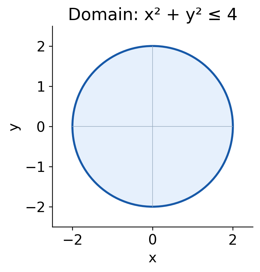
Worked Example 1.1: Find a Real Domain
Consider:
f(x,y) = √(4 − x² − y²)
The square-root condition is:
x² + y² ≤ 4
The domain is the closed disk of radius 2. Boundary points are included because a square root of zero is defined.

Domain, Range and Graph
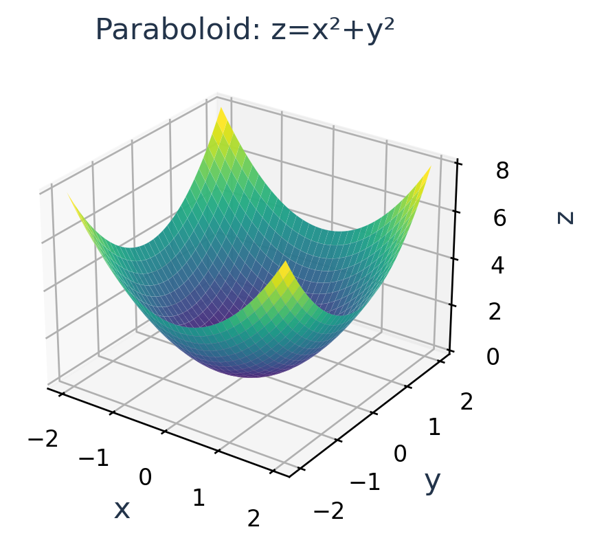
For the same function, the smallest value is 0 on the boundary and the largest is 2 at the origin. Its range is therefore [0,2]. Its graph is the upper hemisphere of a sphere of radius 2.
The disk is the domain; the hemisphere is the graph. Confusing them loses the difference between input points and input–output points.
Worked Example 1.2: Combine Restrictions
Let:
g(x,y) = ln(x+y)/(x−y)
The logarithm requires x+y>0. The denominator requires x≠y. Thus the domain is the open half-plane x+y>0 with the line x=y removed wherever it lies in that half-plane.
The restrictions should not be replaced by x>0 and y>0. A point such as (2,−1) is allowed because its sum is positive and its coordinates are unequal.
Check a Candidate Point
At (2,−1):
g(2,−1) = ln(1)/3 = 0
At (1,1), the denominator is zero. At (−1,−1), the logarithm is not real.
Why Domain Comes First
Limits are taken through points in the domain. A formula simplification may extend a function to a removed point, but it does not silently change the original domain.
Exam Habit: List each restriction, intersect them, then describe or sketch the resulting set. Test one allowed and one excluded point to check your interpretation.

2. Surfaces and Level Curves

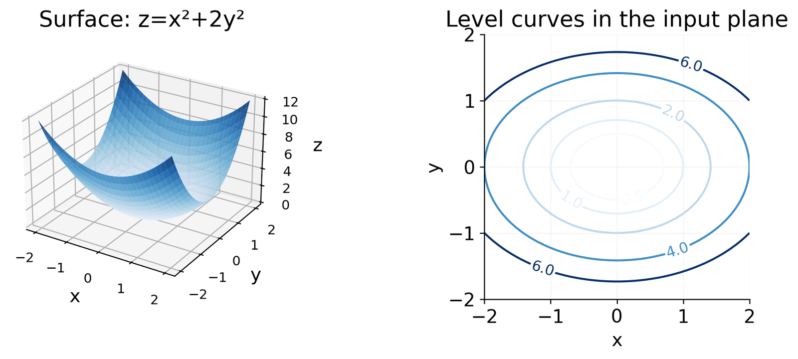
For z=f(x,y), a surface gives height above the input plane. A level curve f(x,y)=c collects inputs that produce one fixed output c.
Worked Example 1.3: Find Level Curves
For f(x,y)=x²+2y², the level equation is:
x² + 2y² = c
If c>0, these are ellipses. If c=0, only the origin remains. If c<0, there are no real level points because both squared terms are nonnegative.
For c=2, the intercepts are x=±√2 and y=±1. Checking intercepts helps label the axes correctly.
Reading a Contour Map
Close spacing between consecutive equally spaced levels can indicate a rapid change of height in the corresponding direction. The interpretation depends on the chosen contour values and scale.
A Slice Is Different
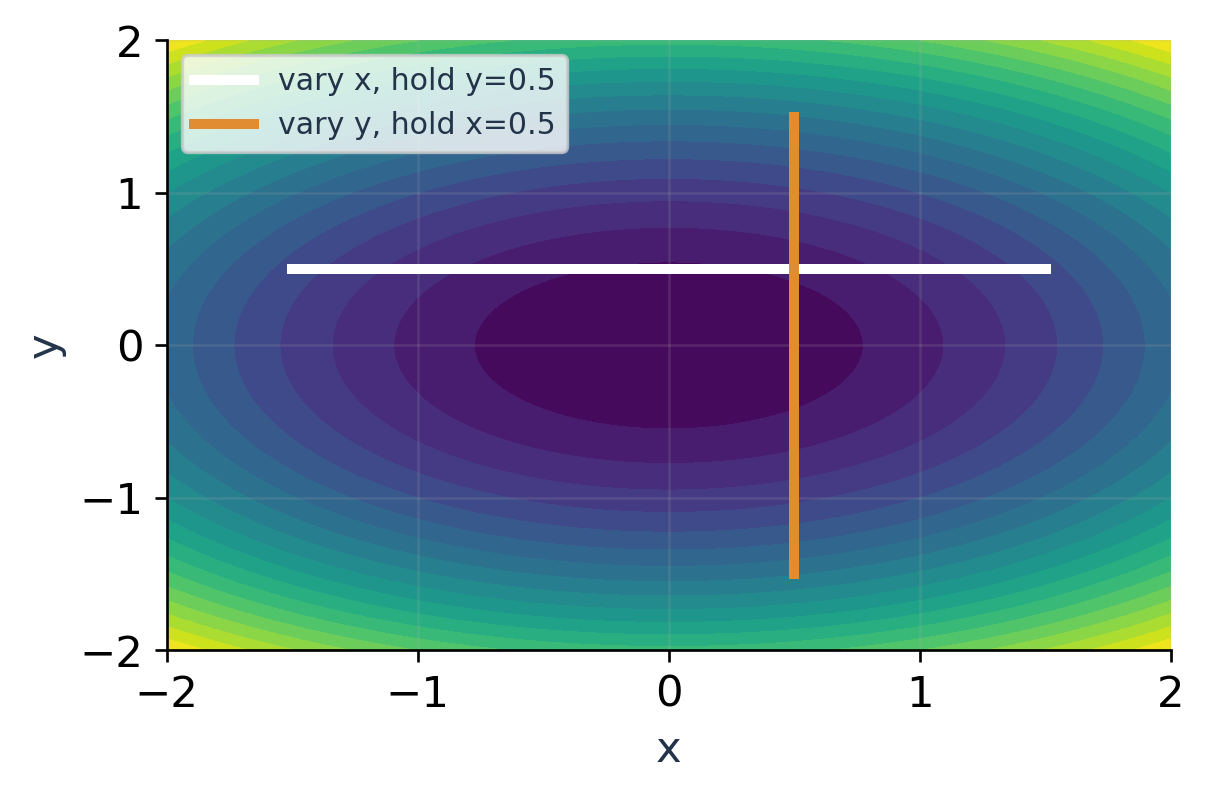
Setting y=1 gives the one-variable slice z=x²+2. Setting x=1 gives z=1+2y². These slices describe coordinate changes and will later define partial slopes.
A level curve instead changes x and y together while keeping z fixed. It should not be used as if one coordinate were held constant.
Application Connection
A loss contour marks parameter combinations with equal model loss. A resource-cost contour marks combinations with equal cost. The mathematical geometry is useful before any optimisation algorithm is introduced.
Quick Interpretation Checks
- Surface axes are x, y and output z.
- A contour plot uses the input x–y plane.
- A contour label is an output value.
- Moving along a contour leaves the function value unchanged.
Visual Rule: A contour plot compresses height into labels. Read the contour values as well as the drawn spacing before concluding that a region is steep or flat.
3. Meaning of a Two-Variable Limit
The statement f(x,y) approaches L as (x,y) approaches (a,b) means that every sufficiently close domain point, except possibly the point itself, gives a value close to L.
lim[(x,y)→(a,b)] f(x,y) = L
A precise formulation uses the distance √[(x−a)²+(y−b)²]. For every ε>0, there must be a δ>0 such that domain points satisfying a positive distance less than δ also satisfy |f(x,y)−L|<ε.


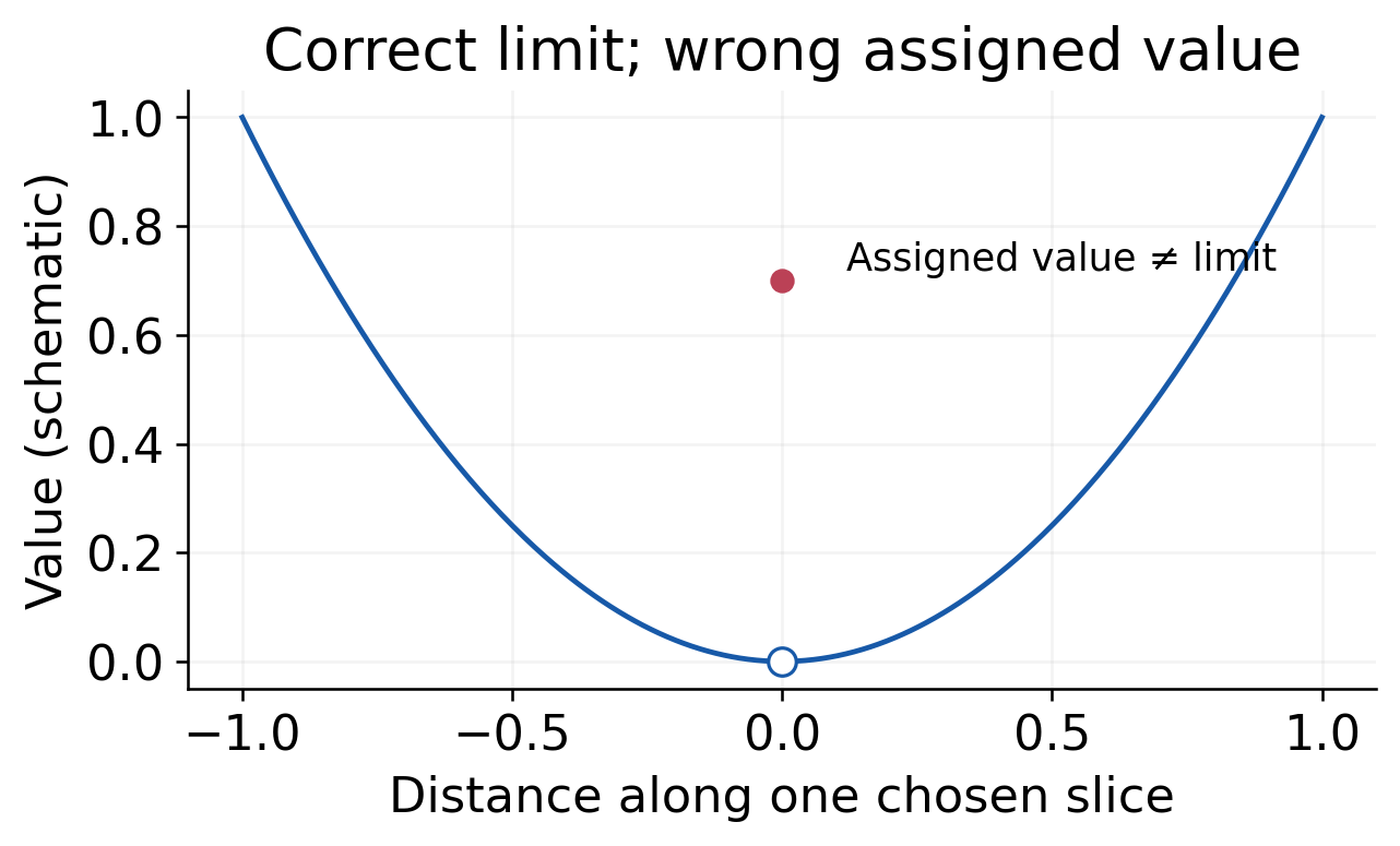
The function need not be defined at (a,b) for its limit there to exist. Its assigned value at the point is not used in the punctured-neighbourhood condition.
Worked Example 1.4: A Direct Limit
Find the limit of x²+xy+2y² as (x,y) approaches (1,2).
Polynomials are continuous everywhere, so direct substitution is valid:
1² + (1)(2) + 2(2²) = 11
The limit is 11.
This is not merely an experimental guess from a table. The polynomial limit laws justify replacing the variables by their limiting values.
Quotient Rule for Limits
If numerator and denominator have limits and the denominator limit is nonzero, the quotient limit is their quotient. If both approach zero, the quotient rule does not settle the problem.
A Useful Strategy
First check the domain and whether ordinary limit laws apply. If substitution creates an indeterminate expression, simplify, compare paths or find a uniform estimate.
Path Independence Is Necessary
If a full limit exists, every allowed path approaching the point has that same limit. Two paths with different limits therefore disprove existence.
The reverse is not established by checking only a few paths. Even all straight lines can miss behaviour along a curved path.
Important Logic: A path test is powerful for disproving a limit. Proving a limit normally requires an argument that controls all nearby domain points.
4. Path Tests: Finding a Contradiction
Different approaches to the same point can produce different outputs. This is the main new obstacle beyond a one-variable limit.


Worked Example 1.5: Two Unequal Line Limits
For f(x,y)=xy/(x²+y²), examine the origin.
Along y=0 with x≠0:
f(x,0) = 0
Along y=x with x≠0:
f(x,x) = x²/(2x²) = 1/2
The two limits differ. Therefore the two-variable limit does not exist.
No choice of the function value at (0,0) can repair this missing limit. Redefining one point cannot remove the disagreement between nearby paths.
A Whole Family of Line Limits
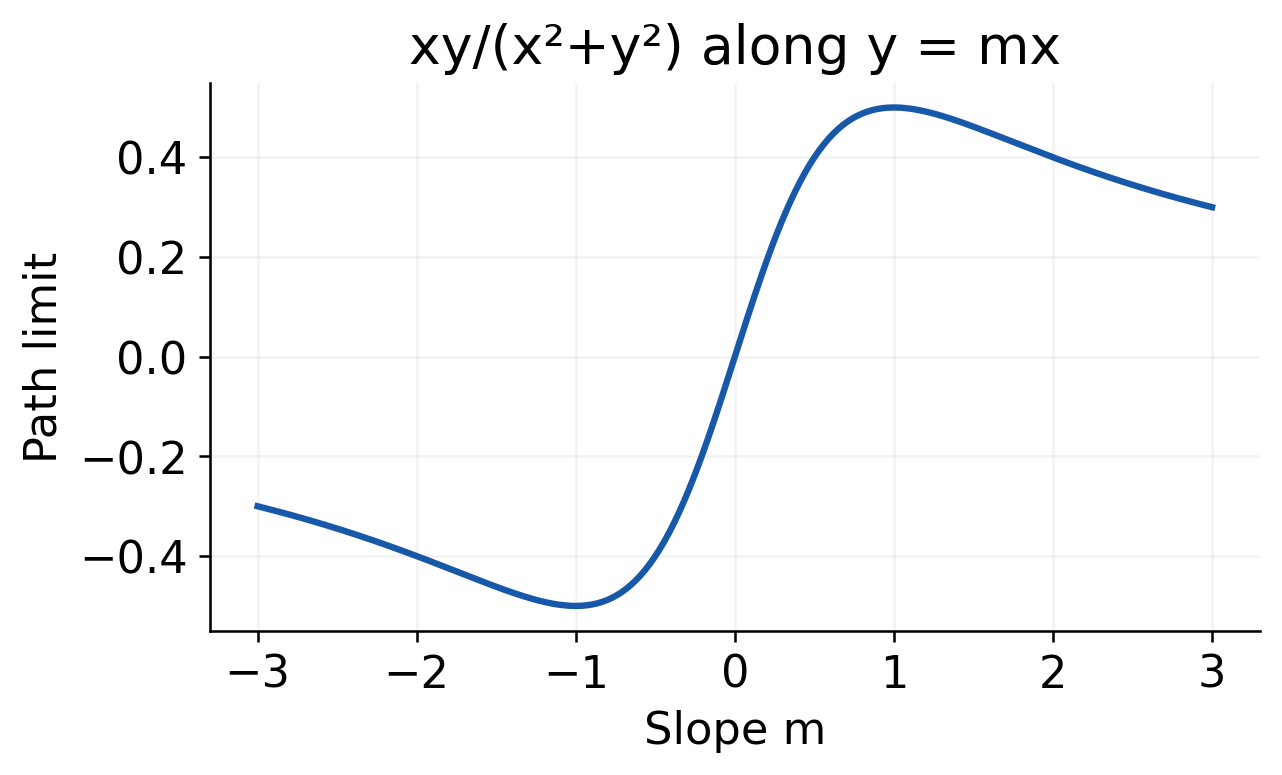
Along y=mx:
x(mx)/(x²+m²x²) = m/(1+m²)
The result depends on the slope m. This makes the failure especially clear: infinitely many line directions produce different limiting values.

What to Write in an Answer
Name each path, substitute it into the original expression, simplify for nonzero path parameter, and compare the resulting limits. State the conclusion explicitly.
Do not write only “depends on path” without showing the two calculations. Also check that the selected paths lie in the function’s domain near the target.
A Common Trap
Along x=0 and y=0, this particular function gives zero on both axes. The axes alone would therefore fail to detect the missing limit. The diagonal y=x supplies the needed contradiction.
Exam Shortcut: For rational expressions in x and y, the axes and y=mx are useful first probes. If their limits agree, continue investigating rather than declaring the full limit proved.
5. Straight Lines Can Be Misleading
Consider a function whose numerator and denominator contain different powers. The expression can hide a special curved approach even when every straight-line approach behaves well.
Worked Example 1.6: A Curved-Path Failure
Let:
f(x,y) = x²y/(x⁴+y²)
away from the origin.
For a nonzero fixed slope m and y=mx:
f(x,mx) = mx/(x²+m²) → 0
For m=0, the value is also zero. Along the vertical axis x=0, the value is zero for y≠0.
But along y=x²:
f(x,x²) = x⁴/(2x⁴) = 1/2
Thus the full limit does not exist, despite agreement along every straight line through the origin.
Choose Paths from the Denominator


The denominator contains x⁴ and y². Balancing those terms suggests y proportional to x², which makes both denominator terms have the same order.
This is a reasoning method, not a mechanical guarantee. A good path should expose a possible failure while staying in the domain.
Why Polar Substitution Alone May Fail
Writing x=r cos θ and y=r sin θ does not automatically prove a limit by taking r to zero with θ fixed. Fixed θ checks straight rays. A problematic θ can vary with r.
A valid polar proof needs a bound that is independent of θ, or another uniform argument controlling all directions.
A Practical Decision Tree
If two paths disagree, stop: the full limit fails. If selected paths agree, try a bound or a path adapted to the powers. Do not keep checking random lines indefinitely as a substitute for a proof.
Core Warning: “The answer is zero for every line y=mx” is not sufficient for the full two-variable limit to be zero.
A Family of Curved Approaches
The same failure can be seen along y=kx² with fixed k:
f(x,kx²) = k/(1+k²)
The resulting value varies with k, just as a line-slope family exposed the earlier example. Here the special scaling is quadratic rather than linear. Balancing the denominator terms suggests the appropriate family instead of leaving path selection to guesswork.
6. Proving a Limit with a Bound
A squeeze argument controls all nearby points at once. Let r=√(x²+y²). Useful inequalities include:
- |x|≤r
- |y|≤r
- 2|xy|≤x²+y²
Worked Example 1.7: A Uniform Squeeze
Find the limit of xy/√(x²+y²) at the origin, excluding the origin itself.
Using 2|xy|≤x²+y²:
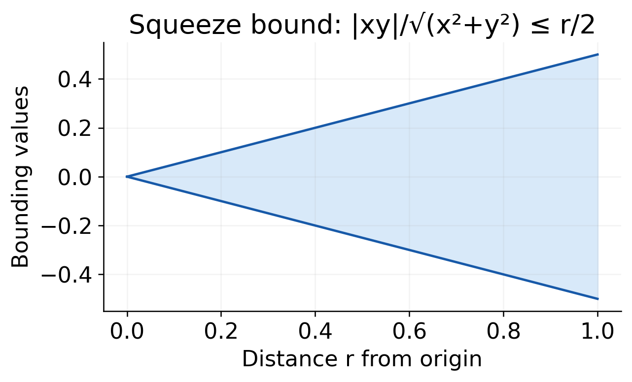
|xy/√(x²+y²)| ≤ r/2
Since r/2 approaches zero as r approaches zero, the function approaches 0 along every domain approach.

Worked Example 1.8: A Numerator of Higher Degree
For f=x³/(x²+y²), away from the origin:
|f| = |x|·x²/(x²+y²) ≤ |x| ≤ r
Thus the limit is zero. The estimate controls every approach and is shorter than checking many individual paths. The positive remaining length factor is what forces the value to vanish.
Worked Example 1.9: Polar Form with a Uniform Bound
For f(x,y)=x²y/(x²+y²), use x=r cos θ and y=r sin θ.
f = r cos²θ sin θ
Because |cos²θ sin θ|≤1 for every θ:
|f| ≤ r → 0
Therefore the full limit is 0.
The estimate is independent of θ, so it also covers approaches whose direction changes while approaching the origin.
Turning the Bound into ε–δ Language
If |f|≤r, choosing δ=ε is sufficient. If |f|≤r/2, choosing δ=2ε is sufficient. The exact numerical choice is not unique; it only needs to make the required implication true.
Check the Exponent of r
A positive remaining power of r multiplied by a uniformly bounded angular factor tends to zero. If the angular factor becomes unbounded or a denominator can approach zero, more analysis is needed.
Proof Habit: After a polar substitution, explicitly bound the angular expression. “Let r→0” without that step can hide an unjustified assumption about the approach direction.
7. Algebraic Limit Methods
Factoring, cancellation and rationalisation can convert an indeterminate expression into one controlled by standard limit laws. The original domain must still be respected.
Worked Example 1.10: Rationalise First
Evaluate the limit at the origin of:
[√(1+x²+y²)−1]/(x²+y²)
Multiply numerator and denominator by the conjugate. For (x,y)≠(0,0), the expression becomes:
1/[√(1+x²+y²)+1]
The new expression approaches 1/2 by continuity. The original quotient is undefined at the origin, but its limit exists.
Why Cancellation Is Legitimate
The equality is used only at nearby points where the cancelled factor is nonzero. A limit does not require the original and simplified formulas to agree at the excluded target point.
Worked Example 1.11: A Removable Quotient
For f(x,y)=(x²−y²)/(x−y), consider the limit at (1,1) through its domain x≠y.
Factor the numerator:
[(x−y)(x+y)]/(x−y) = x+y
The domain limit is therefore 2.
The original function is not defined on x=y. The simplified expression x+y defines a continuous extension, but this is an additional definition rather than an automatic change to the original function.
Domain-Sensitive Approaches
A path entirely contained in an excluded line is not an allowed path for the original function. In this example, using y=x to test the original quotient would be invalid because every point on that path is outside its domain.
Limit Laws Checklist
Check whether substitution is valid, whether denominator limits are nonzero, and whether a cancellation or conjugate gives an equivalent expression on nearby domain points. Use a path contradiction or a uniform bound when algebra alone does not resolve the issue.
Distinguish the Conclusions: “Undefined at the point,” “limit does not exist,” and “not continuous at the point” are different statements. An undefined function value does not by itself destroy a limit.
8. Continuity at a Point
A function is continuous at (a,b) when it is defined there, its domain limit there exists, and that limit equals the assigned value.
lim[(x,y)→(a,b)] f(x,y) = f(a,b)
At boundary points, the approach is restricted to the function’s domain. Ordinary polynomial functions are continuous everywhere; quotients of continuous functions are continuous where their denominators are nonzero.

Three Separate Checks
First check whether the point value exists. Next find or justify the limit. Finally compare the two. This order prevents an undefined expression from being mistaken for a missing limit automatically.
Worked Example 1.12: Choose the Point Value
Define f(x,y)=x²y/(x²+y²) away from the origin and set f(0,0)=c. Find c for continuity.
The uniform bound established earlier gives:
|x²y/(x²+y²)| ≤ √(x²+y²)
The surrounding limit is zero. Therefore continuity requires and is obtained by c=0.
Worked Example 1.13: No Point Value Can Help
Instead use f(x,y)=xy/(x²+y²) away from the origin and assign any number c at the origin.
Along y=0 the limit is 0; along y=x it is 1/2. Since the surrounding limit does not exist, no value of c makes the function continuous at the origin.
A Parameter Is Not a Proof
When a problem asks for a constant ensuring continuity, first establish that the limit exists independently of the point assignment. Simply substituting the target into an undefined quotient does not determine the parameter.
Continuity Summary: Existing limit plus matching point value gives continuity. A mismatched value is repairable; a path-dependent surrounding limit is not repairable by changing one point.
9. First Partial Derivatives
To differentiate f with respect to x, keep y fixed. To differentiate with respect to y, keep x fixed. Each operation is an ordinary one-variable derivative with the other input treated as a parameter.
fₓ(a,b) = lim[h→0] [f(a+h,b)−f(a,b)]/h
fᵧ(a,b) = lim[k→0] [f(a,b+k)−f(a,b)]/k
The limits must be interpreted where the relevant nearby inputs belong to the domain. A partial derivative at an interior point is a two-sided coordinate derivative.
Worked Example 1.14: Polynomial Partials
Let f=x²y+3xy². Holding y fixed gives:
fₓ = 2xy + 3y²
Holding x fixed gives:
fᵧ = x² + 6xy
At (1,2), fₓ=16 and fᵧ=13. The derivative values are not the function value, which is f(1,2)=14.
Why “Hold Fixed” Matters
The term 3xy² is linear in x when y is fixed, so its x derivative is 3y². It is quadratic in y when x is fixed, so its y derivative is 6xy.


First-Principles Check
For the x derivative of x²y at (a,b):
[(a+h)²b−a²b]/h = 2ab+bh
Letting h approach zero gives 2ab, matching the differentiation rule.
Units of a Partial
If f is measured in seconds and x in gigabytes, fₓ has units seconds per gigabyte with y fixed. A derivative can be interpreted only after identifying the output and input units.
Common Mistakes
Do not differentiate both x and y when a partial derivative is requested. Do not substitute a point too early if doing so would turn the function into a constant and erase the variable dependence.
Reliable Method: Differentiate symbolically while holding the correct inputs fixed, simplify, and only then evaluate at the requested point.

10. Partials of Composite Expressions
Product, quotient and chain rules still apply inside a partial derivative. The only change is which independent variables are treated as constants.
Worked Example 1.15: Exponential–Trigonometric Product
Let:
f(x,y) = e^(xy) sin x
When differentiating in x, both e^(xy) and sin x change:
fₓ = e^(xy)(y sin x + cos x)
When differentiating in y, sin x is constant:
fᵧ = xe^(xy) sin x
A missing factor y in the first expression or x in the second usually means the inner derivative of xy was omitted.
Check at a Simple Point
At (0,2), fₓ=1 and fᵧ=0. This agrees with the local x dependence of sin x and the fact that f(0,y) is identically zero.
Worked Example 1.16: Logarithmic Partials
For f=ln(x²+y²), the domain excludes the origin.
fₓ = 2x/(x²+y²)
fᵧ = 2y/(x²+y²)
At (1,1), both partial derivatives equal 1. The formulas do not define partial derivatives at the origin because the original logarithm is not defined there.
Worked Example 1.17: A Ratio Inside Arctangent
For f=arctan(y/x) on a chosen smooth branch with x>0:
fₓ = −y/(x²+y²)
fᵧ = x/(x²+y²)
Use the inner quotient derivatives before simplifying. The derivative formulas are local and do not make the angle a globally single-valued coordinate everywhere in the plane.
Formula Versus Domain
A simplified derivative can appear well-defined at a point where the original function is not. That does not create a derivative of the original function at the excluded point.
Chain-Rule Habit: For ln u, write uₓ/u. For eᵘ, write eᵘuₓ. For sin u, write cos u times uₓ. State which variables u depends on before choosing the inner derivative.
Worked Example 1.18: Quotient Partials
For f=(x+y)/(x−y), on x≠y, apply the quotient rule with the other coordinate fixed:
fₓ = −2y/(x−y)²
fᵧ = 2x/(x−y)²
The denominator is squared in both results, but the signs and numerators differ. Substituting x=y into the derivative formulas is invalid because the original function excludes that line.
11. Higher and Mixed Partials
A second partial derivative differentiates a first partial again. In these notes, fₓᵧ means differentiate fₓ with respect to y; fᵧₓ means differentiate fᵧ with respect to x.
fₓᵧ = ∂/∂y(∂f/∂x)
Worked Example 1.19: Compute All Second Partials
Let:
f = x³y² + sin(xy)
First:
fₓ = 3x²y² + y cos(xy)
fᵧ = 2x³y + x cos(xy)
Differentiating again:
fₓₓ = 6xy² − y² sin(xy)
fᵧᵧ = 2x³ − x² sin(xy)
The mixed derivative requires both a product derivative and an inner derivative of cos(xy):
fₓᵧ = 6x²y + cos(xy) − xy sin(xy)
Starting with fᵧ gives the same expression for fᵧₓ. This equality is expected because the function is smooth everywhere.
Worked Example 1.20: A Smooth Consistency Check
For f=e^(x+y), every first partial equals f. Differentiating again gives:
fₓₓ = fₓᵧ = fᵧₓ = fᵧᵧ = e^(x+y)
Hence fₓₓ+fᵧᵧ=2f. This is a useful quick check on the order notation: each operation differentiates the entire preceding function, while continuity makes the two mixed orders agree.
Organise the Work
Record fₓ and fᵧ on separate lines. Then compute fₓₓ, fₓᵧ, fᵧₓ and fᵧᵧ from the correct first derivative. A small derivative tree can prevent an order mix-up.
Values at a Point
For the function in Example 1.19, at (0,0), fₓₓ=0, fᵧᵧ=0 and both mixed partials equal 1. A mixed partial can therefore be nonzero even when the pure second partials at that point are zero.
Interpretation
A mixed partial describes how one coordinate slope changes when another coordinate changes. It is not a product of first partial derivatives.
For example, fₓᵧ is generally different from fₓfᵧ. The derivative notation represents an operation, not multiplication of subscripts.
Order Convention: Follow the explicitly stated meaning of fₓᵧ rather than guessing from a denominator layout. When second partials are continuous in a neighbourhood, the two mixed orders agree.
12. When Mixed Partials Agree
A standard sufficient condition for fₓᵧ=fᵧₓ near a point is continuity of the relevant second partial derivatives in a neighbourhood of that point. Smooth polynomial, exponential and trigonometric combinations satisfy the usual conditions on their domains.
Equality is not guaranteed merely because both mixed partials happen to exist at one point.
Worked Example 1.21: An Exceptional Origin
For nonzero (x,y), define:
f(x,y) = xy(x²−y²)/(x²+y²)
and set f(0,0)=0.
From the derivative definitions along the axes:
fₓ(0,y) = −y
fᵧ(x,0) = x
Both identities include their limiting values at the origin. Differentiating these axis functions gives:
fₓᵧ(0,0) = −1
fᵧₓ(0,0) = 1
The mixed partials exist but are unequal. The smoothness condition needed to interchange them at the origin is not satisfied.
Why Definitions Are Necessary Here
Away from the origin, the rational formula can be differentiated normally. At the specially defined origin, substituting directly into expressions with zero denominators is invalid. The partial definitions determine the required axis values.
The Function Itself Is Well Behaved in One Sense
Because |x²−y²|≤x²+y² and |xy|≤r²/2, the function satisfies |f|≤r²/2 near the origin. Hence it is continuous and even differentiable there with zero first-order linear part.
This does not force its mixed second derivatives to agree. First-order differentiability and continuous second derivatives are different levels of regularity.
Exam Response
State the sufficient theorem for ordinary smooth functions. If the question supplies a piecewise exceptional point, use definitions there and check the assumptions before interchanging derivative order.
Logic Warning: A sufficient condition is not a claim that equality can occur only under that condition. Failure of continuity means the theorem cannot be invoked; calculate rather than assuming either equality or inequality.
13. Geometry of Partial Slopes
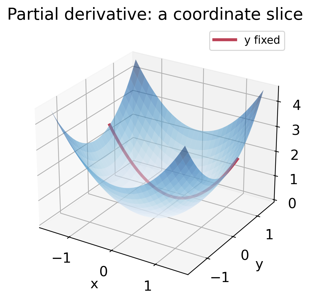
A partial derivative is the slope of a coordinate slice of the surface. For fₓ, move parallel to the x axis in the input plane while keeping y fixed.

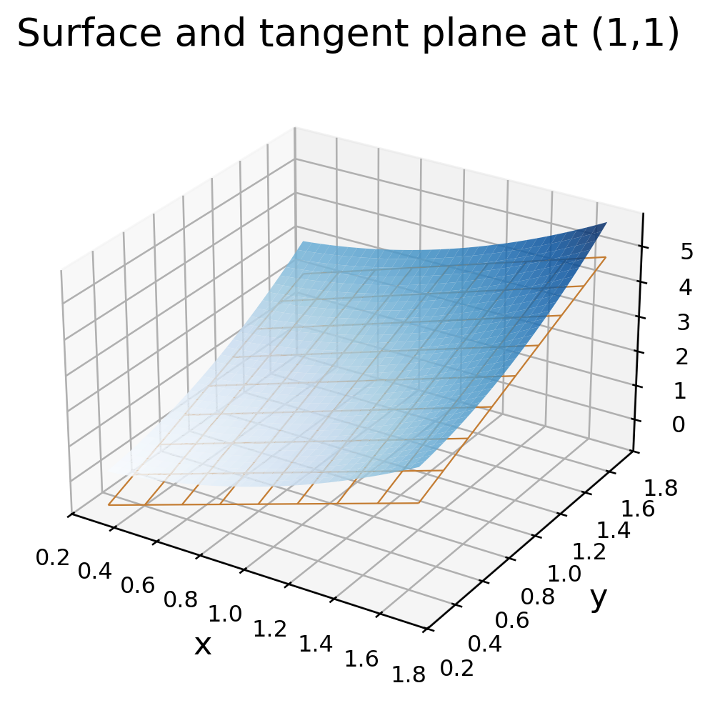
If f is differentiable at (a,b), the tangent plane is:
z = f(a,b)+fₓ(a,b)(x−a)+fᵧ(a,b)(y−b)
The two coordinate slopes combine into one local plane. Merely drawing two tangent lines does not prove that a valid plane approximates the surface in every direction.
Worked Example 1.22: Tangent Plane
For f=x²+y² at (1,1):
- f=2
- fₓ=2
- fᵧ=2
Therefore:
z = 2+2(x−1)+2(y−1)
Equivalently:
z = 2x+2y−2

Check the Contact Point
At x=y=1, the plane gives z=2. Its x and y coefficients are both 2, matching the corresponding partial slopes.
Local, Not Global
The plane is useful for small displacements near the contact point. It generally does not equal the surface far away. The mismatch is controlled by higher-order terms when the function is sufficiently smooth.
Geometric Meaning: Partial derivatives describe coordinate slopes. Differentiability allows those slopes to be assembled into a linear approximation valid for all small simultaneous displacements.
14. Differentiability: A Linear Approximation
Let h=x−a, k=y−b and r=√(h²+k²). A function is differentiable at (a,b) if a linear map gives its change with an error negligible compared with r.
f(a+h,b+k) = f(a,b)+Ah+Bk+R(h,k)
where:
R(h,k)/√(h²+k²) → 0
If this holds, A=fₓ(a,b) and B=fᵧ(a,b). The approximation must work for every small allowed displacement, not only the coordinate axes.
Differential Notation
The linear part is written:
df = fₓ dx + fᵧ dy
The actual finite change Δf need not equal df exactly. Differentiability states that their difference becomes small relative to the input displacement.
Worked Example 1.23: Product Increment
For f=xy at (a,b), the exact increment is:
Δf = bh+ak+hk
The candidate differential is bh+ak, leaving R=hk. Since 2|hk|≤h²+k²:
|R|/r ≤ r/2 → 0
This proves differentiability without relying solely on a theorem about continuous partials. It also identifies the exact term neglected by the differential.
Worked Example 1.24: Verify Differentiability
For f=x²+y² at an arbitrary point (a,b):
f(a+h,b+k)−f(a,b) = 2ah+2bk+h²+k²
The proposed linear part is 2ah+2bk. Its remainder is R=h²+k²=r². Thus:
|R|/r = r → 0
Therefore f is differentiable everywhere, with fₓ=2a and fᵧ=2b at the point.
Why This Is Stronger Than Continuity
Continuity requires Δf→0. Differentiability additionally identifies a linear first-order part and requires the remaining error to vanish relative to the displacement length.
A Practical Remainder Test
Compute the exact increment, subtract the candidate linear part, and divide by r. Bound the resulting expression uniformly or demonstrate a path where it fails to approach zero.
If partials exist, the candidate linear part is already determined. You cannot choose unrelated coefficients later to repair a failed differentiability test.
Key Implication: Differentiability implies continuity and existence of the first partials. The reverse implication from existing partials alone is false.
When Linearisation Is Exact
If f is affine, f=c+Ax+By with constants A and B, the remainder is identically zero. Its differential equals every finite increment, not just a nearby approximation.
Nonlinear functions generally have a remainder; differentiability says how that remainder behaves relative to the displacement as the displacement shrinks.
15. Existing Partials Are Not Enough
Return to:
f = xy/√(x²+y²)
away from the origin, with f(0,0)=0. The bound |f|≤r/2 proves continuity at the origin.
Along either coordinate axis, the function is zero. Therefore the first partial derivatives at the origin both exist and equal zero.
If f were differentiable there, its linear part would be zero. The required test would be:
f(h,k)/√(h²+k²) → 0
Worked Example 1.25: Test the Diagonal
Along h=k=t with t≠0:
f(t,t) = |t|/√2
The distance to the origin is √2|t|, giving:
f(t,t)/√(t²+t²) = 1/2
The ratio does not approach zero. Thus f is not differentiable at the origin, despite continuity and both first partials there.
Why the Coordinate Checks Missed It

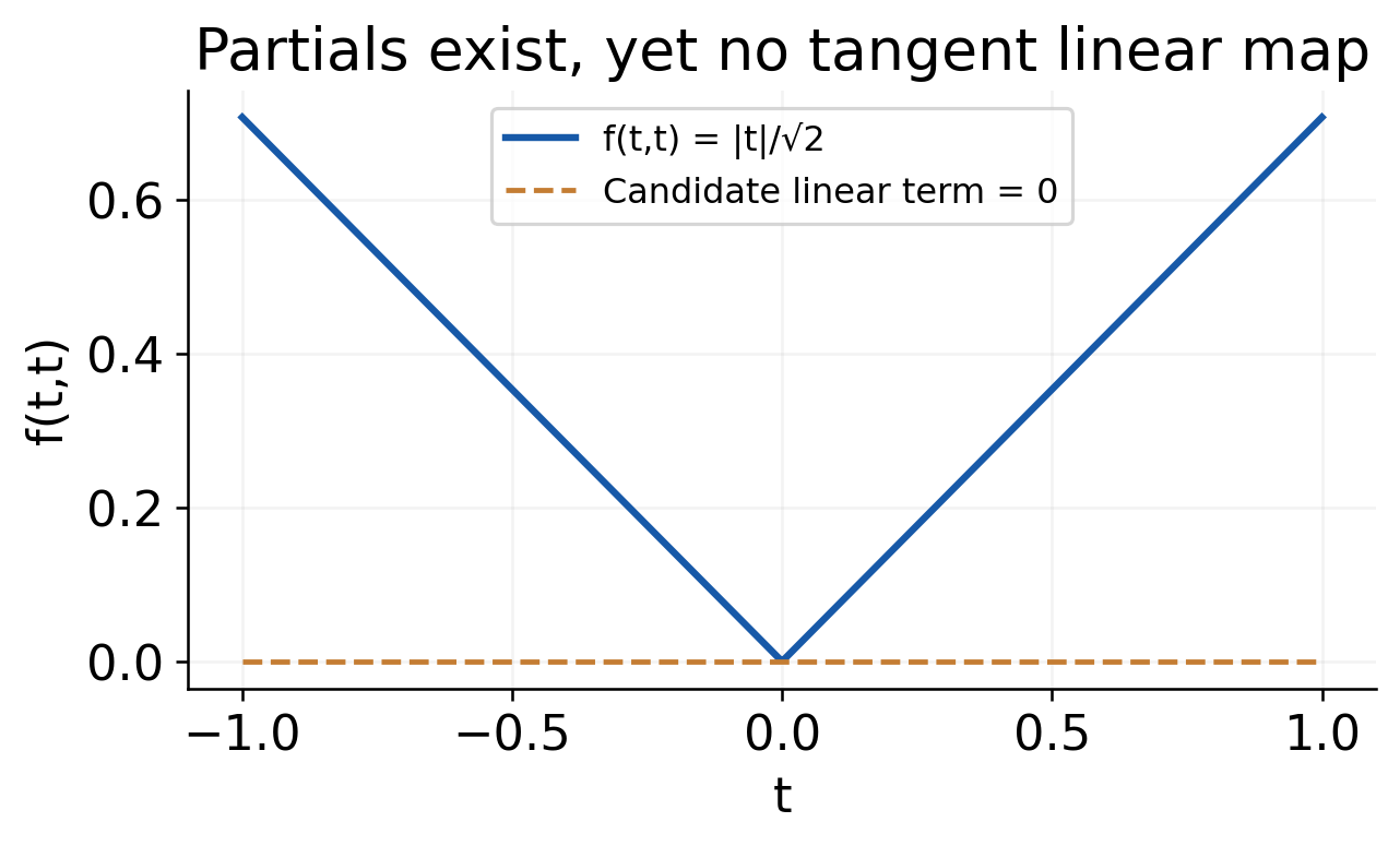
A partial derivative probes just one coordinate direction. The differentiability condition controls arbitrary simultaneous changes of both coordinates.
Three Conditions Compared
| Statement | What It Controls |
|---|---|
| Continuity | Output approaches the point value |
| First partials exist | Coordinate-direction rates exist |
| Differentiability | One linear map approximates all small changes |
The first two together still do not imply the third. This counterexample is useful because the failed differentiability ratio is a nonzero constant, making the contradiction explicit.
How to Present the Answer
Show the point value, establish continuity with a bound if needed, calculate partials by definition and then test the remainder ratio. Stopping after the partial derivatives would leave the main question unanswered.
Remember the Distinction: A surface can have well-defined coordinate slopes at a point without having one tangent plane that gives the correct first-order behaviour in every direction.
16. A Useful Sufficient Condition
If the first partial derivatives exist in an open neighbourhood of a point and are continuous there, the function is differentiable at the point. This C¹ condition is easy to check for many standard formulas.
It is sufficient, not necessary: some differentiable functions have first partials that are not continuous at the point. Use the theorem when it applies, and use a remainder argument when the theorem does not settle the problem.
Worked Example 1.26: Linearise a Square Root
Let f=√(x²+y²), near (3,4). Since the origin is not nearby, its partials are continuous in a suitable neighbourhood.
f(3,4)=5
fₓ = x/√(x²+y²)
fᵧ = y/√(x²+y²)
At (3,4), the slopes are 3/5 and 4/5. Hence:
f(3+h,4+k) ≈ 5+(3/5)h+(4/5)k
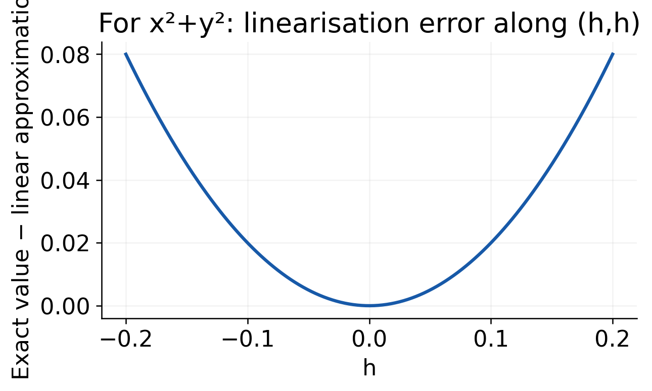
Evaluate the Approximation
For (x,y)=(3.02,3.99), h=0.02 and k=−0.01:
df = (3/5)(0.02)+(4/5)(−0.01) = 0.004
The linear estimate is 5.004. The exact value is √25.0405≈5.004048, close to the estimate for this small displacement.
Why It Is Close
The neglected higher-order contribution is small in a neighbourhood where the function is smooth. A small displacement is useful only relative to the local variation and domain; linearisation near a singular point needs special care.

Implication Map
C¹ near the point implies differentiability. Differentiability implies continuity and partial derivatives. Existing partials, even together with continuity, do not alone guarantee differentiability.
Calculation Habit: Choose a nearby easy base point, compute its value and partials, insert the small signed changes and state that the result is an approximation.


17. Composite Functions: One Parameter
Suppose z=f(x,y), while x=x(t) and y=y(t). A change in t reaches z through two dependence paths. If the required functions are differentiable, the chain rule adds those contributions.
dz/dt = fₓ(dx/dt)+fᵧ(dy/dt)

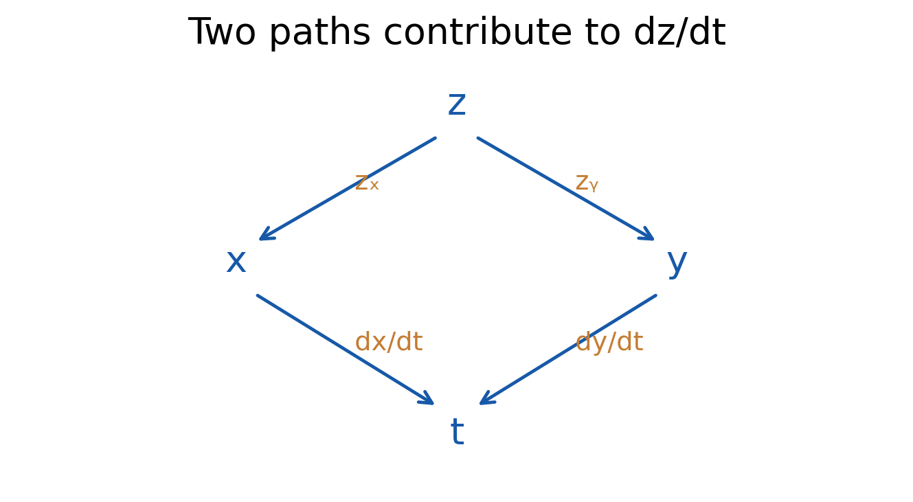
The derivative dz/dt is a total derivative along the specified input path. It is not generally the same as a partial derivative that holds another input fixed.
Before Calculating
Name the outer function, identify the inner functions and calculate each inner derivative separately. Evaluate all factors at compatible input values.
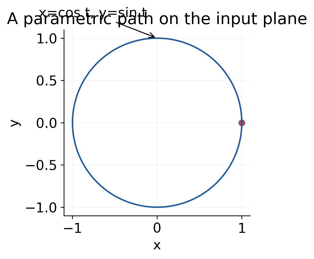
Worked Example 1.27: Change Along a Circle
For z=x²+y² with x=cos t and y=sin t:
dz/dt = 2 cos t(−sin t)+2 sin t cos t = 0
The output is constant because the input follows a level circle. Both branch contributions are nonzero in general, but they cancel. Ignoring either dependence path would incorrectly predict a changing output.
Worked Example 1.28: Two Changing Inputs
Let z=x²y, x=t² and y=eᵗ. Then fₓ=2xy and fᵧ=x², while x′=2t and y′=eᵗ.
dz/dt = 2xy(2t)+x²eᵗ
Substitute the inner functions:
dz/dt = eᵗ(4t³+t⁴)
At t=1, the derivative is 5e.
Independent Substitution Check
Directly, z(t)=t⁴eᵗ. The ordinary product rule gives the same expression. This is a useful check when direct substitution remains manageable.
Why Both Branches Matter
The factor x² changes because x changes, while the factor y changes independently. Ignoring y′ loses a real contribution even if the outer formula is simple.
Parametric Meaning
A curve t↦(x(t),y(t)) selects how the input moves. The same surface can give different total rates along different paths through one point because the input velocity differs.
Chain-Rule Rule: Multiply derivatives along each dependence path and add across paths. Keep the total derivative on the left and the appropriate partial derivatives of the outer function on the right.
18. Composite Functions: Two Parameters
Let z=f(x,y), with x=x(u,v) and y=y(u,v). When taking the u partial, hold v fixed; when taking the v partial, hold u fixed.
zᵤ = fₓxᵤ+fᵧyᵤ
zᵥ = fₓxᵥ+fᵧyᵥ
Each term is a product of an outer partial and an inner partial. The fully written derivative form makes the dependence unambiguous:
∂z/∂u = (∂f/∂x)(∂x/∂u)+(∂f/∂y)(∂y/∂u)
Use a separate dependence tree for each independent parameter, or annotate one tree with which parameter is held fixed.
Worked Example 1.29: Exponential Polar Inputs
Let z=ln(x²+y²), x=eᵘ cos v and y=eᵘ sin v. Since x²+y²=e^(2u), direct substitution gives z=2u.
For a chain-rule check:
- xᵤ=x
- yᵤ=y
- xᵥ=−y
- yᵥ=x
Therefore:
zᵤ = (2x²+2y²)/(x²+y²) = 2
zᵥ = (−2xy+2xy)/(x²+y²) = 0
The radius is always positive, so the logarithm’s origin singularity is avoided.
Worked Example 1.30: A Polynomial Transformation
Let z=x²+y², x=u+v and y=uv.
For the u derivative, xᵤ=1 and yᵤ=v:
zᵤ = 2(u+v)+2uv²
For the v derivative, xᵥ=1 and yᵥ=u:
zᵥ = 2(u+v)+2u²v
At (u,v)=(1,2), zᵤ=14 and zᵥ=10.
Direct Check
Substitution gives z=(u+v)²+u²v². Differentiating this expression with respect to u or v gives the same results.
Holding Fixed Changes with Coordinates
The statement “v fixed” does not mean “y fixed,” because y=uv can change when u changes even at fixed v. A new coordinate system changes what a coordinate partial derivative follows in the original input plane.
Notational Care
Write a product dot or full derivative fractions if adjacent subscripts could be confused. A chain-rule product is not a higher-order partial derivative.
Practical Check: After evaluating at (u,v), make sure x and y are evaluated at the transformed point. Do not mix outer derivatives at one location with inner derivatives at another.
Interpret the New Coordinates
For the exponential polar transformation:
| Change with Other New Input Fixed | Effect in the Original Plane |
|---|---|
| Increase u | Increase positive radius eᵘ |
| Increase v | Rotate at fixed radius |
The output depends on radius and is unchanged by rotation. Although the transformed expression is simple, the map is periodic in v. A simple composite formula does not establish a global inverse over all real angle values.
19. Implicit Partial Differentiation
If an equation F(x,y,z)=0 locally defines z as a differentiable function of x and y, the chain rule gives formulas for zₓ and zᵧ when F_z≠0.
zₓ = −Fₓ/F_z
zᵧ = −Fᵧ/F_z
The derivatives of F in these formulas treat x, y and z as independent arguments before the implicit relation is imposed.
Worked Example 1.31: A Sphere Branch
Let x²+y²+z²=9 on the upper branch near (1,2,2). Then Fₓ=2x, Fᵧ=2y and F_z=2z.
zₓ = −x/z
zᵧ = −y/z
At the specified point, zₓ=−1/2 and zᵧ=−1. The denominator is nonzero there, so the local formula is valid.
Worked Example 1.32: A Mixed Implicit Curve
For x²+xy+y²=7 near (1,2), implicit differentiation gives:
(2x+y)+(x+2y)(dy/dx) = 0
Therefore:
(dy/dx) at (1,2) = −4/5
The denominator x+2y equals 5 at the point, so the local y(x) derivative is valid. The point satisfies the original equation, which should always be checked before evaluating an implicit slope.
A Related One-Curve Example
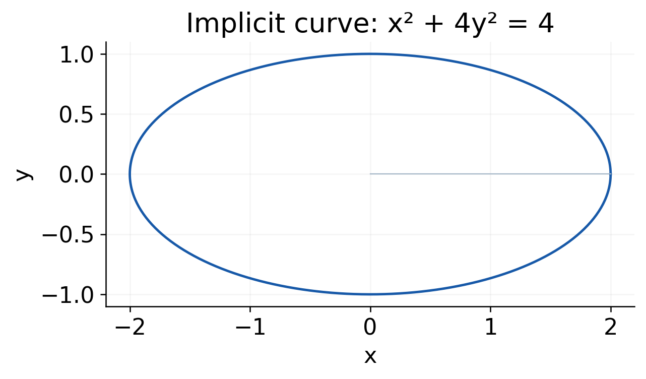
For x²+4y²=4 with y locally a function of x:
2x+8y(dy/dx) = 0
dy/dx = −x/(4y), y≠0

Why the Denominator Condition Matters
At y=0 on this ellipse, dividing by 4y is invalid. This does not mean the entire curve disappears. It means that the chosen representation y(x) fails the nonzero-derivative condition at that point.
Similarly, on the sphere’s equator, z cannot be described by the same smooth upper-branch graph over every nearby x–y point.
Sign Check
For x>0 and y>0 on the ellipse, increasing x forces y to decrease, so dy/dx is negative. Geometrical reasoning helps catch a missing minus sign.
Method: Differentiate the constraint, isolate the required derivative and state the nonzero denominator condition. A formula without that condition can be misused precisely where the graph representation breaks down.
20. Total Derivatives with Explicit Dependence
A quantity may depend on t directly as well as through x(t) and y(t). If z=f(x,y,t), the total derivative contains all three contributions.
dz/dt = fₓ(dx/dt)+fᵧ(dy/dt)+fₜ
The last term is the explicit t partial with x and y held fixed. Omitting it ignores a genuine dependence path.
Worked Example 1.33: Direct and Indirect Changes
Let z=x²y+ty, x=t² and y=1+t. The outer partials are:
fₓ=2xy, fᵧ=x²+t, fₜ=y
Using x′=2t and y′=1:
dz/dt = 4txy+x²+t+y
After substitution:
dz/dt = 5t⁴+4t³+2t+1
At t=1, the total derivative is 12.

Check by Direct Substitution
The original expression becomes:
z(t) = t⁴(1+t)+t(1+t)
Ordinary differentiation gives 4t³+5t⁴+1+2t, agreeing with the chain rule.
Moving-Input Interpretation
Suppose f describes a position-dependent measurement with an explicitly time-changing background. A moving observer experiences both changes due to position and changes that occur even at a fixed position.
The same logic applies to a performance model whose workload and capacity change while an explicit time-dependent overhead also changes. These are model dependencies, not an assumption that every physical system has the same formula.
Differentials as Bookkeeping
For independent variables x,y,t:
df = fₓ dx+fᵧ dy+fₜ dt
Substituting dx=x′dt and dy=y′dt recovers the total derivative along the path.
Common Confusion
The symbol fₜ is not the same as dz/dt after x and y have been made functions of t. The former holds them fixed; the latter includes their motion.
Dependence Check: List every direct and indirect route from the changing parameter to the output before writing the derivative. Missing a route is more common than a difficult algebraic error.
21. Change of Variables and Operators
A coordinate change can simplify differentiation. Let u=x+y and v=x−y, and write f(x,y)=F(u,v).


Since uₓ=vₓ=1 and uᵧ=1, vᵧ=−1, the chain rule yields:
∂/∂x = ∂/∂u+∂/∂v
∂/∂y = ∂/∂u−∂/∂v
These identities act on suitable differentiable composite functions. They are not equations between ordinary numerical fractions.
Worked Example 1.34: Use Transformed Derivatives
Let F(u,v)=u²v. Its partials are F_u=2uv and F_v=u². Hence:
fₓ = 2uv+u²
fᵧ = 2uv−u²
At (x,y)=(1,2), the transformed point is (u,v)=(3,−1), giving fₓ=3 and fᵧ=−15.
Second-Order Identity
If the function is C² and the transformation coefficients are constant:
fₓₓ+fᵧᵧ = 2(F_uu+F_vv)
The mixed terms cancel when the two operator squares are added. With a nonlinear transformation, the coefficients also vary and must themselves be differentiated.
Why This Is Useful
Changing variables can expose symmetry, simplify a differential expression or organise a composite derivative. The transformation does not remove the need to state which coordinates are independent.
Inverse Transformation
The same linear relations give x=(u+v)/2 and y=(u−v)/2. Substituting them provides an independent way to differentiate the re-expressed function.
Operator Warning: Do not square a variable-coefficient differential operator as if its coefficients were constants. Apply the operator to the entire next expression, including coefficient functions.
22. Homogeneous Functions and Euler
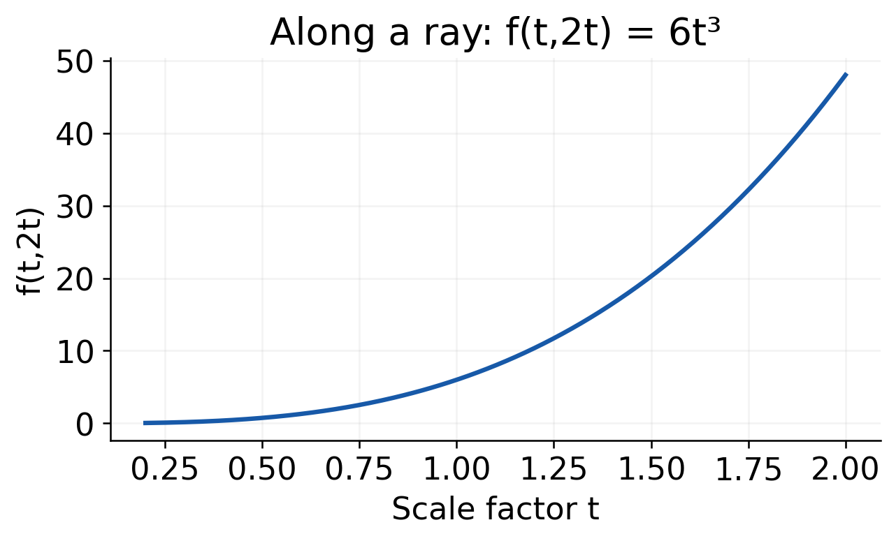
A function is homogeneous of degree n on a suitable scaling domain if:
f(tx,ty) = tⁿf(x,y), t>0
Positive scaling avoids unnecessary ambiguity for fractional powers and restricted real domains. The points used must remain in the domain.
Examples
- x²+xy+y² has degree 2.
- x²y+y³ has degree 3.
- (x³+y³)/(x+y) has degree 2 where its denominator is nonzero.
A sum such as x²+y³ is not homogeneous of one degree because its terms scale differently. Expressions involving a ratio y/x can have degree zero on an appropriate domain.
Euler’s Theorem
If f is differentiable and homogeneous of degree n:
xfₓ+yfᵧ = nf
The identity connects coordinate derivatives with a radial scaling change of the inputs.
Worked Example 1.35: Reject a False Degree
For f=x²+y³, scaling produces t²x²+t³y³. No single degree works throughout an open scaling domain. Direct differentiation confirms:
xfₓ+yfᵧ = 2x²+3y³
It cannot equal nf for one constant n at all inputs: the coefficients would require n=2 and n=3 simultaneously. Homogeneity belongs to the whole function, not whichever term is inspected first.
Leonhard Euler


Short Derivation
Hold x and y fixed and differentiate f(tx,ty)=tⁿf(x,y) with respect to t. The chain rule gives:
xfₓ(tx,ty)+yfᵧ(tx,ty) = nt^(n−1)f(x,y)
Setting t=1 gives Euler’s identity. This proof also explains why differentiability and a valid scaling domain are needed.
Radial Interpretation
The weighted derivative xfₓ+yfᵧ describes the first-order response when both coordinates are scaled together. It is not the rate obtained by changing only x or only y.
Homogeneity Test: Replace every x and y by tx and ty, factor the resulting power of t and check that the remaining expression is exactly the original function. Guessing from one term can miss a nonhomogeneous sum.
23. Verifying Euler’s Identity
Homogeneity can simplify a derivative combination, but a verification question usually requires both identifying the degree and computing the needed partials.
Worked Example 1.36: A Homogeneous Cubic
Let:
u = x³+3x²y+2y³
Every monomial has total degree 3, so u is homogeneous of degree 3.
uₓ = 3x²+6xy
uᵧ = 3x²+6y²
Therefore:
xuₓ+yuᵧ = 3x³+9x²y+6y³ = 3u
This verifies Euler’s theorem rather than merely quoting it.

Numerical Verification at (1,2)
For the cubic u=x³+3x²y+2y³:
- u=23
- uₓ=15
- uᵧ=27
Hence:
xuₓ+yuᵧ = 15+2(27) = 69 = 3(23)
This checks the derivative identity at one point after the symbolic verification. A point check alone would not prove the identity throughout the domain.
Worked Example 1.37: A Fractional Power
Let u=(x²+y²)^(3/2). For t>0, u(tx,ty)=t³u(x,y), so the degree is 3.
Writing r=√(x²+y²), away from the origin:
uₓ=3xr, uᵧ=3yr
Hence:
xuₓ+yuᵧ = 3r(x²+y²) = 3r³ = 3u
At the origin the same identity is consistent with zero first derivatives, which can be checked from the definition.
Why Positive Scaling Was Stated
For a square root or fractional power, replacing t by a negative number can introduce |t| rather than t. The standard local positive-scaling definition avoids claiming an invalid algebraic identity.
Ratio Example
For u=(x³+y³)/(x+y), count numerator degree 3 minus denominator degree 1 to obtain degree 2, provided the denominator is nonzero. Domain restrictions survive even if algebra later simplifies the expression.
Efficient Use: If only xuₓ+yuᵧ is requested and homogeneity is established, Euler gives the answer directly. If a verification is requested, show the derivatives and substitution as well.
24. Higher-Order Euler Identities
Suppose f is C² and homogeneous of degree n. Differentiate xfₓ+yfᵧ=nf in x and y:
xfₓₓ+yfₓᵧ = (n−1)fₓ
xfₓᵧ+yfᵧᵧ = (n−1)fᵧ
Multiplying the first relation by x, the second by y, and adding gives:
x²fₓₓ+2xyfₓᵧ+y²fᵧᵧ = n(n−1)f
The equality of the mixed derivatives is used under the stated smoothness assumption. The expression is a weighted combination of second partials, not simply the square of Euler’s first left-hand side.
What Changes for Three Variables?
The first identity becomes xfₓ+yfᵧ+zf_z=nf. Higher-order versions include every corresponding mixed term with its correct multiplicity.
Worked Example 1.38: Degree Zero
For f=y/x on x≠0, the degree is zero. Its relevant second partials are:
fₓₓ=2y/x³, fₓᵧ=−1/x², fᵧᵧ=0
The weighted combination is 2y/x−2y/x=0, matching n(n−1)f.
A degree-zero function need not be constant as the input direction changes; it is constant only under the allowed common scaling.
Worked Example 1.39: Quadratic Check
For f=x²+xy+y², n=2:
fₓₓ=2, fₓᵧ=1, fᵧᵧ=2
Then:
x²fₓₓ+2xyfₓᵧ+y²fᵧᵧ = 2x²+2xy+2y² = 2f
This agrees with n(n−1)f=2f.
Why n² Is a Common Wrong Answer
Let D=x∂/∂x+y∂/∂y. Applying D twice gives D²f=n²f. But expanding D² also differentiates the coefficient functions x and y.
The weighted second-derivative combination equals D²f−Df, so its value is n²f−nf=n(n−1)f.
Third-Order Extension
With enough smoothness, the analogous cubic weighted combination has coefficient n(n−1)(n−2). This is an extension of the same scaling logic; write all mixed terms carefully rather than copying only the pure derivatives.
Shortcut Check: For degree 1, the weighted second-order combination is zero. For degree 2, it is 2f. These simple cases help detect an incorrect coefficient in a memorised formula.
Worked Example 1.40: Third-Order Cubic Check
For f=x³+y³, the pure third partials are both 6 and the mixed third partials vanish. The cubic weighted combination is:
6x³+6y³ = 3·2·1 f
This verifies the coefficient n(n−1)(n−2) for n=3. Keep the smoothness requirement and all mixed terms in the general identity even when this simple example makes them zero.
25. Functions Built from Homogeneous Inputs
A logarithm or inverse trigonometric function of a homogeneous expression need not itself be homogeneous of the same degree. Apply the ordinary chain rule to the inner homogeneous function.
If u=φ(v) and v is homogeneous of degree n:
xuₓ+yuᵧ = φ′(v)(xvₓ+yvᵧ)
Therefore:
xuₓ+yuᵧ = nvφ′(v)
This form avoids the incorrect assumption that the answer must always be nu.
Worked Example 1.41: Logarithm of a Quadratic
For u=ln(x²+y²), let v=x²+y². Its degree is 2, and φ′(v)=1/v.
xuₓ+yuᵧ = 2v(1/v) = 2
This holds on the domain excluding the origin. The result is 2, not 2u.
Worked Example 1.42: An Inverse-Sine Transformation
Let u=arcsin v, with v=(x³+y³)/(x+y). The inner function has degree 2. On a smooth real domain with x+y≠0 and |v|<1:
xuₓ+yuᵧ = 2v/√(1−v²) = 2 tan u
The restriction |v|<1 keeps the derivative denominator nonzero. It is not enough that the inverse sine itself is defined at an endpoint.
Scaling Inside the Logarithm


Worked Example 1.43: Arctangent of a Quadratic
Let u=arctan(x²+y²), with v=x²+y² of degree 2.
xuₓ+yuᵧ = 2v/(1+v²)
Since tan u=v, this can also be written:
xuₓ+yuᵧ = sin(2u)
The trigonometric rewriting is optional; the rational expression already gives the derivative combination correctly.
Degree-Zero Comparison
For u=arctan(y/x) on a suitable smooth branch, the ratio y/x has degree zero. The whole function is unchanged by positive scaling, so its Euler weighted derivative is zero.
Transformed-Function Method: Identify the inner homogeneous expression, find its degree, differentiate the outer function and then simplify. This is safer than assigning a degree to a logarithm by inspection.
26. Taylor Expansion in Two Variables
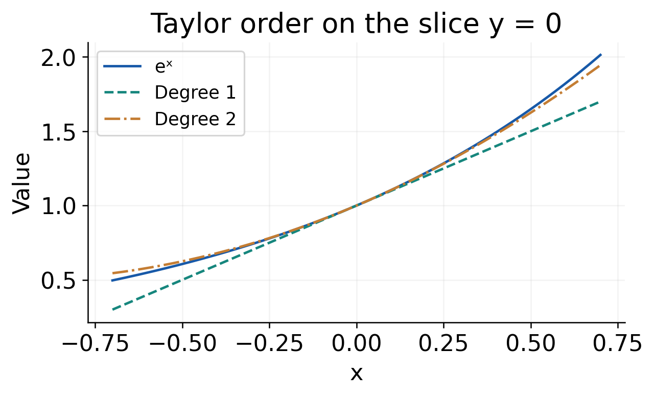
A Taylor expansion approximates a smooth function near a base point (a,b). Write h=x−a and k=y−b. All derivative coefficients are evaluated at the base point.
The second-degree polynomial is:
T₂ = f₀+h(fₓ)₀+k(fᵧ)₀+½[h²(fₓₓ)₀+2hk(fₓᵧ)₀+k²(fᵧᵧ)₀]
Here f₀=f(a,b). The mixed term has coefficient 2 inside the bracket; after multiplication by 1/2, its coefficient is hk(fₓᵧ)₀.
With continuous second derivatives, the remainder after T₂ is smaller than r² in the Peano sense. With appropriately bounded third derivatives nearby, a third-order remainder bound can be obtained.
First-Degree Approximation
T₁ = f₀+h(fₓ)₀+k(fᵧ)₀
This is the tangent linear approximation. T₂ adds local curvature, including interaction between simultaneous x and y changes.
Brook Taylor


A Dependable Construction Method
- Choose the base point and calculate h and k.
- Compute f, first partials and second partials at that point.
- Substitute those fixed coefficient values into T₂.
- Simplify the polynomial in h and k.
- If a numerical approximation is requested, insert the signed changes last.
- State the degree and the neglected higher-order terms or assumptions.
Common Coefficient Error
Forgetting the factor 2 in the mixed term gives half its correct contribution. Treating h and k as the original x and y without shifting also gives a wrong expansion away from the origin.
Base-Point Rule: The Taylor polynomial has variable h and k but fixed derivative coefficients. Leaving coefficients as functions of the moving point does not produce the intended expansion about (a,b).
Why the Mixed Coefficient Is Two
Treat h and k as fixed increments and introduce the operator D=h∂/∂x+k∂/∂y. Under the smoothness conditions allowing mixed derivatives to agree:
D²f = h²fₓₓ+2hkfₓᵧ+k²fᵧᵧ
Taylor’s second-degree term is D²f/2 evaluated at the base point. This operator view explains the coefficient rather than asking you to memorise it without a reason.
27. Taylor Expansion About a Nonzero Point
Worked Example 1.44: A Cubic Around (1,1)
Let f=x²y+xy². At (1,1):
f₀=2, (fₓ)₀=3, (fᵧ)₀=3
(fₓₓ)₀=2, (fₓᵧ)₀=4, (fᵧᵧ)₀=2
With h=x−1 and k=y−1:
T₂ = 2+3h+3k+h²+4hk+k²
The exact substitution into the cubic gives:
f(1+h,1+k) = T₂+h²k+hk²
Thus the omitted part is exactly cubic in the increments. No infinite-series convergence issue is needed for this polynomial identity.
Why Shifting Matters
The coefficients 3 and 3 are the slopes at (1,1), not at the origin. The same function expanded about a different point has different lower-degree coefficients.
Worked Example 1.45: An Exact Quadratic Expansion
For f=x²+xy+y² at (1,2):
- Value = 7
- First partials = 4 and 5
- Second partials = 2,1,2
With h=x−1 and k=y−2:
f(1+h,2+k) = 7+4h+5k+h²+hk+k²
Because the original function is quadratic, there are no terms of higher degree. The second-degree Taylor polynomial is exact here, whereas the first-degree one still omits the quadratic change.
Worked Example 1.46: Data-Processing Approximation
For two sequential stages with no overlap, per-item times 1/a and 1/b give the simplified processing rate:
p = ab/(a+b)
with positive stage rates a and b.
At (a,b)=(4,6), p=2.4 and the partial sensitivities are:
p_a = b²/(a+b)² = 0.36
p_b = a²/(a+b)² = 0.16
For changes 0.1 and 0.2:
p_new ≈ 2.4+0.36(0.1)+0.16(0.2) = 2.468
The exact model value is 25.42/10.3≈2.467961. The no-overlap assumption is essential; a pipelined system would require a different performance model.
Evaluate and Check the Cubic Approximation
For the function in Example 1.44, at (x,y)=(1.10,1.05), h=0.10 and k=0.05:
T₂ = 2+0.30+0.15+0.01+0.02+0.0025 = 2.4825
The exact cubic remainder is:
h²k+hk² = 0.0005+0.00025 = 0.00075
So the exact value is 2.48325.
Compare Taylor Degrees
The first-degree estimate would be T₁=2.45. The quadratic terms improve the estimate for this example. Higher degree often helps locally, but the actual error also depends on the function, point and displacement.
A Useful Independent Check
Expand the original polynomial directly after replacing x by 1+h and y by 1+k. Group terms by total degree: constants, linear, quadratic and cubic. These groups must match the Taylor construction.
Total Degree, Not Separate Degree
The term h²k is degree 3, not degree 2. A second-degree two-variable expansion retains terms whose combined exponent is at most 2.
Sorting Trick: Keep 1, h, k, h², hk and k² for degree 2. Terms such as h²k, hk² and h³ belong to the next total degree.
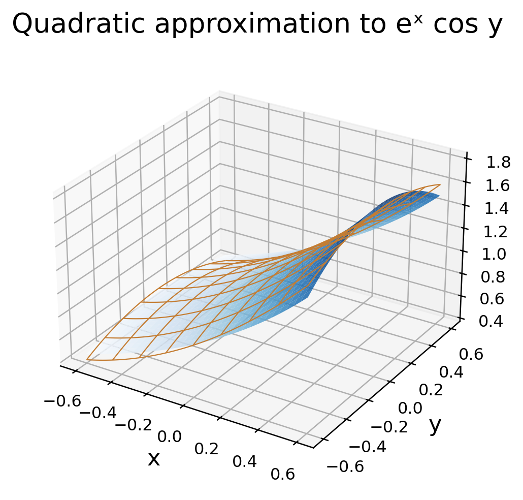
28. Taylor Expansion of a Transcendental Function
Worked Example 1.47: Expand eˣ cos y
At the origin:
- f=1
- fₓ=1
- fᵧ=0
- fₓₓ=1
- fₓᵧ=0
- fᵧᵧ=−1
Therefore:
T₂(x,y) = 1+x+(x²−y²)/2
The third-degree terms are:
(x³−3xy²)/6
Hence:
T₃ = T₂+x³/6−xy²/2
The missing y and xy terms are zero because their corresponding coefficients vanish at the base point.

Numerical Comparison
At x=0.10 and y=0.20:
T₂ = 1+0.10+(0.01−0.04)/2 = 1.085
The cubic correction is −0.00183333, giving:
T₃ ≈ 1.08316667
The exact value is:
exp(0.1) cos(0.2) ≈ 1.08314108

Alternative Derivation
Multiply the one-variable series for eˣ and cos y, then retain only terms of the requested total degree. This gives an independent check on the partial-derivative method.
Local Validity
A Taylor polynomial is centred at one point. Its use at a remote point requires an error or convergence argument, not merely a higher polynomial degree.
Accuracy Check: Compare the numerical estimate with an exact evaluation when available, but keep that check separate from the derivation. A matching decimal alone does not explain the expansion coefficients.
29. Expansion and Local Shape
At a stationary point, first partials vanish. The second-degree Taylor contribution then describes the leading local shape if its quadratic form is definite.
Q(h,k) = ½(Ah²+2Bhk+Ck²)
Here A=fₓₓ, B=fₓᵧ and C=fᵧᵧ at the stationary point. The mixed coefficient can rotate or tilt the level curves relative to the coordinate axes.

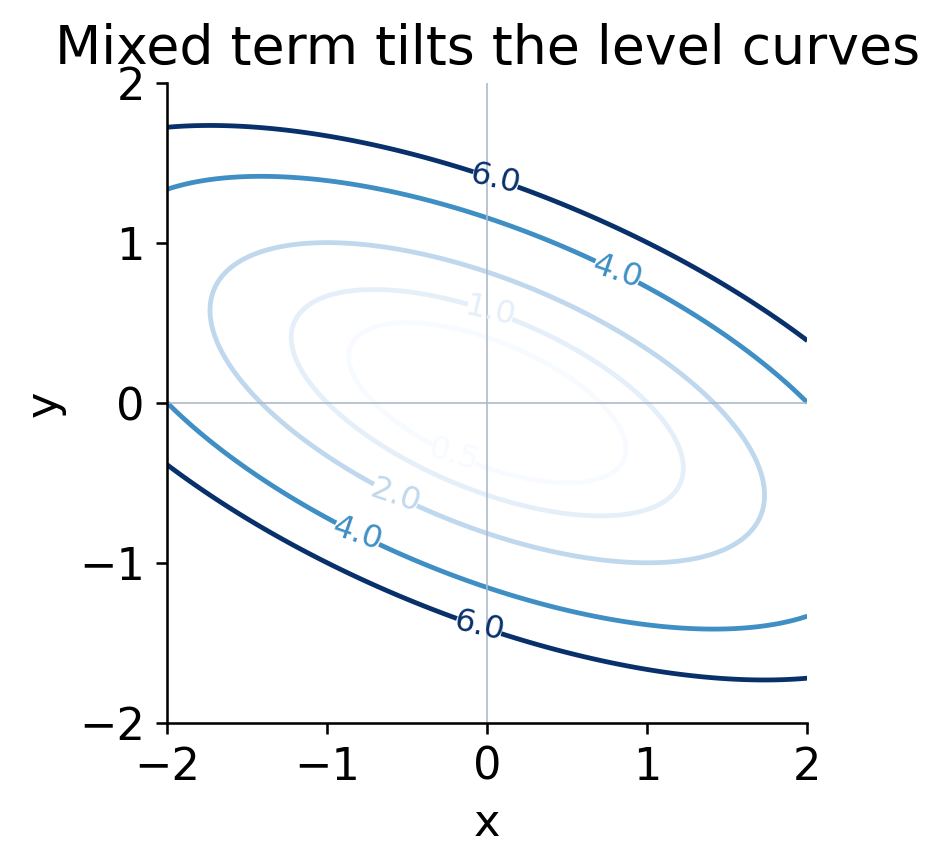
The extrema tests later in this unit formalise this connection. A vanishing first-order term alone does not establish whether the point is a minimum, maximum or saddle.
Worked Example 1.48: Complete the Square
For f=x²+2xy+3y², the origin is stationary and:
f = (x+y)²+2y²
This is positive for every nonzero input pair, so the origin is a strict minimum with value 0.
The Hessian entries are A=2, B=2 and C=6. Their determinant is:
AC−B² = (2)(6)−2² = 8>0
This is consistent with a positive-definite quadratic form.
Why the Mixed Term Matters
The function x²+4xy+y² has positive pure-square coefficients but takes negative values along y=−x. Positive coefficients of x² and y² alone therefore do not guarantee a minimum.
Degenerate Cases
If the quadratic term vanishes or is only semidefinite, higher-order terms may decide the shape. The functions x⁴+y⁴ and x⁴−y⁴ have the same zero Hessian at the origin but different behaviour.
Bridge to Optimisation: Taylor expansion explains the Hessian test: a definite leading quadratic term dominates a sufficiently small higher-order remainder. When that term is inconclusive, examine the function more directly.
30. Jacobian: A Derivative of a Transformation
A transformation assigns outputs u=u(x,y) and v=v(x,y). Its Jacobian matrix contains all four first partials; its Jacobian determinant is:
J = ∂(u,v)/∂(x,y) = uₓvᵧ−uᵧvₓ
The output order and input order are part of the notation. Interchanging one pair changes the sign of the determinant.

Matrix Versus Determinant
The matrix is the full linear derivative map. The determinant is one scalar derived from it. “Find the Jacobian” often means the determinant in first-year problems, but identify which object the question requests.
The Full Linearised Map
For small input increments h and k:
Δu ≈ uₓh+uᵧk
Δv ≈ vₓh+vᵧk
The matrix acts on the displacement. Its determinant is the signed area factor of this linear map. A scalar determinant alone does not retain every direction and stretching detail of the full derivative matrix.
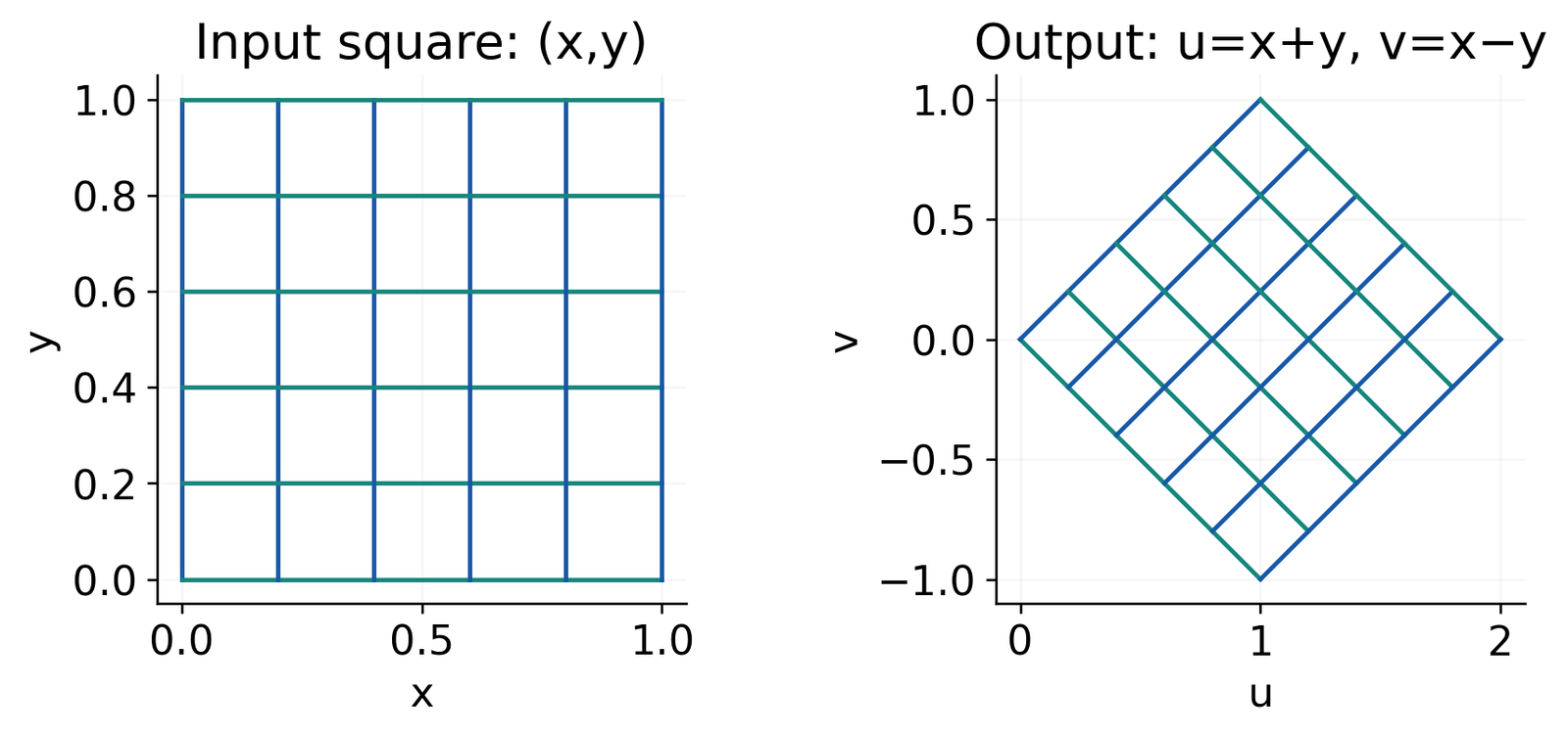
Worked Example 1.49: A Linear Jacobian
Let u=x+y and v=x−y:
- uₓ=1
- uᵧ=1
- vₓ=1
- vᵧ=−1
J = (1)(−1)−(1)(1) = −2
The magnitude is 2, while the negative sign indicates orientation reversal. These are different pieces of information.
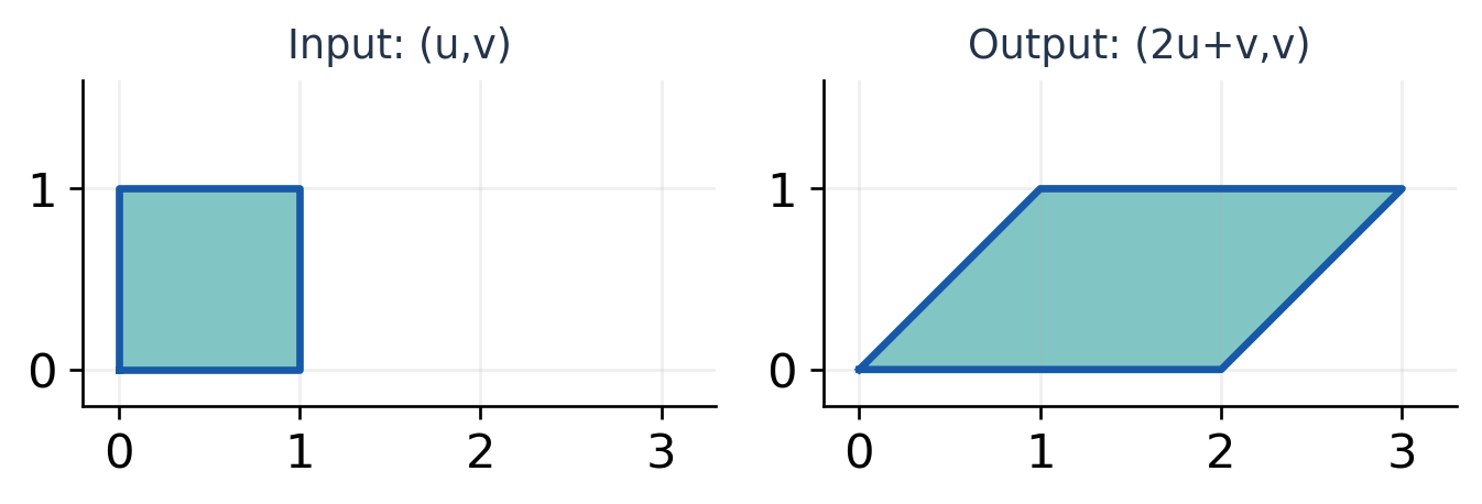
Local Area Interpretation
For a sufficiently small input parallelogram, the transformed area is approximately |J| times the original area at that point. In a nonlinear map, J can vary from point to point.
A Zero Determinant
J=0 means the linearised map is singular there. It does not alone establish every global property of the nonlinear map, and it does not automatically prove an identity relating the outputs throughout a region.
Order Check
For the same example, ∂(v,u)/∂(x,y)=+2. Swapping both input and output order returns the original sign.
Calculation Pattern: Write outputs in rows and inputs in columns, compute all partials in that order, then apply the determinant signs. A sign error often begins with an unnoticed order change.

31. Direct Jacobian Calculations
Worked Example 1.50: A Quadratic Transformation
Let u=x²−y² and v=2xy.
uₓ=2x, uᵧ=−2y, vₓ=2y, vᵧ=2x
The determinant is:
J = (2x)(2x)−(−2y)(2y) = 4(x²+y²)
At (1,1), J=8. It is nonzero away from the origin and zero at the origin.
What Nonzero Means Locally
Under the usual smoothness assumptions, a nonzero Jacobian determinant gives a locally differentiable inverse near the point. This is a local conclusion, not a guarantee that the map is one-to-one over its entire domain.
For this transformation, (x,y) and (−x,−y) give the same output. Its nonzero local determinant away from the origin does not remove that global two-to-one behaviour.
Worked Example 1.51: A Nonlinear Map with Positive Jacobian
Let u=eˣ cos y and v=eˣ sin y. The partials satisfy:
uₓ=u, uᵧ=−v, vₓ=v, vᵧ=u
Therefore:
J = u²+v² = e^(2x)>0
The map is locally nonsingular everywhere, but increasing y by 2π repeats the same output. This gives another explicit example where a nonzero Jacobian does not guarantee global one-to-one behaviour.
Worked Example 1.52: A Product and Ratio
Let u=xy and v=x/y on a domain with y≠0.
uₓ=y, uᵧ=x, vₓ=1/y, vᵧ=−x/y²
Therefore:
J = y(−x/y²)−x(1/y) = −2x/y
The determinant also vanishes where x=0, even though the original transformation is defined there if y≠0.
Domain Versus Invertibility
A formula may be defined at a point where its derivative map is singular. “Defined,” “nonzero Jacobian” and “globally invertible” should not be treated as equivalent statements.
Common Mistakes
Do not differentiate x/y in x as if y also varied unless the problem explicitly makes it a dependent variable. Here x and y are independent input coordinates.
Do not take the absolute value unless an area magnitude or another nonnegative quantity is requested. The signed Jacobian itself retains orientation information.
Check with a Point: At x=y=1, the derivatives give J=−2 directly. This simple substitution can help verify the sign of the simplified expression.
32. Polar-Coordinate Jacobian


For x=r cos θ and y=r sin θ, the input order is (r,θ) and output order is (x,y).
xᵣ=cos θ, x_θ=−r sin θ
yᵣ=sin θ, y_θ=r cos θ
The angle is in radians. The usual polar chart takes r≥0, with a locally chosen angular branch when an inverse is needed.
Worked Example 1.53: Calculate the Factor
Using the determinant:
∂(x,y)/∂(r,θ) = r cos²θ+r sin²θ = r
For r>0 on a smooth local inverse branch:
∂(r,θ)/∂(x,y) = 1/r
At r=0, the polar parametrisation is singular: all angle values describe the same origin. The inverse expression 1/r cannot be used there.
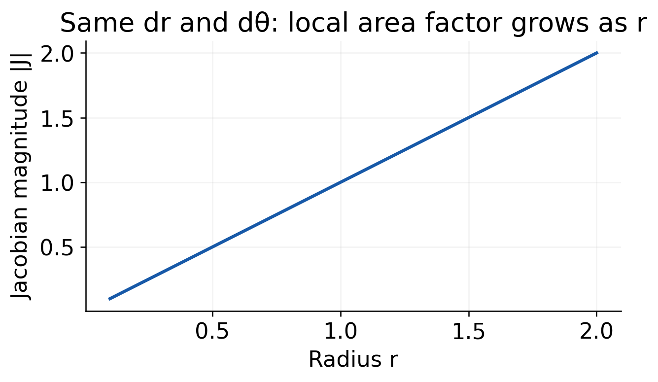
Geometric Explanation
A small radial change contributes length dr. A small angular change contributes approximately r dθ along a circle. Their local area product is r dr dθ, consistent with the Jacobian.
This explains the coordinate factor used in multiple integrals later. The present result is a local derivative calculation; changing an integral also requires transforming its domain and integrand.
Order Warning: ∂(y,x)/∂(r,θ)=−r. The familiar positive r factor assumes the stated output and input orders and a nonnegative radial coordinate.
33. Chain and Inverse Properties of Jacobians
For a smooth composite transformation (x,y)→(r,s)→(u,v), the determinant chain rule is:
∂(u,v)/∂(x,y) = [∂(u,v)/∂(r,s)]·[∂(r,s)/∂(x,y)]
When a smooth local inverse exists:
[∂(u,v)/∂(x,y)]·[∂(x,y)/∂(u,v)] = 1
The syllabus requests Jacobian properties without proof. Apply them with the correct evaluation points and a nonzero determinant for inverse use.
Worked Example 1.54: Inverse of a Linear Map
For u=x+y and v=x−y, J=−2. The inverse is:
x=(u+v)/2, y=(u−v)/2
Its determinant is −1/2. Their product is 1.
Worked Example 1.55: Reciprocal at a Specified Point
For u=x²+y² and v=x/y, on y≠0:
J = −2(x²+y²)/y²
At (1,1), J=−4. A suitable smooth local inverse therefore has determinant −1/4 at the corresponding output (u,v)=(2,1).
The inverse determinant is evaluated at the transformed point, not at an arbitrary output pair.
Worked Example 1.56: A Composite Map
Let r=x+y, s=x−y, followed by u=r²−s² and v=2rs.
The inner determinant is −2. The outer determinant is 4(r²+s²). Hence:
J = −8(r²+s²) = −16(x²+y²)
Independent Direct Check
The composite formulas simplify to u=4xy and v=2x²−2y². Thus:
J = (4y)(−4y)−(4x)(4x)
This again gives −16(x²+y²).
Evaluation Points Matter
The outer determinant must be evaluated at (r(x,y),s(x,y)), not at an unrelated numerical pair. The determinant notation is not a permission to cancel partial-derivative symbols as ordinary fractions.
Local Inverse Limitation
A nonzero determinant is a sufficient local condition under smoothness. Global inverse questions also depend on the domain and possible repeated outputs.
Efficient Method: Use the product property for a complicated composite transformation, then verify with direct differentiation when the simplified expressions are short enough.



34. Functional Dependence
Outputs are functionally dependent when a nontrivial relation Φ(u,v)=0 holds throughout a suitable region. Under appropriate smoothness and regularity, such a relation forces the two-output Jacobian to vanish there.

Worked Example 1.57: Identify the Relation
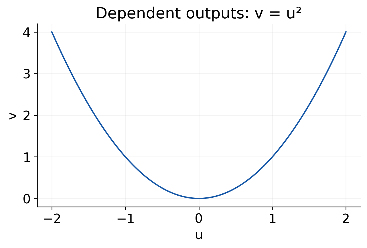
Let u=x²+y² and v=x⁴+2x²y²+y⁴. The second expression is u², so:
v−u² = 0
Also vₓ=2u uₓ and vᵧ=2u uᵧ, giving:
uₓvᵧ−uᵧvₓ = 0
The zero determinant follows from an explicit output relation, not from numerical coincidence at one point.
A Single Zero Is Not an Identity
For u=x² and v=y², J=4xy. It vanishes at the origin and along the coordinate axes, but the outputs can vary independently on a region where x and y are both positive.
Thus J=0 at one point does not prove that u and v obey one nontrivial regular relation throughout a neighbourhood.
Local Rank Interpretation
The Jacobian matrix describes the first-order output changes. A zero determinant means this first-order map fails to cover two independent output directions at that point.
A conclusion about full functional dependence requires additional conditions and a region-level statement. When an explicit relation can be found by algebra, exhibit it directly.
Common Exam Pattern
To show dependence, simplify the outputs and eliminate x and y where possible. Then verify the relation. If also asked for the Jacobian, calculate it in the stated order and connect its zero value with the dependence.
Do Not Overstate a Property
Introductory summaries sometimes state a zero-Jacobian rule without its local hypotheses. In an answer, distinguish an identically zero determinant in a suitable regular setting from a determinant that merely vanishes at isolated points.
Reliable Conclusion: An explicit nontrivial relation is the clearest evidence of dependence in elementary problems. A single zero numerical determinant is only a singular-point observation.
35. Jacobians in Three Variables
For u,v,w depending on x,y,z, place one output’s partial derivatives in each row and one input coordinate in each column. The determinant is written ∂(u,v,w)/∂(x,y,z).
The determinant chain rule and local inverse reciprocal rule extend to equal-dimensional transformations, with the same smoothness and nonzero-determinant conditions.
Worked Example 1.58: A Linear Three-Output Map
Let u=x+y, v=y+z and w=z+x. The derivative matrix is:
| Output | x Column | y Column | z Column |
|---|---|---|---|
| u | 1 | 1 | 0 |
| v | 0 | 1 | 1 |
| w | 1 | 0 | 1 |
Expanding along the first row:
J = 1(1)−1(−1)+0 = 2
The nonzero constant determinant confirms a nonsingular linear transformation.
Worked Example 1.59: Diagonal Transformation
For u=x², v=y² and w=z²:
J = (2x)(2y)(2z) = 8xyz
The determinant vanishes on the coordinate planes. On a positive-coordinate branch, the inverse uses positive square roots and has determinant 1/(8xyz) evaluated at the matching point. Choosing a branch matters because signs are lost when coordinates are squared.
Recover the Linear Inverse Explicitly
For the transformation in Example 1.58, add u+w−v to get 2x; similarly obtain:
x = (u−v+w)/2
y = (u+v−w)/2
z = (−u+v+w)/2
The inverse determinant is 1/2, consistent with the reciprocal property.
Check by Substitution
For (x,y,z)=(1,2,3), the outputs are (u,v,w)=(3,5,4). The inverse formulas return x=1, y=2 and z=3.
Row Order and Signs
Swapping two outputs changes the determinant sign. A cyclic reordering of three rows is an even permutation and preserves the sign. Do not reorder a matrix casually while keeping the same labelled determinant.
Implicit Systems
When outputs are defined by equations rather than explicit formulas, differentiating those equations gives a linear system for the required partials. Solve that system only where its coefficient Jacobian is nonsingular.
Practical Method: Write the dependency order, form the derivative matrix, use a clear determinant expansion and check any inverse by direct substitution. Most mistakes are organisation errors rather than difficult differentiation.
36. Local and Absolute Extrema
A local minimum has no smaller nearby domain values. An absolute minimum has no smaller value anywhere in the entire stated domain. Maxima reverse these inequalities.
At an interior local extremum of a differentiable function, all first partial derivatives vanish:
fₓ=0, fᵧ=0
These are necessary conditions, not sufficient ones.
A stationary point may be a minimum, maximum or saddle. Nondifferentiable points and boundary points can also be extrema and require separate examination.
Worked Example 1.60: A Direct Global Minimum
For f=x²+y², both partials vanish only at the origin. Since squares are nonnegative:
f(x,y) ≥ 0 = f(0,0)
Thus the origin is an absolute minimum. There is no absolute maximum on the whole plane because f grows without bound.
Why the Domain Matters
On a closed disk x²+y²≤1, the same function has minimum 0 at the origin and maximum 1 at every boundary point. On the open disk, the supremum is still 1 but it is not attained, so there is no maximum.

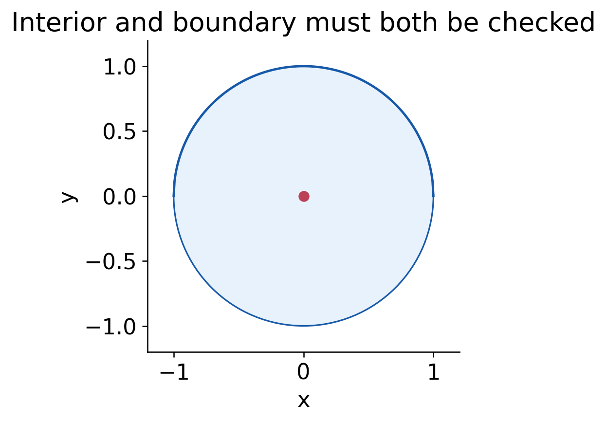
Extreme-Value Existence
A continuous function on a nonempty compact domain has an absolute maximum and minimum. This ensures existence, but it does not identify where those values occur.
A Complete Search
Find interior stationary points, examine nonsmooth points if present, analyse the boundary or constraints, and compare candidate values. If the domain is unbounded or open, check limiting behaviour as well.
Strict Versus Non-Strict
A strict minimum is strictly smaller than all other sufficiently nearby values. A non-strict minimum allows ties, such as a function that is constant along a line of minimisers.
Necessary-Condition Warning: Solving fₓ=fᵧ=0 finds smooth interior stationary candidates. It does not certify an optimum or automatically include every possible extremum on the domain.
37. The Two-Variable Hessian Test
For a C² function at a stationary point, write A=fₓₓ, B=fₓᵧ and C=fᵧᵧ, all evaluated there. Define:
D = AC−B²
| Condition | Conclusion |
|---|---|
| D>0 and A>0 | Strict local minimum |
| D>0 and A<0 | Strict local maximum |
| D<0 | Saddle point |
| D=0 | Test inconclusive |
The test uses the Hessian at the stationary point. Applying it where the gradient is nonzero does not give the stated extremum classification.
Why the Determinant Appears
The second-degree Taylor term is a quadratic form. D and the sign of A determine whether that form is positive definite, negative definite or indefinite in two variables.
Worked Example 1.61: A Negative-Definite Maximum
For g=5−x²−xy−2y², the only stationary point is the origin.
A=−2, B=−1 and C=−4 give D=7>0 with A<0, so the point is a strict local maximum of value 5.
The identity:
g = 5−(x+y/2)²−7y²/4
also shows that this is the unique absolute maximum on the plane.
Worked Example 1.62: Classify a Quadratic
Let f=x²+xy+2y². Its stationary equations are:
2x+y=0, x+4y=0
These give only (0,0).
The second derivatives are A=2, B=1 and C=4:
D = (2)(4)−1² = 7>0
Since A>0, the origin is a strict local minimum, with value 0. Completing the square also shows that it is global:
f = (x+y/2)²+7y²/4
Test Sequence
- Find first partials and solve the stationary equations.
- Compute second partials before substituting each candidate.
- Evaluate A, B, C and D at the candidate.
- State the local classification and function value.
- Check domain or global requirements separately if requested.
Inconclusive Means Unresolved
D=0 does not mean “no extrema.” It means this particular second-order test does not decide the question; use higher-order terms or direct sign analysis.
Worked Example 1.63: A Line of Minima
For f=(x+y)², both first partials vanish whenever x+y=0. The Hessian has A=B=C=2 and D=0.
Nevertheless f≥0 everywhere, with equality along the whole line y=−x. Every point on that line is a non-strict absolute minimiser.
The zero determinant correctly warns that the strict second-order classification does not decide the full geometry.


38. A Shifted Quadratic Minimum
Worked Example 1.64: Include a Mixed Term
Find and classify stationary points of:
f = x²+xy+y²−3x−3y
The first partial equations are:
2x+y−3=0
x+2y−3=0
Subtracting gives x=y. Substitution gives x=y=1.
The function value is:
f(1,1) = 1+1+1−3−3 = −3
The Hessian entries are A=2, B=1 and C=2. Thus D=3>0 and A>0, establishing a strict local minimum.
A Global Certificate
With h=x−1 and k=y−1:
f = −3+h²+hk+k²
The remaining quadratic is positive for nonzero (h,k), so this is the unique absolute minimum on the plane.
Use a Positive Quadratic Form
The inequality |hk|≤(h²+k²)/2 gives:
h²+hk+k² ≥ ½(h²+k²)
Hence the difference f+3 is strictly positive away from (1,1). This direct argument establishes global behaviour that a local Hessian test alone does not automatically claim.


Maximum of a Negative Quadratic
Changing the overall sign of a positive-definite quadratic gives a strict maximum at its centre. For example, −x²−2y² has maximum 0 at the origin and decreases without bound away from it.
What Changes Under a Constant Shift?
Adding a constant changes every function value equally but does not change first or second derivatives. It therefore shifts the extremum value without moving its location or changing its local type.
Distinguish Proof Levels: The Hessian test provides a local classification. A completed-square representation or another global inequality can establish a global minimum on the full domain.
39. Saddles and Degenerate Tests
Worked Example 1.65: A Saddle
For f=x²−y², the origin is stationary. A=2, B=0 and C=−2:
D = −4<0
The point is a saddle.
Along y=0, f=x²≥0, while along x=0, f=−y²≤0. Arbitrarily close points therefore lie both above and below the origin’s value.

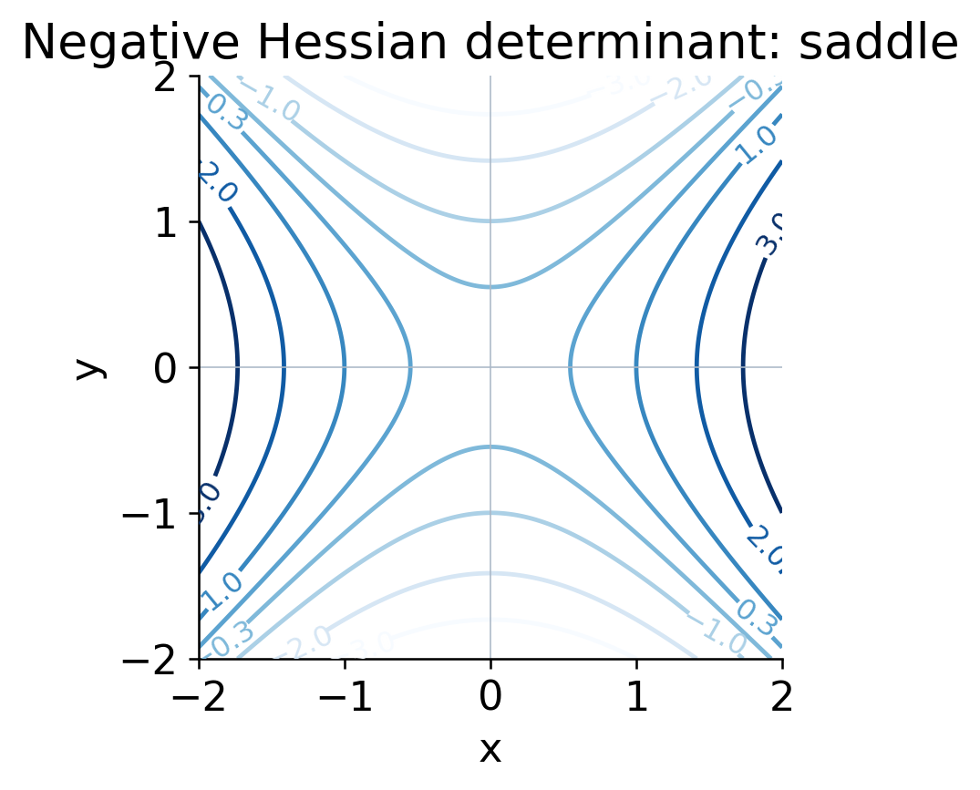
A saddle is not classified as an extremum merely because both first derivatives vanish.
Worked Example 1.66: Same Hessian, Different Outcome
At the origin, both f=x⁴+y⁴ and g=x⁴−y⁴ have zero first and second partials, so D=0 for each.
For f, all values are nonnegative and equality occurs only at the origin. It has a strict absolute minimum there.
For g, the x axis gives positive values and the y axis negative values near the origin. It has a saddle.


Final Test: When D=0, inspect the actual function, its first nonzero higher-order terms, or suitable sign-changing paths. Do not replace “inconclusive” with an unsupported classification.
40. More Than One Critical Point
Worked Example 1.67: A Cubic Surface
Let f=x³+y³−3xy. The first partials give:
fₓ = 3x²−3y = 0
fᵧ = 3y²−3x = 0
Thus y=x² and x=y². Substitution gives x=x⁴, whose real solutions are x=0 and x=1. The critical points are (0,0) and (1,1).
The Hessian entries are A=6x, B=−3 and C=6y.
At (0,0), D=−9, so the point is a saddle.
At (1,1), D=36−9=27 and A=6>0, so it is a strict local minimum with value −1.
Do not stop after finding one stationary pair: nonlinear equations can produce several candidates.
Local Does Not Mean Global

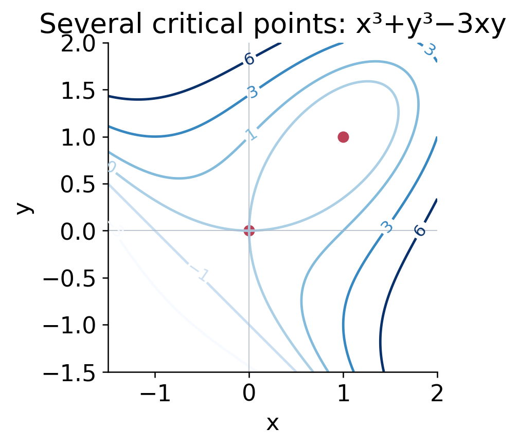
Along x=y=−t for positive large t:
f(−t,−t) = −2t³−3t² → −∞
Thus the local minimum value −1 is not an absolute minimum on the whole plane. The function has no global lower bound there.
Solving Without Losing Candidates
If a stationary equation contains a product, do not divide by a variable before checking the zero case. Otherwise a candidate such as the origin can disappear from the calculation.
Compare Candidate Values Only When Appropriate
For a compact constrained problem, comparison can identify global extremes after all candidates and boundaries are included. For an unbounded domain, candidate comparison alone cannot rule out values tending to infinity or minus infinity.
Organisation Trick: Make a small candidate table containing location, A, B, C, D, local type and function value. Then add a separate global-behaviour statement if the question asks for it.
Candidate Table and Upper Behaviour
| Point | D | Type and Value |
|---|---|---|
| (0,0) | −9 | Saddle, f=0 |
| (1,1) | 27 | Local minimum, f=−1 |
Along x=y=t with t→+∞:
f = 2t³−3t² → +∞
Together with the negative-direction calculation, this establishes that the whole-plane function has neither an absolute maximum nor an absolute minimum.

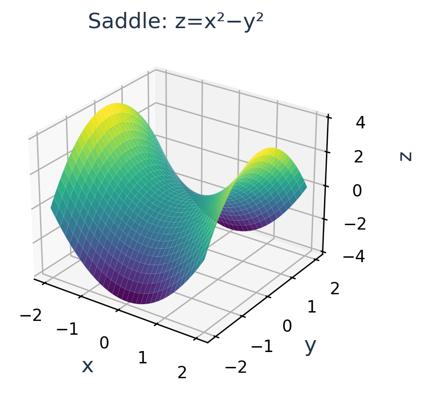
41. Extrema in Several Variables
For f(x₁,…,xₙ), a smooth interior extremum must satisfy ∇f=0. The Hessian is the symmetric matrix of second partials under the usual C² assumptions.
A positive-definite Hessian gives a strict local minimum. A negative-definite Hessian gives a strict local maximum. An indefinite Hessian gives a saddle. A semidefinite or singular case can require further analysis.
Leading-Minor Test
For a symmetric Hessian, positivity of all leading principal minors is a criterion for positive definiteness. Negative definiteness uses alternating signs of those minors, starting negative.
A determinant alone is not enough in three or more variables. The two-variable A,D rule should not be copied as a complete higher-dimensional test.
Practical Scope
For diagonal or easily completed-square forms, direct sign analysis is often simpler than a long determinant calculation. State the criterion used rather than memorising disconnected signs.
Worked Example 1.68: Three-Variable Minimum
Let:
f = (x−1)²+2(y+2)²+3(z−3)²
The stationary point is (1,−2,3).
The Hessian is diagonal with entries 2,4,6. Its leading principal minors are:
2, 2·4=8, 2·4·6=48
They are all positive. The point is a strict local minimum. Since every squared term is nonnegative, it is also the unique absolute minimum, with value 0.
Worked Example 1.69: A Positive Determinant Can Mislead
For g=−x²−y²+z², the Hessian diagonal entries are −2,−2,2. Its determinant is +8, but the function increases along the z axis and decreases along the x axis.
The origin is therefore a saddle, not a minimum. The Hessian is indefinite despite its positive determinant.
Global Certificate
For a positive weighted sum of squares, equality conditions identify the minimiser directly. This gives both the location and uniqueness without relying only on a local test.
Higher-Dimensional Rule: Check definiteness, not just determinant sign. When the quadratic form has both positive and negative directions, the stationary point is a saddle.
Worked Example 1.70: A Three-Variable Maximum
For f=5−x²−2y²−3z², the origin is stationary. The Hessian is diagonal with entries −2,−4,−6, and its leading principal minors are:
−2, +8, −48
Their alternating signs give negative definiteness. The origin is a strict local maximum, and the nonpositive square terms show it is also the unique absolute maximum, with value 5.
42. Unconstrained Model Optimisation
A loss function assigns a numerical mismatch to model parameters. Multivariable calculus finds stationary candidates and determines whether they minimise the specified loss.
Worked Example 1.71: Fit Two Data Points
Use the linear model predicted value wx+b for observations (0,1) and (1,3). Define a simple half-sum squared loss:
L(w,b) = ½[(b−1)²+(w+b−3)²]
The derivatives are:
L_w = w+b−3
L_b = w+2b−4
Solving them simultaneously gives b=1 and w=2. Both residuals then vanish, so L=0.
This is a mathematical toy dataset that makes the optimisation steps visible. It is not a claim about the performance of a trained real-world model.
Classify the Solution
The second partials are:
L_ww=1, L_wb=1, L_bb=2
The Hessian determinant is 1, and the first leading entry is positive.
The stationary point is a strict local minimum. More strongly, the loss is a sum of nonnegative squares, so zero is the global minimum. The two linear residual equations identify a unique parameter pair here.
Why Two Derivatives Are Needed
The slope w and intercept b influence the same prediction at x=1. Optimising one parameter while arbitrarily freezing the other generally does not solve the joint problem.
A Complete Application Answer
Define the objective, state the adjustable variables, differentiate, solve the stationary equations, classify the solution and interpret it in the original model.
What Calculus Does Not Guarantee
A small training loss on two observations does not establish generalisation to new observations. The present exercise studies the mathematical minimisation of the stated objective, not statistical model validation.
Constraint Distinction
If a parameter is required to be nonnegative or a resource sum is fixed, the feasible domain changes. An unconstrained stationary point outside that domain is not an admissible answer.
CSE Connection: Gradients locate parameter directions and stationary points; curvature helps classify the objective. Always connect the calculus result back to the exact model and domain given in the question.
43. Lagrange Multipliers
To optimise f subject to a smooth equality constraint g=c, interior constrained extrema at regular constraint points satisfy:
∇f = λ∇g, g=c
The regularity condition is ∇g≠0 at the candidate. It ensures that the constraint is locally a smooth curve or surface. Boundary restrictions and singular constraint points still require separate checks.
One consistent convention is to define the Lagrangian:
ℒ = f−λ(g−c)
Setting its x and y partials to zero gives fₓ=λgₓ and fᵧ=λgᵧ, together with the original constraint.
Why Gradients Become Parallel
At a smooth constrained extremum, feasible tangent motion has no first-order change in the objective. Both gradients are normal to the feasible tangent direction, giving the parallel-gradient condition.
First-Order Tangent Explanation
Along a smooth feasible path r(t) through a constrained optimum, the chain rule gives:
∇g·r′(t)=0
∇f·r′(t)=0
In the plane, a nonzero constraint gradient identifies a normal to the feasible tangent. The objective gradient is also normal there, so the gradients are parallel. This explains the multiplier condition and why the regularity hypothesis is needed.
Joseph-Louis Lagrange


Worked Example 1.72: Minimum on a Line
Minimise f=x²+y² subject to x+y=6. The gradient equations give:
2x=λ, 2y=λ
So x=y. The constraint gives x=y=3.
The value is 18. Substitution into the line gives x²+(6−x)², a positive quadratic with its minimum at x=3, confirming the global constrained minimum.
There is no constrained maximum on the unrestricted line, because the objective grows without bound.
Method Boundary: A Lagrange solution is a candidate subject to its hypotheses. Compare objective values and check the feasible domain before claiming a global extremum.
44. Extrema on a Circle
Worked Example 1.73: Linear Objective, Circular Constraint
Optimise f=x+y subject to x²+y²=1. Use g=x²+y².
1=2λx, 1=2λy
The equations imply λ≠0 and x=y. The constraint then gives:
x=y=1/√2, or x=y=−1/√2
At the positive pair, f=√2; at the negative pair, f=−√2.
The circle is compact and f is continuous. Its gradient constraint is nonzero everywhere on the circle, and these are the complete Lagrange candidates. Thus the values are the absolute constrained maximum and minimum, respectively.
Geometry of the Condition

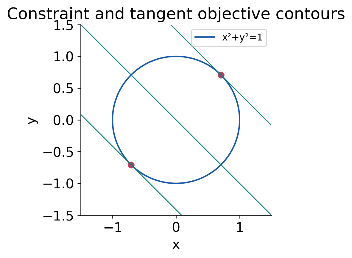
Check Without Multipliers
The inequality (x+y)²≤2(x²+y²) gives |x+y|≤√2 on the circle. Equality requires x=y, confirming the same two points.
What Not to Divide Away
The equations 1=2λx and 1=2λy show that x and y cannot be zero at a candidate. In a different problem, a variable might be zero; dividing by it without a separate case could lose valid candidates.
Constraint Versus Domain Boundary
The circle is itself the equality constraint. There is no additional endpoint to check on this smooth closed curve. Extra restrictions such as x≥0 would change the feasible set and could create boundary candidates.
Global Conclusion: State both locations and objective values. “λ found” is not the optimisation answer; the multiplier is a tool for identifying and interpreting feasible candidates.
Worked Example 1.74: Product on a Circle
Optimise f=xy on x²+y²=1. The equations are:
y=2λx, x=2λy
Neither coordinate can be zero at a candidate; otherwise the equations contradict the constraint.
Thus 4λ²=1.
- For λ=1/2, y=x and the product is 1/2.
- For λ=−1/2, y=−x and the product is −1/2.
The bound 2|xy|≤x²+y²=1 certifies the global values. The maximum occurs at the two equal-sign pairs (±1/√2,±1/√2), and the minimum at the two opposite-sign pairs. All four candidates matter, not just one point for each value.

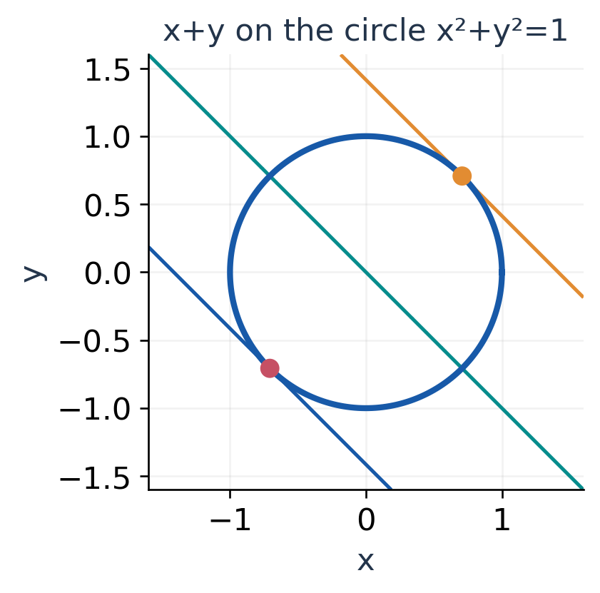
45. Resource Allocation and Nonnegativity
Worked Example 1.75: Maximise a Product
Suppose two nonnegative resource quantities satisfy x+y=10, and the model benefit is f=xy. The units and model are abstract; the task is to optimise the stated product.
The multiplier equations are:
y=λ, x=λ, x+y=10
Thus x=y=5, and the benefit is 25.
To check the global result, substitute y=10−x:
f = x(10−x) = 25−(x−5)²
For 0≤x≤10, the maximum is clearly 25. At either endpoint the product is 0, giving the minimum on the closed nonnegative feasible segment.
The Feasible Set Changes the Answer

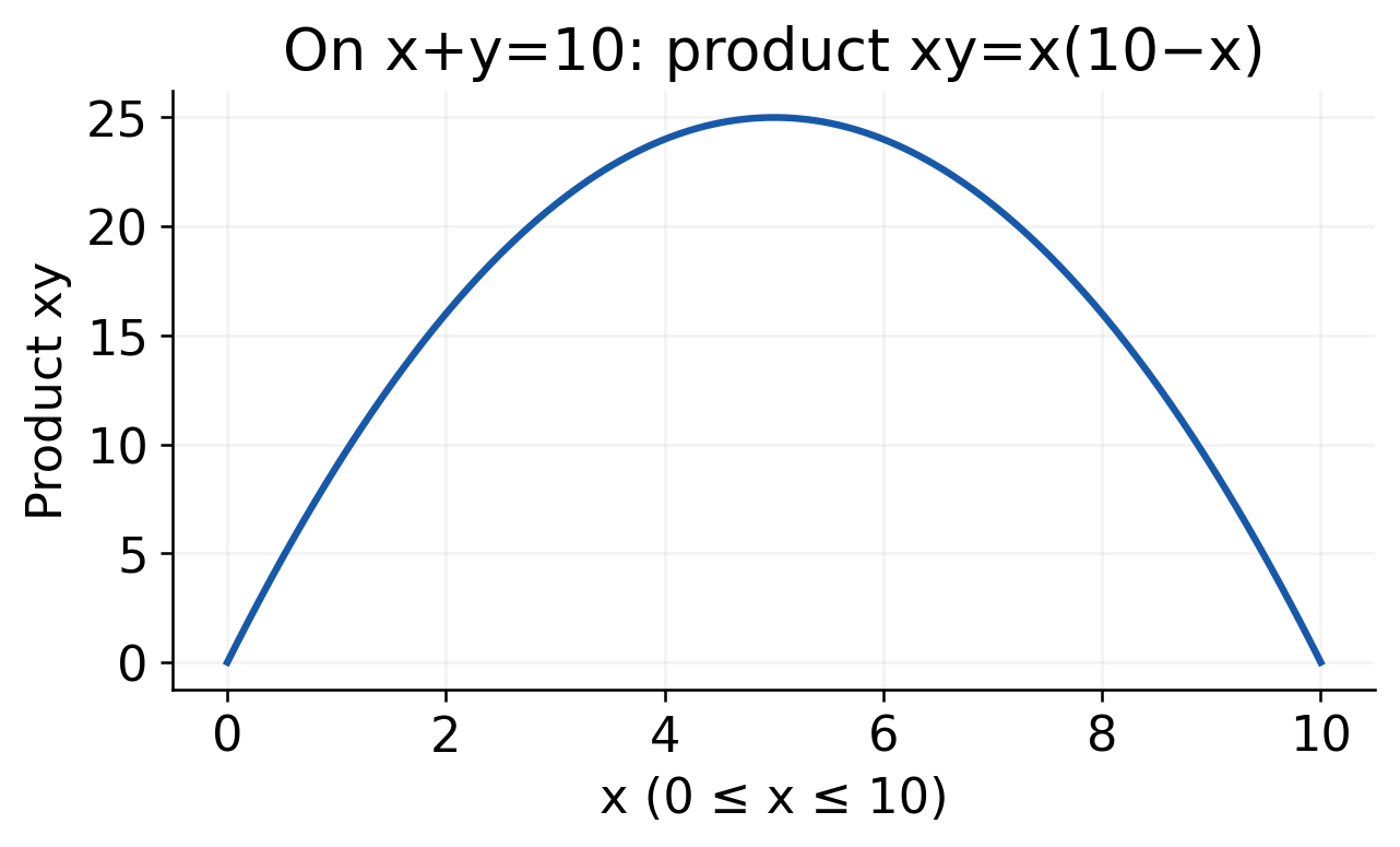
If the domain required x>0 and y>0 strictly, the maximum would still occur at (5,5), but the minimum 0 would not be attained. It would only be an infimum approached near either endpoint.
Why Boundary Checks Matter
The smooth Lagrange condition finds the interior constrained candidate. Nonnegative resource restrictions also create endpoints, which must be included when searching for absolute extrema.
Model Interpretation
Equal allocation is optimal here because the objective and constraint are symmetric. If the benefit weights, costs or feasible restrictions change, the optimal split may no longer be equal.
Short Proof Check
Using (x−y)²≥0 and x+y=10 gives xy≤25. This confirms the multiplier result and shows why equality requires x=y.
Application Habit: State whether quantities are positive, nonnegative or unrestricted. The same algebraic constraint can have different minimum and maximum conclusions under those different domains.
Worked Example 1.76: Unequal Resource Costs
Maximise xy with x,y≥0 and 2x+y=12. The multiplier equations give:
y=2λ, x=λ
So y=2x. Therefore x=3, y=6, and the maximum product is 18.
Directly:
xy = x(12−2x) = 18−2(x−3)²
on 0≤x≤6. The minimum is zero at the endpoints.
Unequal cost coefficients make the optimal quantities unequal even though the product objective is symmetric.
46. Lagrange Multipliers in Three Variables
For one smooth constraint g(x,y,z)=c, the regular-point condition becomes:
fₓ=λgₓ, fᵧ=λgᵧ, f_z=λg_z
together with the constraint.
Worked Example 1.77: Product Under a Fixed Sum
Maximise xyz for x,y,z≥0 and x+y+z=12. For positive interior candidates:
yz=λ, xz=λ, xy=λ
Because the coordinates are positive, dividing paired equations gives x=y=z. The constraint gives x=y=z=4, with product 64.
If any coordinate is zero, the product is zero. Continuity on the closed bounded feasible simplex guarantees extrema, so the positive interior candidate gives the absolute maximum. The minimum 0 occurs on the boundary.
Visualise the Feasible Region

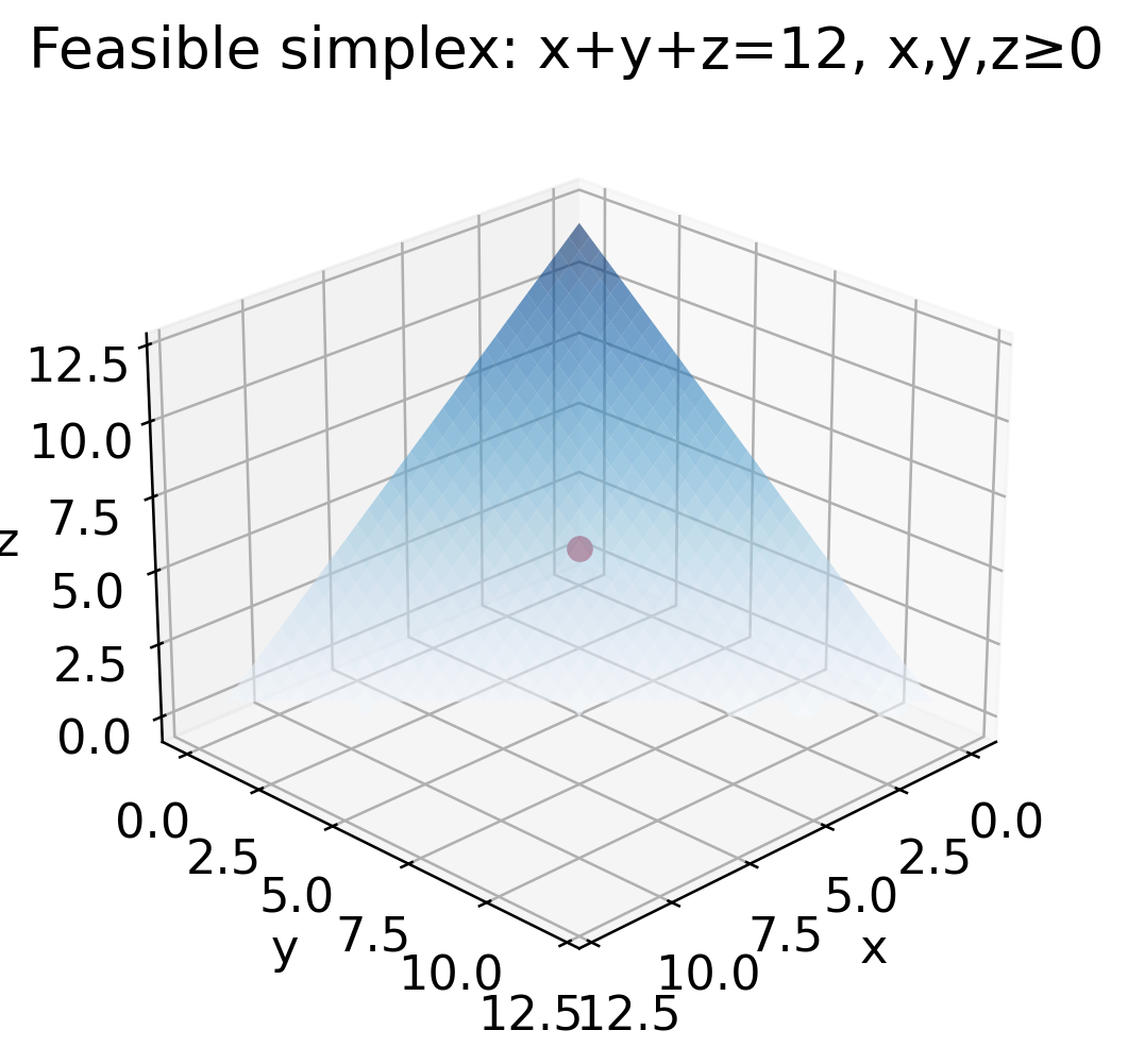
Worked Example 1.78: Minimum Squared Norm
Minimise x²+y²+z² subject to x+y+z=6, with unrestricted real coordinates.
The equations 2x=λ, 2y=λ and 2z=λ give x=y=z=2. The minimum value is 12.
A direct inequality also gives:
x²+y²+z² ≥ (x+y+z)²/3 = 12
There is no maximum on the unrestricted plane. If the coordinates were additionally nonnegative, the feasible triangle would instead have maximum 36 at its vertices.
Dimension Check: In three variables with one constraint, there are usually four unknowns including λ and four equations. Do not omit the original constraint after writing the gradient equations.
Worked Example 1.79: Weighted Squared Norm
Minimise x²+2y²+3z² subject to x+y+z=6. The multiplier equations give:
2x=λ, 4y=λ, 6z=λ
Hence:
λ(1/2+1/4+1/6) = 6
Thus λ=72/11, and the coordinates are:
(36/11,18/11,12/11)
The minimum value is 216/11.
A global certificate is the weighted inequality:
(x+y+z)² ≤ (x²+2y²+3z²)(1+1/2+1/3)
It gives the same lower bound 216/11, with equality at the multiplier solution.
47. Singular Constraints and Boundaries
The standard Lagrange theorem assumes a regular constraint gradient. At a singular point, the method can miss a genuine constrained extremum.
Worked Example 1.80: A Singular Feasible Set
Minimise f=x subject to x²+y²=0 over the reals. The only feasible point is (0,0), so it is both an absolute minimum and maximum, with value 0.
But ∇g=(2x,2y)=(0,0) there. The multiplier equation would demand:
(1,0) = λ(0,0)
which has no solution. This does not disprove the extremum; it shows that the regular-point theorem does not apply.
Practical Lesson
Before using multipliers, inspect whether the constraint gradient can vanish on the feasible set. Examine those points separately instead of dividing by a quantity that is zero there.
Worked Example 1.81: An Extremum on a Disk
For f=x on x²+y²≤1, there is no interior stationary point because fₓ=1.
Nevertheless:
- Maximum = 1 at (1,0)
- Minimum = −1 at (−1,0)
The boundary can be analysed by the equality constraint x²+y²=1 or by the simple bound −1≤x≤1.
Why an Inequality Is Different
An inequality domain has an interior and a boundary. Ordinary equality multipliers on the boundary are one useful part of the search, but they do not replace the interior and singular-point checks.
The full theory of inequality optimisation is broader than the basic multiplier method in this unit. Elementary domain decomposition is enough for the present examples.
Candidate Checklist
- Smooth interior stationary points.
- Equality-constrained regular candidates.
- Singular constraint points.
- Endpoints or additional nonnegativity boundaries.
- Limiting behaviour on open or unbounded domains.
Completeness Rule: A convincing optimisation answer explains why its candidate list is complete for the stated domain. Solving only the regular multiplier equations may leave out the actual answer.
48. Approximation of Changes and Errors
For a differentiable f near (a,b), small input changes h and k produce a first-order output estimate:
Δf ≈ df = fₓ(a,b)h+fᵧ(a,b)k
The signs matter for an estimated change. Positive and negative contributions can partly cancel. If only maximum input-error magnitudes are known, a first-order worst-case estimate uses absolute contributions instead:
E_lin = |fₓ|εₓ+|fᵧ|εᵧ
This is a linearised estimate. A rigorous finite-error bound needs derivative control over the whole uncertainty region or an exact monotonicity argument.
Distinguish Error Types
Absolute error has the output’s units. Relative error divides by a nonzero reference output magnitude. Percentage error is 100 times the relative error.
Worked Example 1.82: Rectangular Area
Let A=xy with x=10 and y=5. Suppose the measured changes are h=0.02 and k=0.01.
The partials at the reference point are Aₓ=5 and Aᵧ=10. Therefore:
dA = 5(0.02)+10(0.01) = 0.20
The estimated new area is 50.20. The exact value is:
(10.02)(5.01) = 50.2002
The neglected term is hk=0.0002, because the exact increment is yh+xk+hk.

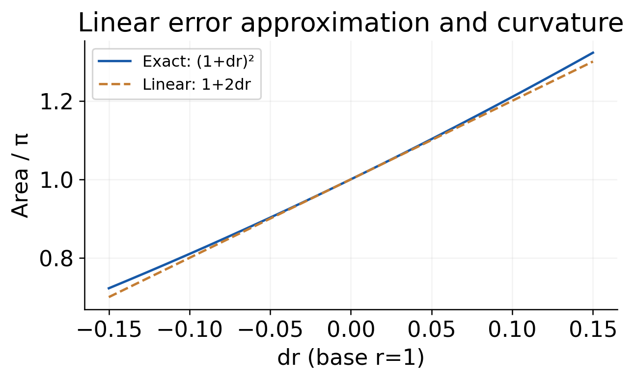
Interpretation
The approximation is close because the increments are small relative to the reference dimensions. Keeping the product hk would make this particular area calculation exact, but the differential alone is only first order.
Error Habit: Write the nominal point, signed changes or uncertainty magnitudes, the derivatives at that point, and the approximation symbol. Avoid presenting a first-order estimate as an exact finite change.
Worked Example 1.83: An Exact Differential Change
For f=3x−2y+7, let h=0.02 and k=−0.01.
df = 3h−2k = 0.08
Because the function is affine, the exact finite change is also 0.08 for any base point. This contrasts with the area example, where the product term hk survives beyond first order.
49. Relative and Percentage Errors
For f=Cxᵃyᵇ with suitable positive inputs and nonzero output, logarithmic differentiation gives:
df/f = a(dx/x)+b(dy/y)
A first-order worst-case relative-error estimate is:
|Δf|/|f| ≈ |a|εₓ/|x|+|b|εᵧ/|y|
The right side is an estimate based on local derivatives, not an automatic exact error bound for finite uncertainties.
Worked Example 1.84: A Cylinder
Let V=πr²h, with nominal r=3, h=5, radius uncertainty 0.01 and height uncertainty 0.02 in consistent length units.
The linearised magnitude relation gives:
|dV|/V ≤ 2(0.01/3)+0.02/5
The first-order estimate is 0.0106667, or about 1.067%.
Worked Example 1.85: Negative Exponent and Signed Change
Let f=x²/y at x=4, y=2, with uncertainty magnitudes 0.02 and 0.01.
The first-order worst-case relative estimate is:
2(0.02/4)+0.01/2 = 0.015
Thus it is 1.5%, or 0.12 in absolute output units because f=8.
If both signed input changes are positive, the linear relative change instead subtracts the denominator contribution and is 0.5%, giving df=0.04.
A possible signed change and a worst-case estimate are different answers.
Convert Back to Absolute Error
For the cylinder, the nominal volume is V=45π. The corresponding first-order absolute-error estimate is:
45π(0.0106667) = 0.48π ≈ 1.508

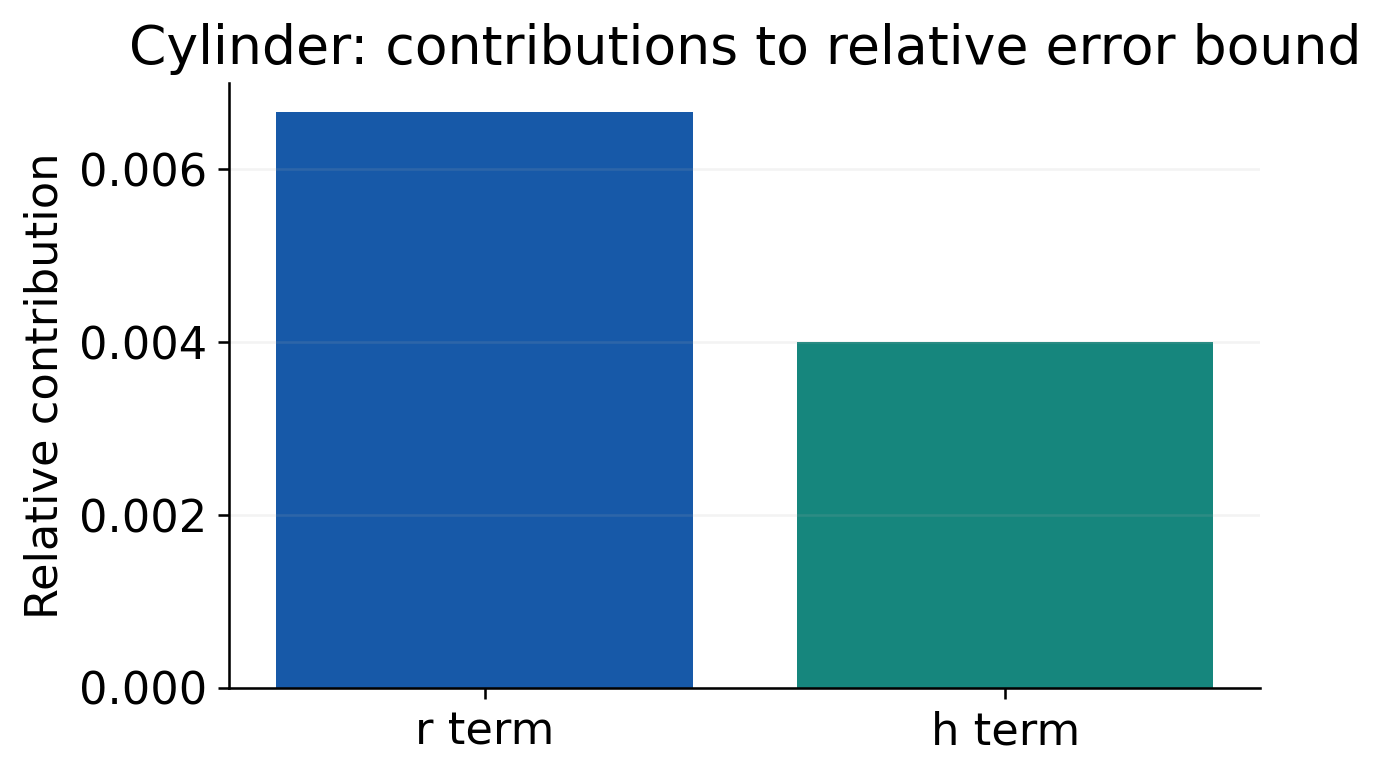
Why Radius Matters Twice
The area of the circular section depends on r², so a small relative radius change has approximately twice that relative effect on volume. The height enters to the first power.
Negative Exponents
For f=x²/y, the signed differential is df/f=2dx/x−dy/y. In a worst-case magnitude estimate, the two possible contributions add as positive magnitudes.
Reference Output
Relative error is problematic when the nominal output is zero or very close to zero. An absolute-error description may then be more informative.
Percentage Conversion: A relative error 0.0106667 corresponds to 1.06667%, not 0.0106667%. Multiply the dimensionless fraction by 100 only at the final step.
50. Signed Cancellation and Rigorous Bounds
First-order changes can cancel even when the exact change is nonzero. This does not invalidate differentials; it means the neglected higher-order terms become relatively important.
Worked Example 1.86: Cancellation in Area
Let A=xy at (20,10), with h=0.10 and k=−0.05.
dA = 10(0.10)+20(−0.05) = 0
The exact change is:
ΔA = dA+hk = −0.005
Thus the linear estimate predicts zero change, while the exact area decreases slightly. The input changes were coordinated so that the first-order terms cancelled.
Statistical Uncertainty Is Another Model
A worst-case magnitude estimate adds contributions. A statistical variance calculation uses assumptions about distributions and correlations. Do not replace one by the other without the required probabilistic information.
Worked Example 1.87: Check an Exact Worst Case
For the preceding cylinder r=3±0.01 and h=5±0.02 with positive dimensions, V increases with each input. The largest volume is therefore at r=3.01, h=5.02.
V_max = π(3.01)²(5.02) = 45.481702π
The exact upper deviation is 0.481702π≈1.5133, slightly larger than the first-order estimate 0.48π.
The smallest volume is 44.521698π, giving a lower deviation magnitude 0.478302π. The two finite deviations are not exactly symmetric.
A Derivative-Based Rigorous Bound
If |fₓ|≤Mₓ and |fᵧ|≤Mᵧ throughout a convex uncertainty region, integrate the derivative along the line segment between the nominal and perturbed points. This gives:
|Δf| ≤ Mₓ|h|+Mᵧ|k|
Using derivatives only at the nominal point gives the local estimate; using valid suprema over the whole region gives a genuine bound under the stated assumptions.
Precision Language: Say “first-order estimate” for nominal differential propagation. Reserve “guaranteed bound” for a justified interval-wide or exact argument.
Worked Example 1.88: A Guaranteed Rectangle Bound
For A=xy on the box:
- 9.98≤x≤10.02
- 4.99≤y≤5.01
the derivative bounds are Mₓ=5.01 and Mᵧ=10.02.
With |h|≤0.02 and |k|≤0.01:
|ΔA| ≤ 5.01(0.02)+10.02(0.01) = 0.2004
This is a valid finite-change bound over the box. It is slightly larger than the exact upper deviation 0.2002 and the nominal differential estimate 0.20.
51. Gradient-Based Model Tuning
The gradient ∇L points in the direction of steepest first-order increase under the usual Euclidean input metric. A small step in the negative-gradient direction is a natural local strategy for reducing a differentiable loss.
Worked Example 1.89: One Gradient Step
Take:
L = (w₁−2)²+2(w₂+1)²
Its gradient is:
∇L = (2(w₁−2),4(w₂+1))
At (0,0), the gradient is (−4,4) and L=6. With step size α=0.1:
(w₁,w₂)_new = (0,0)−0.1(−4,4)
The new point is (0.4,−0.4), with loss 3.28.

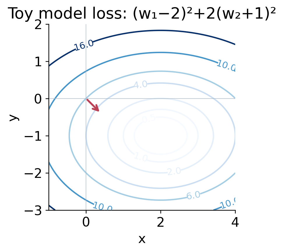
Step Size Is Part of the Method
With α=1 from the same starting point, the update gives (4,−4), whose loss is 22, larger than the initial value 6.

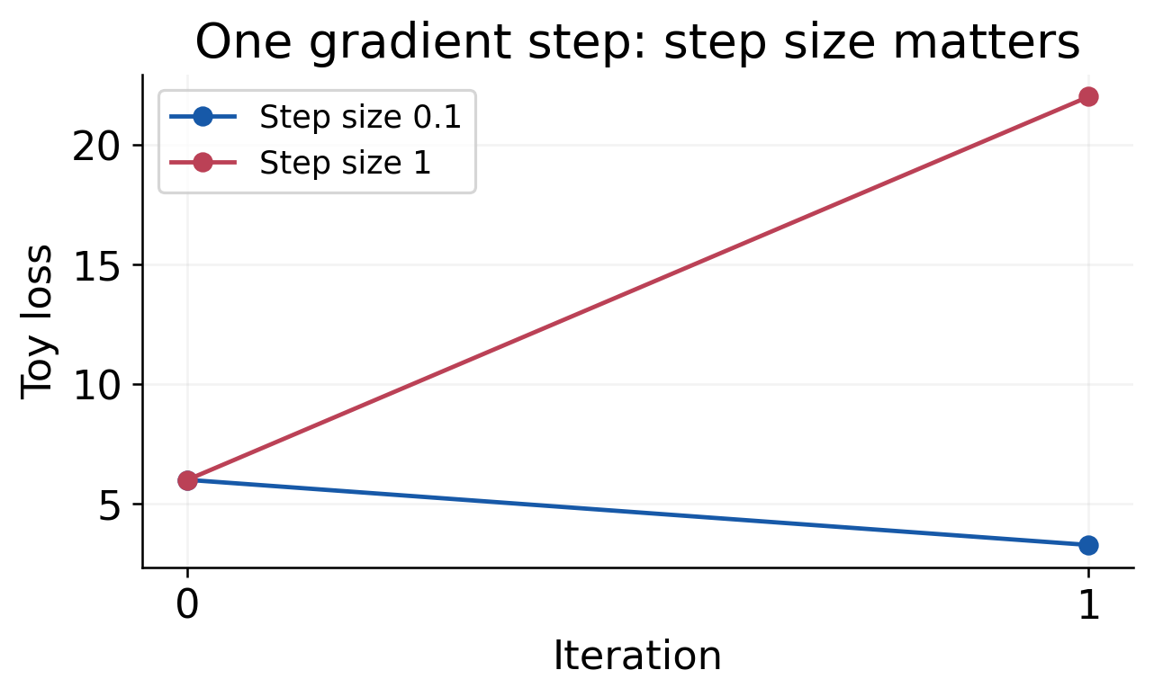
Exact Convergence Check for This Toy Model
The coordinate errors relative to the minimiser evolve by factors 1−2α and 1−4α. Requiring both magnitudes to be less than 1 gives:
0<α<1/2
for convergence of this fixed-step iteration.
This interval belongs to the particular quadratic and step convention. It is not a universal learning-rate rule.
Why This Fits the Calculus Syllabus
First partials give parameter sensitivities. The Hessian describes local curvature, explaining why a step that is small in one direction can be too large in another.
Model Scope: The example teaches differentiation and optimisation of an explicit function. Actual neural-network training introduces further issues beyond this elementary calculation.

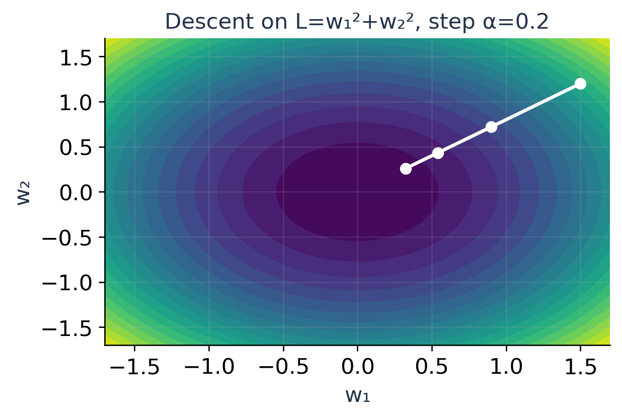
52. Cloud Capacity: A Constrained Cost Model
Suppose two positive capacities x and y share a fixed budget x+y=18. Consider the illustrative cost:
C(x,y) = 100/x+64/y
The constants and units are abstract model inputs. The formula is not a benchmark for any named cloud provider or real server system.
Worked Example 1.90: Allocate the Budget
Use ∇C=λ∇(x+y). Then:
−100/x²=λ
−64/y²=λ
Since x,y>0, equality gives 10/x=8/y, so x:y=10:8. The sum constraint gives:
x=10, y=8
The minimum model cost is:
C = 100/10+64/8 = 18
The optimum is unequal because the two inverse-cost weights are unequal.
Check That It Is a Minimum
Substitute y=18−x for 0<x<18. The second derivative is:
C″(x) = 200/x³+128/(18−x)³>0
Thus the restricted cost is strictly convex. It also tends to infinity at either end of the feasible open interval, confirming the unique global minimum.

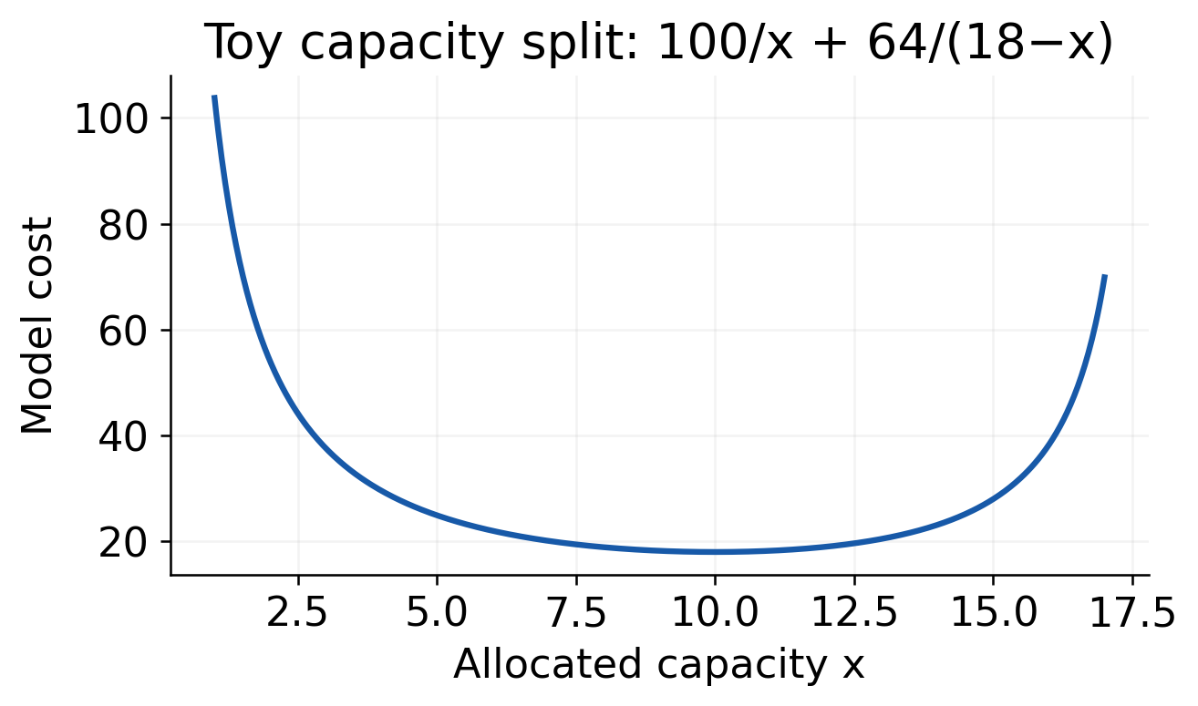
Multiplier Interpretation
Using the convention Lagrangian C−λ(x+y−18), the multiplier at the solution is λ=−1. Its sign is consistent with extra budget locally reducing the optimised cost. Other sign conventions change the multiplier sign.
Applications Need Assumptions
Before using a calculus model in resource allocation, identify the cost, feasible resources and whether the assumed relationship is appropriate. The mathematical optimum is only as relevant as that model and its constraints.
CSE Lesson: Lagrange multipliers connect a resource constraint to sensitivity-based allocation. Equal splitting is not a general rule; the objective’s derivatives determine the appropriate balance.

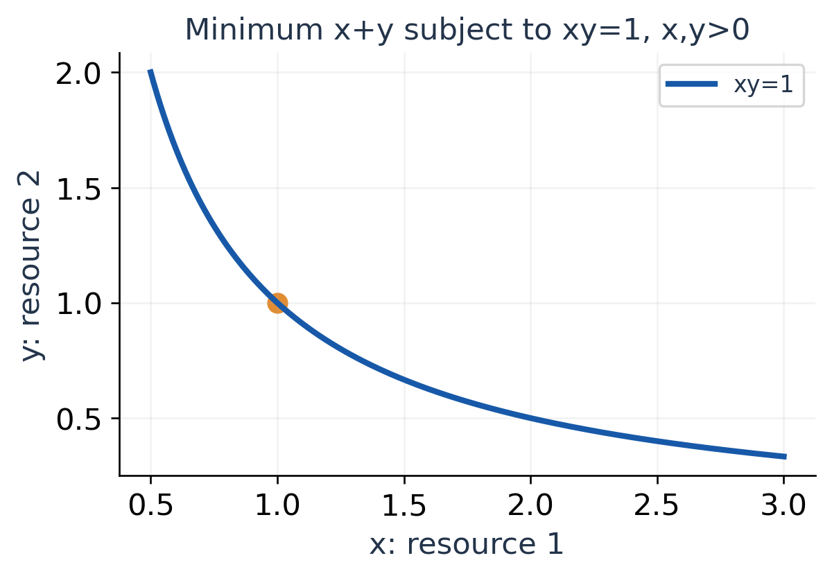
53. Solved Mixed Revision
Worked Example 1.91: Taylor and Error Estimate
Approximate ln(1+x+y) to second degree at the origin. Set s=x+y. The one-variable expansion ln(1+s)=s−s²/2+O(s³) gives:
T₂ = x+y−½(x²+2xy+y²)
For x=0.02, y=−0.01, s=0.01:
T₂ = 0.01−0.01²/2 = 0.00995
The exact value ln 1.01≈0.00995033. The domain condition 1+x+y>0 is satisfied.
Why the Mixed Term Appears
Although the function depends only on the sum, squaring that sum produces 2xy. Missing this term would change the second-order approximation.
The local power series is valid when |s|<1. A finite second-order Taylor approximation can also be discussed with an appropriate local remainder statement.
Worked Example 1.92: Logarithmic Euler Combinations
For u=ln(x+y) on x+y>0, first partials both equal 1/(x+y), so:
xuₓ+yuᵧ = 1
All three distinct second partials equal −1/(x+y)². Consequently:
x²uₓₓ+2xyuₓᵧ+y²uᵧᵧ = −1
The logarithm itself is not homogeneous of degree 1. Its inner expression is homogeneous, and the chain rule or direct partials give the stated constant combinations.
Worked Example 1.93: Combine Jacobian Properties
Let u=x+y, v=x−y and then p=u²+v², q=uv. Compute ∂(p,q)/∂(x,y).
The inner determinant is −2. The outer determinant is:
∂(p,q)/∂(u,v) = (2u)(u)−(2v)(v)
Thus the product is −4(u²−v²). Since u²−v²=4xy:
∂(p,q)/∂(x,y) = −16xy
Direct Verification
The composite outputs are p=2(x²+y²) and q=x²−y². Their determinant is:
(4x)(−2y)−(4y)(2x) = −16xy
The two independent routes agree. The determinant vanishes along either coordinate axis, so local inverse formulas requiring a nonzero determinant cannot be invoked there.
Mixed-Problem Method
Identify which part is a derivative calculation, which part is a coordinate transformation and which part is an approximation. Write the corresponding assumptions before combining formulas.
Worked Example 1.94: Differentiable Without C¹
For r=√(x²+y²)>0 define:
f = r² sin(1/r)
and set f(0,0)=0. Its origin partials are zero, and:
|f|/r ≤ r → 0
Thus f is differentiable at the origin with zero derivative. Away from the origin:
fₓ = 2x sin(1/r)−(x/r)cos(1/r)
Along the positive x axis, this derivative contains −cos(1/x) and has no limit at zero. So the first partials are not continuous there.
Continuous partials are a sufficient condition for differentiability, not a necessary one.
54. Short Answers with Reasoning
Do Matching Axis Limits Prove a Limit?
No. The function xy/(x²+y²) gives zero on both axes but 1/2 on y=x. Even agreement on every straight line can miss a curved path.
Does Continuity Imply Differentiability?
No. Differentiability requires a valid linear approximation with a sufficiently small relative remainder. Continuity only requires the output change to approach zero.
Can a Function Have Both Partials but No Derivative Map?
Yes. The example xy/√(x²+y²), defined as zero at the origin, has both origin partials zero and is continuous there, yet its diagonal differentiability ratio is 1/2.
When May Mixed Partials Be Interchanged?
Continuous second partials in a suitable neighbourhood provide a standard sufficient condition. Existence of the two mixed values at a single point alone does not guarantee equality.
What Is Held Fixed in a New-Coordinate Partial?
The other independent new coordinates are fixed. The original coordinates can both change through the transformation, so the chain rule is necessary.
Does a Nonzero Jacobian Give a Global Inverse?
It gives a local smooth inverse under the usual hypotheses. Global one-to-one behaviour also depends on the whole domain and repeated outputs.
Does D=0 Mean No Extremum?
No. The Hessian test is inconclusive. The origin is a minimum for x⁴+y⁴ and a saddle for x⁴−y⁴, although both have zero Hessian there.
Is a Lagrange Candidate Automatically the Answer?
No. Check constraint regularity, all candidates, any additional boundaries and the distinction between local and global optimisation.
Is a Differential an Exact Finite Error?
Generally no. It is the first-order part of the change. Exactness holds for a truly affine function, while nonlinear terms can produce a remainder or spoil a nominal worst-case estimate.
What Should a Complete Solution Show?
State the domain, relevant assumptions, derivative or transformation formula, substitution steps, final value and interpretation. If an approximation is used, mark it clearly and identify the neglected terms when possible.
Revision Focus
Most lost marks come from incomplete logic: an unproved limit, missing chain branch, shifted Taylor coefficient error, determinant sign error or unexamined boundary.
Worked Example 1.95: Exponential of a Homogeneous Input
Let u=exp(x³+y³). The inner function v=x³+y³ has degree 3, so:
xuₓ+yuᵧ = 3veᵛ
Because u=eᵛ>0 and v=ln u, the same answer is:
3u ln u
The outer exponential is not itself homogeneous of degree 3; the chain-rule factor is essential.
55. Final Formula Sheet
| Topic | Key Relation |
|---|---|
| Differentiability | Δf = fₓh+fᵧk+o(√(h²+k²)) |
| Differential | df = fₓdx+fᵧdy |
| One-parameter chain rule | dz/dt = fₓx′+fᵧy′ |
| Explicit t dependence | dz/dt = fₓx′+fᵧy′+fₜ |
| Implicit z from F=0 | zₓ = −Fₓ/F_z, zᵧ = −Fᵧ/F_z |
| Euler, degree n | xfₓ+yfᵧ = nf |
| Euler second order | x²fₓₓ+2xyfₓᵧ+y²fᵧᵧ = n(n−1)f |
| Second-degree Taylor | f₀+h(fₓ)₀+k(fᵧ)₀+½[h²(fₓₓ)₀+2hk(fₓᵧ)₀+k²(fᵧᵧ)₀] |
| Jacobian determinant | J = uₓvᵧ−uᵧvₓ |
| Local inverse | J_inverse = 1/J when applicable |
| Two-variable Hessian | D = fₓₓfᵧᵧ−(fₓᵧ)² |
| One equality constraint | ∇f = λ∇g, g=c at regular points |
| Linearised error estimate | E_lin = |fₓ|εₓ+|fᵧ|εᵧ |
Taylor coefficients are evaluated at the base point. Inverse and implicit formulas require nonzero relevant denominators. Hessian classifications assume a stationary point and suitable smoothness.
Final Self-Check with Answers
1. Find fₓ for f=x²y+sin y.
Holding y fixed gives 2xy.
2. If f is homogeneous of degree 4, find xfₓ+yfᵧ.
4f, under Euler’s differentiability and scaling assumptions.
3. Find ∂(x+y,x−y)/∂(x,y).
The determinant is −2; its area magnitude is 2.
4. What does D<0 mean at a C² stationary point?
The Hessian is indefinite in two variables, so the point is a saddle.
5. What must accompany the Lagrange equations?
The original constraint and checks for regularity, boundaries and complete candidate comparison.
6. A model has f=x²y. What is df/f for positive x,y?
2dx/x+dy/y. Use magnitudes to estimate a worst-case first-order relative error.
Last-Minute Problem Route
- Limits: Domain → quick laws → paths or uniform bound.
- Derivatives: Dependencies → correct fixed variables → chain paths.
- Optimisation: Feasible domain → candidates → classification → global checks.
- Approximation: Base point → derivative coefficients → signed changes → error interpretation.
Study Resources
Revise these Calculus and Linear Algebra Unit 1 Notes with the worked examples, graphs, derivative methods, approximation techniques and final formula sheet.
- More Study Material: https://www.notesgallery.com
- University: https://aktu.ac.in


