


University: Dr. A.P.J. Abdul Kalam Technical University (AKTU)
Programme: B.Tech First Year, Semester I
Course Code: AAS103D
Stream: CSE
Unit: IV – Matrices
Matrix notation: [[a,b],[c,d]] denotes a matrix with rows (a,b) and (c,d). A vertical bar separates coefficient and augmented blocks. Superscript ᵀ denotes transpose, † denotes conjugate transpose, and a tuple followed by ᵀ represents a column vector.
Unit IV Introduction
Matrices organise coefficients, transformations and coupled calculations. Row operations solve systems and reveal rank. Eigenvectors identify directions that a transformation scales without changing their line.
This unit develops real and complex matrices, inversion, elimination, iterative solution and diagonalisation. Applications connect these methods to coding, graphics, electrical loops and data analysis.
Complete Syllabus Map
| Topic | PDF Pages |
|---|---|
| Matrix notation and operations | 2–5 |
| Complex matrix classes | 6–10 |
| Elementary transformations and rank | 11–15 |
| Inverse by elementary transformations | 16–19 |
| Linear systems and Gauss elimination | 20–26 |
| Gauss–Seidel iteration | 27–32 |
| Eigenvalues and eigenvectors | 33–38 |
| Similarity, diagonalisation and powers | 39–43 |
| Stability interpretation | 44–45 |
| CSE and engineering applications | 46–53 |
| Solved revision and formula sheet | 54–56 |
Central Idea
Check dimensions, preserve complete equations during row operations, verify the result and distinguish exact algebra from numerical approximation.
Essential Notation
| Symbol | Meaning |
|---|---|
| A=[aᵢⱼ] | Entry in row i, column j |
| I, 0 | Identity and zero matrices |
| Aᵀ | Transpose |
| A† | Conjugate transpose |
| rank(A) | Number of pivot directions |
| [A:b] | Augmented system matrix |
| λ, v | Eigenvalue and nonzero eigenvector |
| S, D | Eigenvector and diagonal matrices |
| r=b−Ax | Residual |
The imaginary unit is i, with i²=−1. Vectors are columns unless stated otherwise. Here A† means conjugate transpose, not pseudoinverse.
Working Habits
- Check dimensions before multiplying.
- Apply operations to the entire augmented row.
- Count pivots in echelon form.
- Check solutions in the original equations.
- Use new Gauss–Seidel components immediately.
- Pair eigenvector columns with their eigenvalues.
- Distinguish discrete and continuous stability.
Application examples are specified educational models. No measured recognition accuracy or trained-system performance is claimed.
1. Matrix Notation and Dimensions
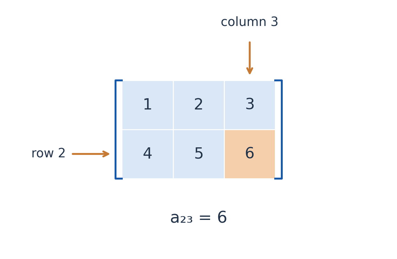
A matrix is a rectangular array. An m×n matrix has m rows and n columns. The entry aᵢⱼ lies in row i and column j; row index comes first.
A = [[1,2,3],[4,5,6]], A∈ℝ^(2×3).
Here a₂₃=6, a₁₂=2 and the second row is (4,5,6). The first column is (1,4)ᵀ. Dimensions describe shape, not just the total number of entries.

Worked Example 4.1 – Read an Entry
If B has rows (2,−1),(0,3),(4,5), it is 3×2 and b₃₂=5. The entry b₂₃ does not exist: B has no third column.
Two matrices are equal only when their dimensions and every corresponding entry agree. Equal row sums or determinants do not establish matrix equality.
Common Matrix Types
| Type | Feature |
|---|---|
| Row matrix | One row |
| Column matrix | One column |
| Square | Same row and column count |
| Diagonal | Off-diagonal entries zero |
| Scalar | All diagonal entries equal |
| Identity | Diagonal entries one |
| Zero | Every entry zero |
Worked Example 4.2 – Diagonal Versus Identity
D = [[2,0],[0,3]], I₂ = [[1,0],[0,1]].
D is diagonal but not scalar. The matrix 2I₂ is scalar and diagonal but is not identity. Both D and I₂ are square.
An upper triangular matrix has zeros below the main diagonal; a lower triangular matrix has zeros above it. Diagonal entries may themselves be zero.
Scope
Rectangular matrices have rank and can participate in compatible products. Ordinary determinant, inverse and eigenvalue problems in this unit concern square matrices.
2. Addition and Scalar Multiplication
Add equally sized matrices entry by entry. A scalar multiplies every entry, including negative and zero entries.
Worked Example 4.3 – Combine Two Matrices
A = [[1,−2],[3,0]], B = [[2,1],[−1,4]].
A+B = [[3,−1],[2,4]].
2A−B = [[0,−5],[7,−4]].
The upper-right entry of 2A−B is 2(−2)−1=−5. The lower-left is 2(3)−(−1)=7. Parentheses help preserve signs.
Worked Example 4.4 – Solve for a Matrix
If 2X+A=B, then X=(B−A)/2:
X = (1/2)[[1,3],[−4,4]].
This is division by a scalar, not inversion of a matrix.
Entrywise Rules and Checks
Addition is associative and commutative. Scalar multiplication distributes over sums. A zero matrix must have the appropriate shape for the equation in which it appears.
Worked Example 4.5 – An Incompatible Sum
A 2×3 matrix cannot be added to a 3×2 matrix. Both contain six entries, but their positions do not match. Equal entry count is not equal shape.
Worked Example 4.6 – Find Unknown Entries
[[x+1,2],[3,y−1]] = [[4,2],[3,5]].
Comparing entries gives x+1=4 and y−1=5, so x=3,y=6. The other corresponding entries already agree.

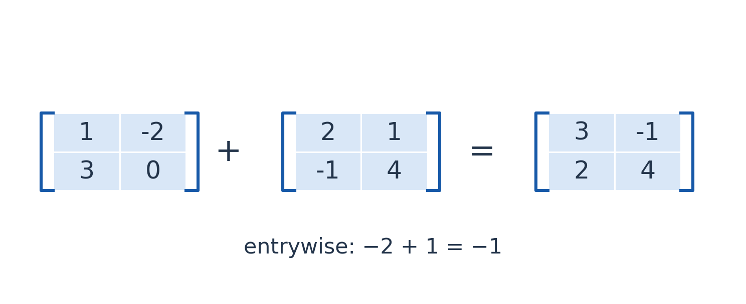
Equally sized measurement grids or image channels can be combined entrywise. This operation differs from matrix multiplication, which combines each output row–column pair by a dot product.
Check
First confirm equal dimensions. Then work position by position and retain parentheses around subtracted negative entries.
3. Matrix Multiplication
If A is m×n and B is n×p, AB exists and has dimensions m×p. The inner dimensions match; the output keeps the outer dimensions.
(AB)ᵢⱼ = Σ[k=1 to n] aᵢₖbₖⱼ.
Worked Example 4.7 – Multiply Two Matrices
A = [[1,2],[0,1]], B = [[2,0],[3,1]].
AB = [[8,2],[3,1]].
The upper-left entry is 1×2+2×3=8; the lower-right is 0×0+1×1=1. Every output entry uses a complete row and column.


Order Generally Matters
For the same matrices:
BA = [[2,4],[3,7]].
Thus AB≠BA. Associativity and distributivity hold when dimensions permit; commutativity does not hold in general.
Worked Example 4.8 – A Rectangular Product
C = [[1,0,2],[−1,3,1]], v = (2,1,−1)ᵀ.
Cv = (0,0)ᵀ.
The two dot products are 2−2=0 and −2+3−1=0. A nonzero input can map to zero when a direction is lost.
Zero Products and Cancellation
AB=0 need not imply either factor is zero. Nor may a matrix be cancelled from an equation without an appropriate invertibility or injectivity condition.
The identity satisfies AI=IA=A with matching sizes. The transpose reverses product order:
(AB)ᵀ = BᵀAᵀ.
Product Check
Write the dimensions before calculating. A numerical-looking expression is not a matrix product unless every required inner dimension matches.
4. Matrices as Transformations

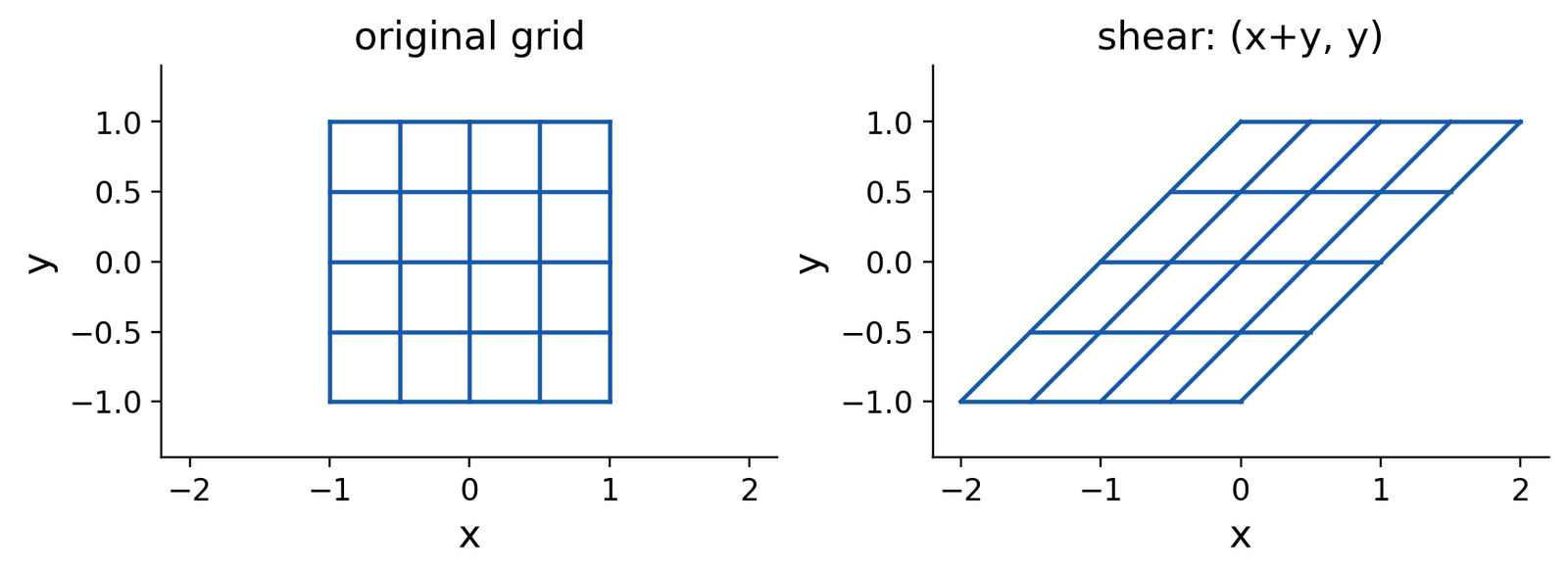
A matrix A maps a column x to Ax. Knowing the images of the coordinate unit vectors determines the image of every linear combination.
Worked Example 4.9 – Stretch the Plane
For S=diag(2,1), the point (1,1)ᵀ maps to (2,1)ᵀ. Horizontal distances double while vertical coordinates stay fixed.
Worked Example 4.10 – A Shear
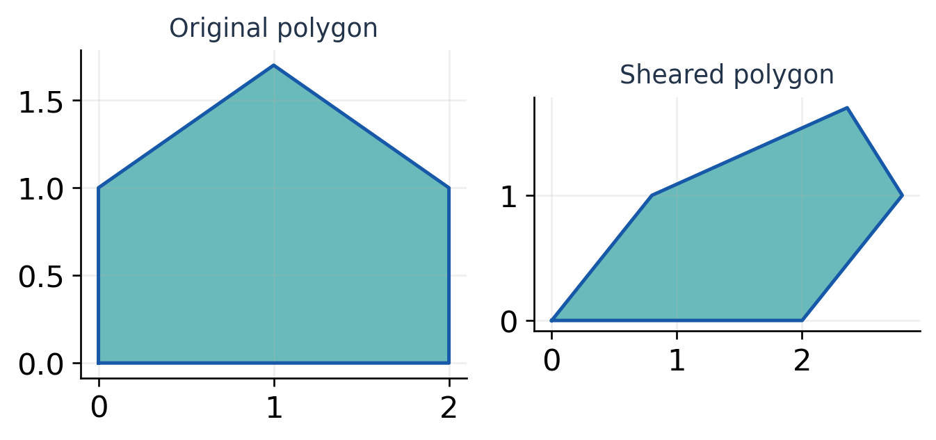
For H with rows (1,1),(0,1), the output is (x+y,y). Points shift horizontally by their y-coordinate. Horizontal lines retain their height, but lengths and angles generally change.
Composition and Geometry
For a 90° anticlockwise rotation:
R = [[0,−1],[1,0]].
With p=(1,1)ᵀ:
RSp = (−1,2)ᵀ, SRp = (−2,1)ᵀ.
The rightmost matrix acts first for column vectors.
A linear transformation fixes the origin and preserves sums and scalar multiples. A nonzero translation is therefore not represented by an ordinary 2×2 linear map alone. Homogeneous coordinates later provide a larger representation.
For 2×2 matrices, |det A| gives the area scale. Determinant zero indicates collapse into a line or point; a nonzero determinant means the transformation can be inverted.
Geometric Check
Transform both unit vectors and one test combination. If the combination does not match the proposed output, the columns or the composition order may be wrong.
A Shear’s Area Check
The unit square becomes a parallelogram with horizontal base one and vertical height one. Its area remains one, matching determinant one. The sloping side is longer than before, showing concretely why preserved area does not imply preserved lengths.

5. Transpose and Conjugate Transpose
Transpose exchanges rows and columns. Complex conjugation replaces i by −i. Conjugate transpose combines them:
A† = (conjugate of A)ᵀ.
Worked Example 4.11 – Keep the Operations Separate
A = [[1+i,2],[3i,4−i]].
Aᵀ = [[1+i,3i],[2,4−i]].
A† = [[1−i,−3i],[2,4+i]].
For a real matrix, A†=Aᵀ. With complex entries, transpose alone omits conjugation and usually produces a different result.
Useful Rules
(AB)† = B†A†.
(A†)† = A.
Worked Example 4.12 – A Rectangular Adjoint
For a 2×3 complex matrix, the adjoint is 3×2:
C = [[1,i,2],[0,1−i,3i]].
C† = [[1,0],[−i,1+i],[2,−3i]].
The first row becomes the first column after conjugation. Dimension reversal is a quick check that a transpose was actually performed.
Complex Inner Products
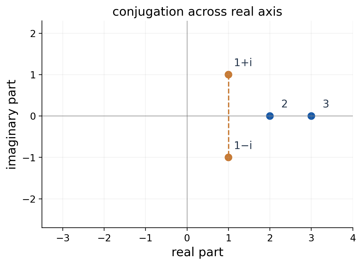
For complex columns, use u†v. The squared norm is v†v and is real and nonnegative.
Worked Example 4.13 – Complex Norm
For v=(1,i)ᵀ:
v†v = (1,−i)(1,i)ᵀ = 2.
By contrast, vᵀv=1+i²=0. That bilinear product is not the squared norm of the nonzero vector.
Worked Example 4.14 – Orthogonal Vectors
For u=(1,i)ᵀ and v=(i,1)ᵀ:
u†v = i−i = 0.
Without conjugation, uᵀv=2i.
A scalar also conjugates under the adjoint:
(cA)† = c̄A†.
Thus (iA)†=−iA†. The minus sign is essential in relating Hermitian and skew-Hermitian matrices.
Conjugation Check
Real entries stay fixed; imaginary parts change sign. If doing both operations mentally is difficult, first write the conjugated matrix and then transpose it.
Entrywise Adjoint Identity
For A=[aᵢⱼ], the adjoint’s entry in row i, column j is the conjugate of aⱼᵢ. Taking an adjoint twice restores both positions and conjugations.
For a real matrix, the conjugation step does nothing. This explains why real symmetric and orthogonal definitions can use transpose, while complex definitions need the adjoint.
6. Hermitian Matrices
A square complex matrix is Hermitian when:
H† = H.
Its diagonal entries are real, and opposite off-diagonal entries are conjugates. Real Hermitian matrices are exactly real symmetric matrices.
Worked Example 4.15 – Verify the Definition
H = [[2,1+i],[1−i,3]].
Conjugating and transposing returns H. Both diagonal entries are real and h₂₁=conjugate(h₁₂).
Worked Example 4.16 – Determine Entries
If H has rows (a,2+3i),(b,4), Hermitian symmetry requires a real and b=2−3i. It does not otherwise determine a.

Real Eigenvalues and Quadratic Values
Hermitian matrices have real eigenvalues and an orthonormal eigenvector basis over the complex numbers. Distinct-eigenvalue eigenvectors are orthogonal under u†v.
For every vector v, v†Hv is real, but it need not be positive.
Worked Example 4.17 – Not Always Positive
For H=diag(1,−2) and v=(0,1)ᵀ, v†Hv=−2. Hermitian does not mean positive definite.
Worked Example 4.18 – Check a Quadratic Value
For the displayed H and v=(1,i)ᵀ:
Hv = (1+i,1+2i)ᵀ.
v†Hv = (1+i)−i(1+2i) = 3.
The imaginary terms cancel, providing a useful check on adjoint signs.
The sum of same-size Hermitian matrices and any real scalar multiple remain Hermitian. A general complex scalar multiple need not.
Full Test
Real diagonal entries are necessary, not sufficient. Check the complete equality H†=H, including every off-diagonal pair.
7. Skew-Hermitian Matrices
A square complex matrix is skew-Hermitian if:
K† = −K.
Diagonal entries are purely imaginary or zero. Off-diagonal entries satisfy kⱼᵢ=−conjugate(kᵢⱼ).
Worked Example 4.19 – Verify All Signs
K = [[i,2+i],[−2+i,−2i]].
K† = [[−i,−2−i],[2−i,2i]] = −K.
The diagonal condition concerns real parts. The off-diagonal condition requires both conjugation and negation.


Connections to Hermitian Matrices
If H is Hermitian, iH is skew-Hermitian:
(iH)† = −iH† = −iH.
Conversely, iK is Hermitian when K is skew-Hermitian.
Worked Example 4.20 – Construct One
H = [[2,i],[−i,2]], iH = [[2i,−1],[1,2i]].
A skew-Hermitian matrix can have real off-diagonal entries, as ±1 show here. Its eigenvalues are purely imaginary or zero, not necessarily every entry.
Worked Example 4.21 – Quadratic Value
For K=iH:
v†Kv = i(v†Hv).
The bracketed scalar is real, so the result is purely imaginary.
In the real special case, Kᵀ=−K and all diagonal entries are zero. This is the familiar skew-symmetric condition.
Definition Check
“Skew” changes the adjoint relation by a minus sign. It does not mean ordinary transpose alone unless all entries are real.
Worked Example 4.22 – Imaginary Diagonal
K = [[i,0],[0,−i]].
Its adjoint is −K, so it is skew-Hermitian. It is also unitary because each diagonal entry has modulus one. Thus the classes can overlap without being identical. Their shared eigenvalues must lie on both the imaginary axis and the unit circle, namely i and −i.
8. Unitary Matrices
A square complex matrix is unitary when:
U†U = I.
It then also satisfies UU†=I and U⁻¹=U†. Its columns have unit complex norm and zero mutual inner products.
Worked Example 4.23 – Verify a Unitary Matrix
U = (1/√2)[[1,i],[i,1]].
U† = (1/√2)[[1,−i],[−i,1]].
The unscaled product has diagonal entries 2 and off-diagonal entries zero. The factor 1/2 therefore gives I.

Norm Preservation
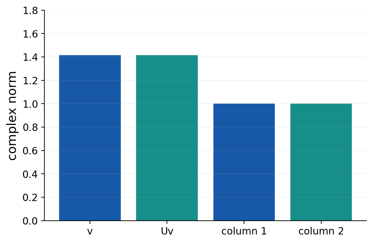
|Uv|² = v†U†Uv = v†v = |v|².
Worked Example 4.24 – Transform a Complex Vector
For v=(1,i)ᵀ:
Uv = (0,√2 i)ᵀ.
Both vectors have norm √2. A unitary transformation can change components while preserving inner products and total norm.
If Uv=λv and v≠0, norm preservation gives |λ|=1. The eigenvalues lie on the complex unit circle. Here they are (1±i)/√2.
A real unitary matrix is orthogonal: QᵀQ=I. Rotations preserve lengths and angles; a general shear does not.
Necessary Is Not Sufficient
Unitarity implies |det U|=1. But a matrix such as diag(2,1/2) also has determinant one and is not unitary, since it changes coordinate lengths.
Inverse Shortcut
Use U⁻¹=U† only after establishing unitarity. Complex entries or a determinant of modulus one do not establish it alone.


9. Comparing Complex Matrix Classes
| Class | Definition | Eigenvalue Location |
|---|---|---|
| Hermitian | H†=H | Real axis |
| Skew-Hermitian | K†=−K | Imaginary axis |
| Unitary | U†U=I | Unit circle |
These conditions can overlap, but they are not interchangeable.
Worked Example 4.25 – Hermitian but Not Unitary
The matrix 2I is Hermitian, yet (2I)†(2I)=4I. It does not preserve norms.
Worked Example 4.26 – Both Conditions
The diagonal matrix diag(1,−1) is Hermitian and unitary. A Hermitian unitary matrix satisfies H²=I, so its eigenvalues are ±1.
Uniqueness of the Decomposition
If a matrix is both Hermitian and skew-Hermitian, its adjoint equals both itself and its negative. Therefore it must be zero.
If A=H₁+K₁=H₂+K₂, the difference H₁−H₂ equals K₂−K₁. That difference belongs to both classes, so both differences vanish. The Hermitian-plus-skew-Hermitian decomposition is unique.
Decomposition of a Complex Matrix
Every square complex matrix splits into Hermitian and skew-Hermitian parts:
A = H+K, H = (A+A†)/2, K = (A−A†)/2.
Worked Example 4.27 – Find Both Parts
A = [[i,2],[0,1]].
H = [[0,1],[1,1]], K = [[i,1],[−1,0]].
The sum returns A, and adjoints verify H†=H, K†=−K. The alternative A=H+iG uses Hermitian G=(A−A†)/(2i).
The product A†A is always Hermitian and has nonnegative quadratic form:
v†A†Av = |Av|² ≥ 0.
It is not generally identity. Nonnegative quadratic form and unitarity are different conditions.
Classification
Compute the adjoint once, then test each defining equality separately. Appearance and diagonal entries alone are insufficient.
Worked Example 4.28 – Decomposition Check
For the stated A, H+K gives [[i,2],[0,1]], exactly A. Meanwhile H−K gives [[−i,0],[2,1]], exactly A†.
H+K = A, H−K = A†.
These two checks verify both parts without separately repeating every adjoint entry calculation.
10. Elementary Row Transformations
The elementary row operations are a row interchange, multiplication of a row by a nonzero scalar, and addition of a multiple of one row to another.
Rᵢ↔Rⱼ, Rᵢ←cRᵢ, c≠0.
Rᵢ←Rᵢ+cRⱼ, i≠j.
They are reversible. On an augmented system, they preserve the solution set only when the entire row, including its constant, is changed.
Worked Example 4.29 – Eliminate an Entry
[[1,2,3],[2,5,8]] → [[1,2,3],[0,1,2]] under R₂←R₂−2R₁.
Every entry in row 2 changes. The operation does not affect just the leading coefficient.


Elementary Matrices
An elementary matrix comes from applying one row operation to identity. Left multiplication performs that operation on another matrix.
Worked Example 4.30 – A Row-Addition Matrix
E = [[1,0],[−2,1]], E⁻¹ = [[1,0],[2,1]].
EA leaves row 1 fixed and replaces row 2 by row 2−2row 1. The inverse adds twice row 1 back.
Left multiplication produces row operations; right multiplication by suitable elementary matrices produces column operations. Both preserve rank when invertible, but column operations can change variable coordinates.
Do not freely operate on coefficient columns of an augmented system and then read the old variable names without tracking the change.
Why Zero Scaling Is Excluded
Multiplication of a row by zero erases its information and cannot generally be reversed. It is therefore not an elementary operation.
Operation Log
Write the operation before displaying the new matrix. Keep unchanged rows copied accurately so that each step can be checked independently.
11. Echelon Form and Pivots
In row echelon form, zero rows are at the bottom, each leading nonzero entry lies to the right of the one above, and entries below each leading position vanish.
Leading entries are pivots. They need not equal one until a normalised form is requested.
Worked Example 4.31 – Echelon to Reduced Echelon
E = [[1,2,0],[0,3,6],[0,0,0]].
Scale row 2 by 1/3 and subtract twice that row from row 1:
rref(E) = [[1,0,−4],[0,1,2],[0,0,0]].
Each pivot is now one and is the only nonzero entry in its column.

Systematic Reduction
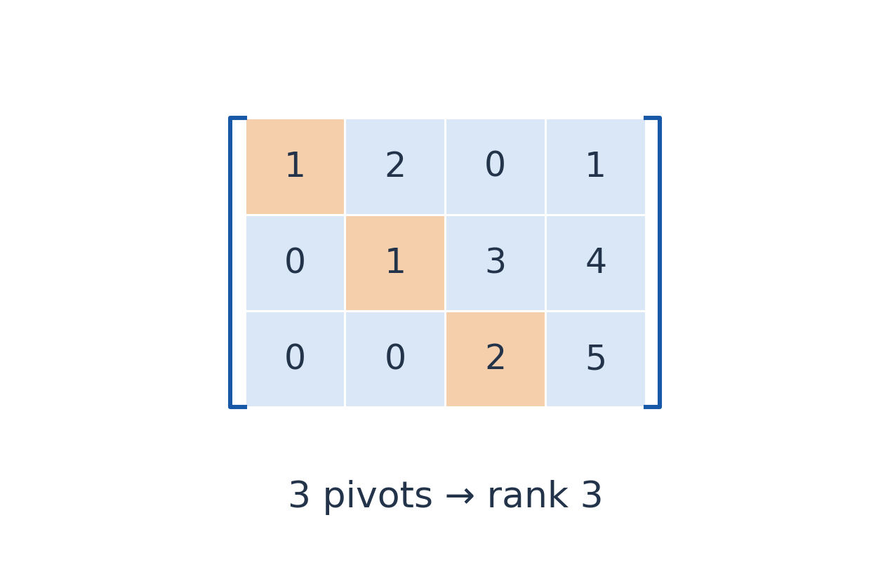
- Step 1: Find a nonzero candidate in the current column.
- Step 2: Swap a suitable row into the pivot position if needed.
- Step 3: Eliminate entries below that pivot.
- Step 4: Move to the next row and a later column.
- Step 5: Continue until no further pivots remain.
Worked Example 4.32 – A Skipped First Column
A = [[0,1,2],[0,2,4]].
R₂←R₂−2R₁ leaves one nonzero row. Its pivot is in column 2, so rank(A)=1 despite the zero first column.
Counting original nonzero diagonal entries does not generally give rank. Rectangular matrices and skipped pivot columns make that shortcut especially unreliable.
Echelon forms can vary with row choices. Reduced row echelon form is unique over the stated field, and the number of pivots is invariant.
Zero Candidate
Look below for a row swap or move to a later column. Never divide by zero, and do not conclude that the whole matrix has rank zero from one zero candidate.
12. Rank by Echelon Form
Rank equals the number of pivots in an echelon form, or the number of nonzero rows after valid forward reduction.
Worked Example 4.33 – Rank Two
A = [[1,2,3],[2,4,6],[1,1,1]].
Use R₂−2R₁ and R₃−R₁, then swap rows 2 and 3:
E = [[1,2,3],[0,−1,−2],[0,0,0]].
Two pivots remain, so rank(A)=2. The second original row was dependent on the first, but the third supplied another direction.

Rectangular Full Rank
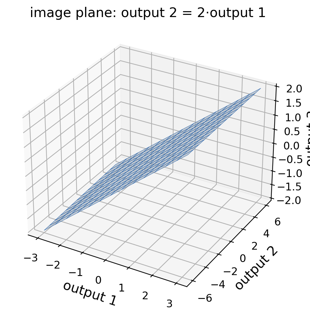
For m×n matrices, rank≤min(m,n). Full row rank means rank=m; full column rank means rank=n.
Worked Example 4.34 – A 2×3 Matrix
B = [[1,0,2],[0,1,−1]].
It has two pivots: full row rank, but not full column rank because it has three columns.
Worked Example 4.35 – Zero Rank
Every zero matrix has rank zero. Every nonzero matrix has rank at least one, regardless of shape.
For the original A, pivot columns 1 and 2 are independent original columns. Its third column obeys:
c₃ = −c₁+2c₂.
Check using the original columns:
−(1,2,1)+2(2,4,1) = (3,6,1).
Reduced columns should not be substituted when describing the original data directions.
Determinant Limit
For square A, determinant zero says rank is below full size. It does not identify the exact smaller rank; use pivots or suitable nonzero minors.
Worked Example 4.36 – A Lost Input Direction
For the rectangular B, choose z=t in Bx=0. Then x=−2t and y=t:
B(−2,1,1)ᵀ = (0,0)ᵀ.
The nonzero vector is a direction lost by the map. Two pivots among three inputs leave exactly one free parameter in this homogeneous system.

13. Rank with a Parameter
Elimination identifies exceptional parameter values at which a pivot disappears. Before dividing by a parameter expression, separate its zero case.
Worked Example 4.37 – A Final Pivot Changes
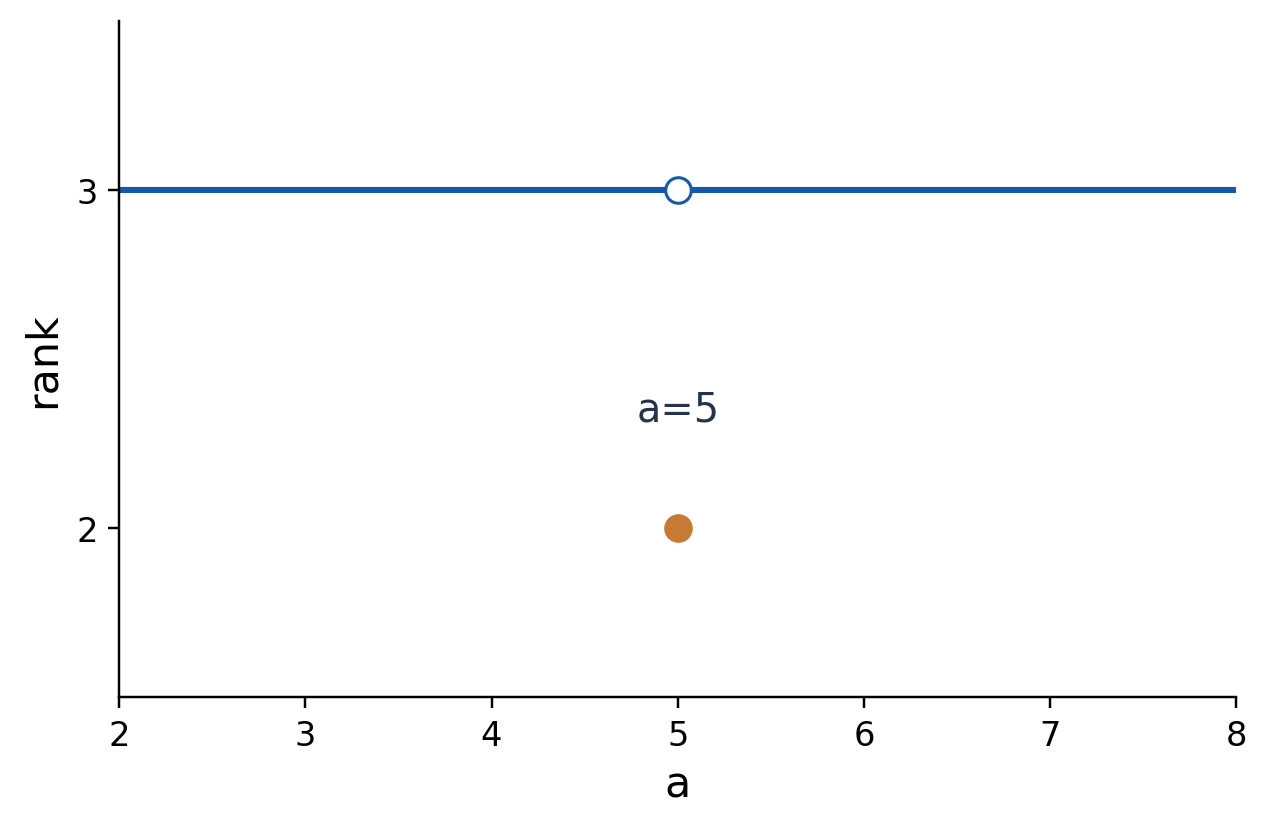
A = [[1,1,1],[1,2,3],[1,3,a]].
Subtract row 1 from rows 2 and 3, then subtract twice the new row 2 from row 3:
E = [[1,1,1],[0,1,2],[0,0,a−5]].
For a≠5, rank is 3. At a=5, the last row vanishes but two earlier pivots survive, so rank is 2.

Worked Example 4.38 – A Two-Value Exception
B = [[1,t],[t,1]], det B = 1−t².
For t≠±1, rank is 2. At t=1, rows coincide; at t=−1, one is the negative of the other. Each exception has rank 1.
The rank never becomes zero because the diagonal entries remain one.
For the 3×3 example, row additions preserve determinant and the triangular form gives det A=a−5. The nonzero leading 2×2 pivot block shows why the rank cannot fall below two at a=5.
An Unsafe Step
Dividing the last row by a−5 and continuing as if it always equals one discards the case a=5. The answer must state both alternatives.
Case Rule
One vanished pivot does not erase earlier pivots. Return to the unscaled form and count all surviving nonzero rows in the exceptional case.
Worked Example 4.39 – Inspect Both Exceptions
At t=1 and t=−1 the matrices are:
B₊ = [[1,1],[1,1]], B₋ = [[1,−1],[−1,1]].
Each has one nonzero row after elimination. Their first entries stay one, so neither can have rank zero. Checking the exceptional matrices directly confirms that no extra case has been missed.
14. Rank Properties
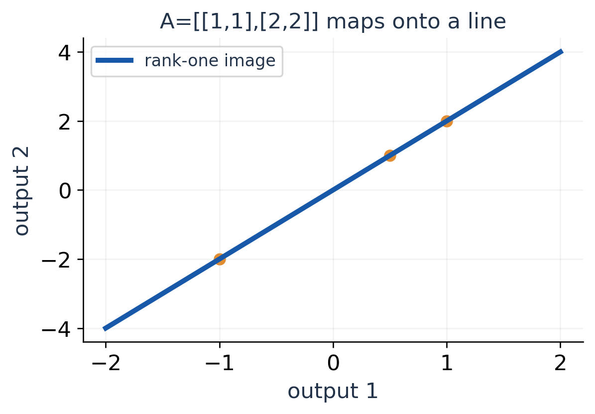
Invertible row and column transformations preserve rank. Transpose preserves rank, so row rank equals column rank.
rank(A) = rank(Aᵀ).
rank(AB) ≤ min(rank A,rank B).
Worked Example 4.40 – A Rank-One Product
A = [[1,2],[2,4]], B = [[1,0],[0,3]].
AB = [[1,6],[2,12]].
The product has rank one. Here B is invertible, so multiplying by it preserves A’s rank exactly.
Rank and Invertibility
For n×n matrices, full rank, nonzero determinant, existence of an inverse and unique solvability of Ax=b for every b are equivalent.
Worked Example 4.41 – A Projection
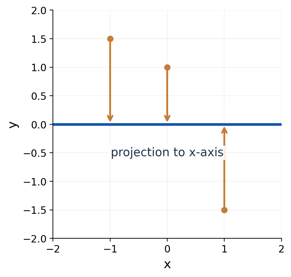
P = [[1,0],[0,0]].
Its rank is one and its determinant is zero. It maps (x,y) to (x,0), losing the y-coordinate. Different inputs therefore share the same output.
Worked Example 4.42 – Rank Is Not Trace
The matrix diag(2,3) has rank 2 but trace 5. The equality for some projections is not a general rule.
Rank(A+B)≤rank(A)+rank(B), but equality need not hold. If B=−A, the sum has rank zero even when both inputs have positive rank.

Interpretation
Rank counts independent surviving directions. Trace, determinant and the count of nonzero entries cannot replace a pivot calculation.
Why Invertible Multiplication Preserves Rank
The product inequality gives rank(AB)≤rank(A). If B is invertible, write A=(AB)B⁻¹ and apply the inequality again to obtain the reverse inequality. Therefore the ranks are equal. Reversible coordinate changes cannot create or destroy independent directions.
15. What an Inverse Means
A square A has an inverse if:
AA⁻¹ = A⁻¹A = I.
The inverse reverses its linear transformation. It exists precisely for full-rank square matrices.
Worked Example 4.43 – Verify a Proposed Inverse
A = [[2,1],[1,1]], B = [[1,−1],[−1,2]].
Both AB and BA equal I₂, so B=A⁻¹. Taking reciprocals of individual entries would not produce this inverse.
Worked Example 4.44 – Diagonal Case
For D=diag(2,3), the inverse is diag(1/2,1/3). The diagonal shortcut works because there is no off-diagonal coupling and neither diagonal value is zero.
Worked Example 4.45 – Two Right-Hand Sides
Using the same A and its inverse, solve AX=B for:
B = [[5,3],[3,2]].
X = A⁻¹B = [[2,1],[1,1]].
Each column of X solves the system for the corresponding column of B. Inverse multiplication handles both right-hand sides together while preserving their order.
Inverse Rules and Uses
(AB)⁻¹ = B⁻¹A⁻¹, (A⁻¹)⁻¹ = A.
(Aᵀ)⁻¹ = (A⁻¹)ᵀ.
The product rule requires both square factors invertible and reverses their order. Undo the last action first.
Worked Example 4.46 – Solve Using the Inverse
For the displayed A and b=(5,3)ᵀ:
A⁻¹b = (2,1)ᵀ.
Substitution gives 2(2)+1=5 and 2+1=3.
An inverse explains solvability, but numerical systems are normally solved directly rather than forming an explicit inverse without need.
To calculate an inverse by elementary transformations, start from [A:I]. Reduce the left block to I, applying every operation across both blocks. The right block then becomes A⁻¹.
Verification
A correct determinant does not verify every inverse entry. Multiply the proposed inverse with A and check the identity.
Verification by Columns
For the preceding X, A times column (2,1) gives (5,3), while A times (1,1) gives (3,2). Thus AX=B exactly.
The right-hand-side columns are independent problems with a shared coefficient matrix. This explains why an inverse contains information for every possible right-hand side, even though forming it explicitly is not always the best numerical procedure.
16. Inverse by Row Transformations
Worked Example 4.47 – A 2×2 Gauss–Jordan Inverse
Form [A:I] and swap rows:
[[2,1|1,0],[1,1|0,1]] → [[1,1|0,1],[2,1|1,0]] under R₁↔R₂.
Use R₂←R₂−2R₁ and then R₂←−R₂:
[[1,1|0,1],[0,1|−1,2]].
Finally R₁←R₁−R₂ gives:
[[1,0|1,−1],[0,1|−1,2]].
The right block is the inverse. The augmentation line separates roles, not operations.
What Each Inverse Column Solves
The first identity column asks for a vector u satisfying Au=e₁. The second asks for Av=e₂. The augmented identity therefore records several solves at once.
For this example, u=(1,−1)ᵀ and v=(−1,2)ᵀ. Placing them as columns reproduces the computed inverse. This interpretation also extends to larger square matrices.
Why the Method Works
Let E represent the product of elementary row-operation matrices. The augmented blocks become [EA:E]. When EA=I, E=A⁻¹, establishing the right block’s meaning.
Worked Example 4.48 – Multiply Back
[[2,1],[1,1]][[1,−1],[−1,2]] = [[1,0],[0,1]].
For example, the upper-right entry is −2+2=0. Checking all four entries confirms the result independently.
A convenient pivot can avoid fractions. A larger available pivot can also reduce rounding amplification in numerical calculations. Any row swap must move the identity-block entries as well.
Write each operation beside its resulting matrix. If several operations are performed, make clear whether they use old or already updated rows.
Full-Row Rule
Changing only A while leaving I fixed does not record the inverse operations. Apply every row transformation to the entire augmented matrix.
Worked Example 4.49 – Check Each Inverse Column
A(1,−1)ᵀ = (1,0)ᵀ, A(−1,2)ᵀ = (0,1)ᵀ.
The two equations check the entire inverse product column by column. This is often clearer than checking four output entries without explaining why identity appears. Reversing the column order would instead produce a permutation matrix, not identity.
17. A Complete 3×3 Inverse
Worked Example 4.50 – Forward Reduction
A = [[1,1,0],[0,1,1],[1,0,1]].
In [A:I], use R₃←R₃−R₁ and then R₃←R₃+R₂:
[[1,1,0|1,0,0],[0,1,1|0,1,0],[0,0,2|−1,1,1]].
Scale row 3 by 1/2:
[[1,1,0|1,0,0],[0,1,1|0,1,0],[0,0,1|−1/2,1/2,1/2]].
The left block is now upper triangular with unit pivots. Entries above the last pivot still require elimination.
Worked Example 4.51 – Solve for the Third Inverse Column
Set b=e₃. The equations become x+y=0, y+z=0, x+z=1. The first two give y=−x and z=x; the last gives x=1/2.
A⁻¹e₃ = (1/2,−1/2,1/2)ᵀ.
This is exactly column 3 of the inverse. It checks the signs in the most recent pivot row.
Backward Reduction
Use R₂←R₂−R₃ and then R₁←R₁−R₂. The result has left block I and:
A⁻¹ = (1/2)[[1,−1,1],[1,1,−1],[−1,1,1]].
To verify AA⁻¹, its first row adds rows 1 and 2 of A⁻¹, giving (1,0,0). Its second adds rows 2 and 3, giving (0,1,0). Its third adds rows 1 and 3, giving (0,0,1).
Worked Example 4.52 – Solve with the Inverse
A⁻¹(3,5,4)ᵀ = (1,2,3)ᵀ.
The original equations are x+y=3, y+z=5, x+z=4; all are satisfied.
The forward pivots 1,1,2 give determinant 2 because no row swaps occurred. This agrees with invertibility.
Backward Order
Use the current updated row 2 in the final operation. An older copy of that row would produce an incorrect right block.
Determinant and Trace Cross-Checks
Since det A=2, det(A⁻¹) must be 1/2. The displayed inverse satisfies this reciprocal rule. Its trace is 3/2 because all three diagonal entries are 1/2.
Trace of an inverse is not generally the reciprocal of trace. Here trace A=3, whose reciprocal is 1/3, different from 3/2. Only eigenvalue-wise reciprocation is the valid general rule.
18. Singular Matrices and Matrix Equations
A singular matrix cannot be reduced to identity by elementary row operations. A missing pivot remains, and no ordinary inverse exists.
Worked Example 4.53 – Detect Singularity
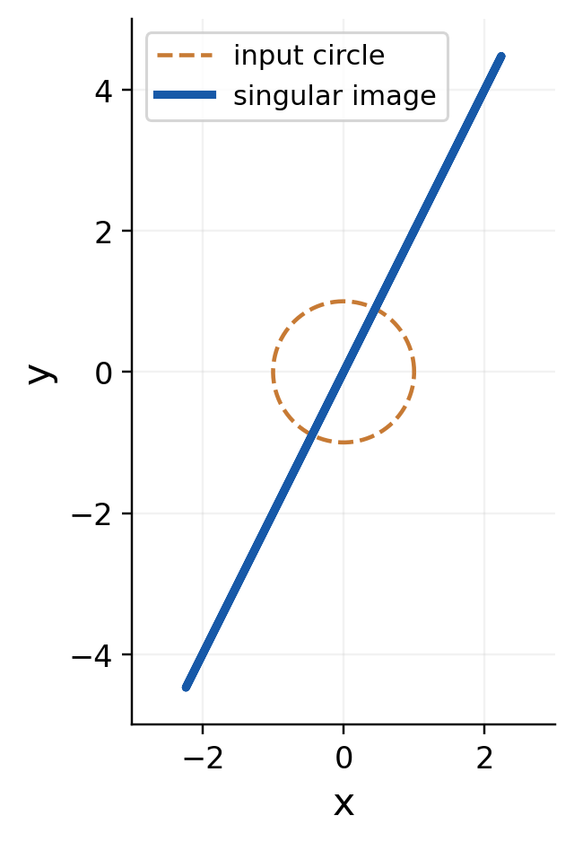
A = [[1,2],[2,4]].
R₂←R₂−2R₁ gives a zero coefficient row. Rank is one, determinant is zero and inversion fails.
Some systems Ax=b with this A are consistent with infinitely many solutions; others are inconsistent. Singularity alone does not choose between these cases.

Worked Example 4.54 – AX=B
For invertible A, left multiplication gives:
AX = B ⇒ X = A⁻¹B.
For XA=B, multiply on the right:
X = BA⁻¹.
These expressions generally differ because products do not commute.
Worked Example 4.55 – A Two-Sided Equation
If AXB=C and both A,B are invertible:
X = A⁻¹CB⁻¹.
The inverse factors are placed next to the factors they cancel. Moving them across C without a valid commutation relation changes the equation.
Check every product’s dimensions, then substitute the result into the original equation. A dimensionally impossible expression cannot be repaired by numerical manipulation.
Singular Warning
A failed exact pivot is not replaced by an invented small number. Investigate rank and consistency instead of pretending an inverse exists.
19. Linear Systems as Ax=b

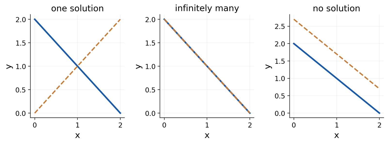
Each matrix row represents an equation, each column corresponds to a variable, and b contains the constants. Keep one variable order throughout.
Worked Example 4.56 – Build the Augmented Matrix
The equations x+y+z=6, 2x+3y+z=11, x−y+2z=5 give:
[A:b] = [[1,1,1|6],[2,3,1|11],[1,−1,2|5]].
A missing variable has coefficient zero; its column must remain in place.
Coefficient and Output Spaces
The input column contains variable values. Multiplying by A produces the three equation left sides, which must equal b.
For the candidate (1,2,3), the output is (6,11,5). A different b changes the target intersection even when A stays fixed. This is why consistency belongs to the augmented matrix, not to the coefficients alone.
Geometry and Verification
In two variables, nondegenerate equations describe lines. In three variables they describe planes, whose intersection can be a point, line, plane or empty set.
Worked Example 4.57 – Check a Candidate
For (x,y,z)=(1,2,3), the three original left sides are 6,11,5. The candidate solves the displayed system. Uniqueness still requires a rank or invertibility argument.
A homogeneous system has b=0 and always contains the zero solution. Nonzero solutions exist when fewer pivots than unknowns remain.
Matrix Translation
Fix the variable order before writing coefficients. A sign or column-order mistake changes the problem before elimination starts.
20. Gauss Elimination: Two Variables
Gauss elimination uses forward reduction to obtain a triangular system, then back substitution. Gauss–Jordan additionally eliminates above pivots, as used for inverses.
Worked Example 4.58 – Solve Two Equations
For 2x+y=5 and x−y=1, swap rows to use a first pivot of one:
[[1,−1|1],[2,1|5]] → [[1,−1|1],[0,3|3]] under R₂←R₂−2R₁.
The last equation gives y=1; the first gives x=2. Both satisfy the originals.


Elimination Versus Gauss–Jordan
Gauss elimination stops its forward phase once entries below pivots vanish, then uses substitution. Gauss–Jordan continues until every pivot column has zeros above as well.
Both are valid exact methods, but their stopping forms differ. An upper triangular coefficient matrix is enough for substitution; the identity left block is required when reading an inverse from [A:I].
Back Substitution in Order
Start at the last nonzero equation, which has the fewest remaining unknowns, and work upward.
Worked Example 4.59 – A Triangular System
2x+y−z=1, 3y+2z=12, 4z=12.
From the bottom, z=3. Then 3y+6=12 gives y=2. Finally 2x+2−3=1 gives x=1.
In the first example, the eliminated constant is 5−2(1)=3. Leaving it at 5 would fail to preserve the equation.
Retain exact fractions when convenient. Premature decimal rounding can create a misleading final residual even when the method is correct.
A complete presentation records row operations, triangular equations and back substitution, then checks the solution in the original system.
Forward Then Backward
Do not try to read all unknowns directly from an upper triangular matrix. Earlier rows still contain later variables and need substitution.
21. Gauss Elimination: Three Variables
Worked Example 4.60 – Forward Elimination
For x+y+z=6, 2x+3y+z=11, x−y+2z=5, use R₂−2R₁ and R₃−R₁:
[[1,1,1|6],[0,1,−1|−1],[0,−2,1|−1]].
Then R₃←R₃+2R₂ gives:
[[1,1,1|6],[0,1,−1|−1],[0,0,−1|−3]].
All three pivots are nonzero. The coefficient matrix has rank three and the solution is unique.


Back Substitution and Independent Checks
The last row gives z=3. The second gives y−3=−1, so y=2. The first gives x+2+3=6, so x=1.
(x,y,z) = (1,2,3).
Original-Equation Check
- First: 1+2+3=6.
- Second: 2+6+3=11.
- Third: 1−2+6=5.
Every residual is zero. Checking only the reduced equations might miss a copying error made during reduction.
Only row-addition operations occurred, so determinant was preserved. The triangular pivot product is −1, agreeing with full rank.
Use the updated row 2 in the final elimination. Substituting an old version of row 2 into R₃+2R₂ would be a different operation.
Rank Interpretation
If a final coefficient row vanishes, do not divide by zero. Read the augmented constant to distinguish compatibility and contradiction.
Worked Example 4.61 – Reject a Nearby Candidate
Try (1,2,2) in the original three equations. The left sides are (5,10,3), while b=(6,11,5).
r = b−A x̃ = (1,1,2)ᵀ.
The nonzero residual rejects this candidate. A solution must satisfy every equation, not merely resemble the expected integers or satisfy one selected row.
22. Pivoting and Row Swaps
A zero pivot candidate requires a search below it. A row swap may provide a nonzero pivot without changing the solution set.
Worked Example 4.62 – A Zero Initial Entry
The equations y+z=3, x+y=3, x+z=4 have a zero upper-left coefficient. Swapping the first two rows gives a usable pivot. Elimination yields:
(x,y,z) = (2,1,2).
The original zero candidate did not make the matrix singular.
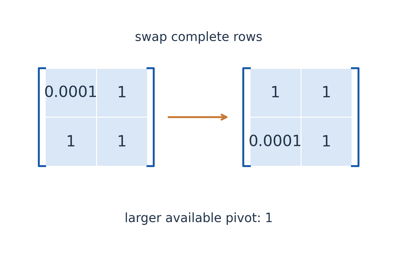
Partial pivoting selects the largest-magnitude remaining entry in the current column. This avoids unnecessary division by a tiny number and often improves numerical robustness.

Worked Example 4.63 – Compare Pivot Sizes
10^(−4)x+y=1, x+y=2.
Without swapping, the first elimination multiplier is 10,000. After swapping, it is 10^(−4). In exact arithmetic either route gives x=1/(1−10^(−4)), y=2−x.
Finite-precision subtraction is more exposed in the large-multiplier route. Pivoting helps, but cannot remove a problem’s inherent sensitivity or guarantee that every small residual means a small solution error.
A row swap reverses determinant sign. Row scaling multiplies it by the scale, while adding a multiple of another row preserves it. Include these changes if reconstructing a determinant from pivot products.
Pivot Rule
Never divide by zero. In parameter problems, split exceptional cases; in numerical problems, use a better available pivot instead of an avoidably tiny one.
Worked Example 4.64 – Exact Small-Pivot Solution
Solving the two displayed equations exactly gives:
x = 10000/9999, y = 9998/9999.
Their sum is two and the first equation also checks exactly. Rounded to four decimal places, they are about 1.0001 and 0.9999. A near-one answer is plausible, but the exact fractions expose the small difference that finite precision may hide.
23. Consistency by Rank
For n unknowns, a system is consistent exactly when rank(A)=rank([A:b]). If that common rank is n, the solution is unique. If it is r<n, free variables remain and infinitely many real or complex solutions exist.
Worked Example 4.65 – Contradictory Equations
For x+y=2 and 2x+2y=5:
[[1,1|2],[2,2|5]] → [[1,1|2],[0,0|1]].
The last row means 0=1. Coefficient rank is 1 and augmented rank is 2, so no solution exists.
Worked Example 4.66 – Compatible Dependence
If the second constant is 4 instead, the last row becomes all zeros. Both ranks are 1; the equations repeat the same restriction.
Read the Entire Augmented Row
A zero coefficient row with zero constant adds no restriction. A nonzero constant creates a contradiction.
Worked Example 4.67 – Infinite Family
For x+y=2, 2x+2y=4, set y=t:
(x,y) = (2−t,t), t∈ℝ.
Every parameter value solves both equations. A single guessed member would not describe the complete solution set.
Worked Example 4.68 – Unique Solution
For x+y=2, x−y=0, rank is 2 and x=y=1. No free variable remains.

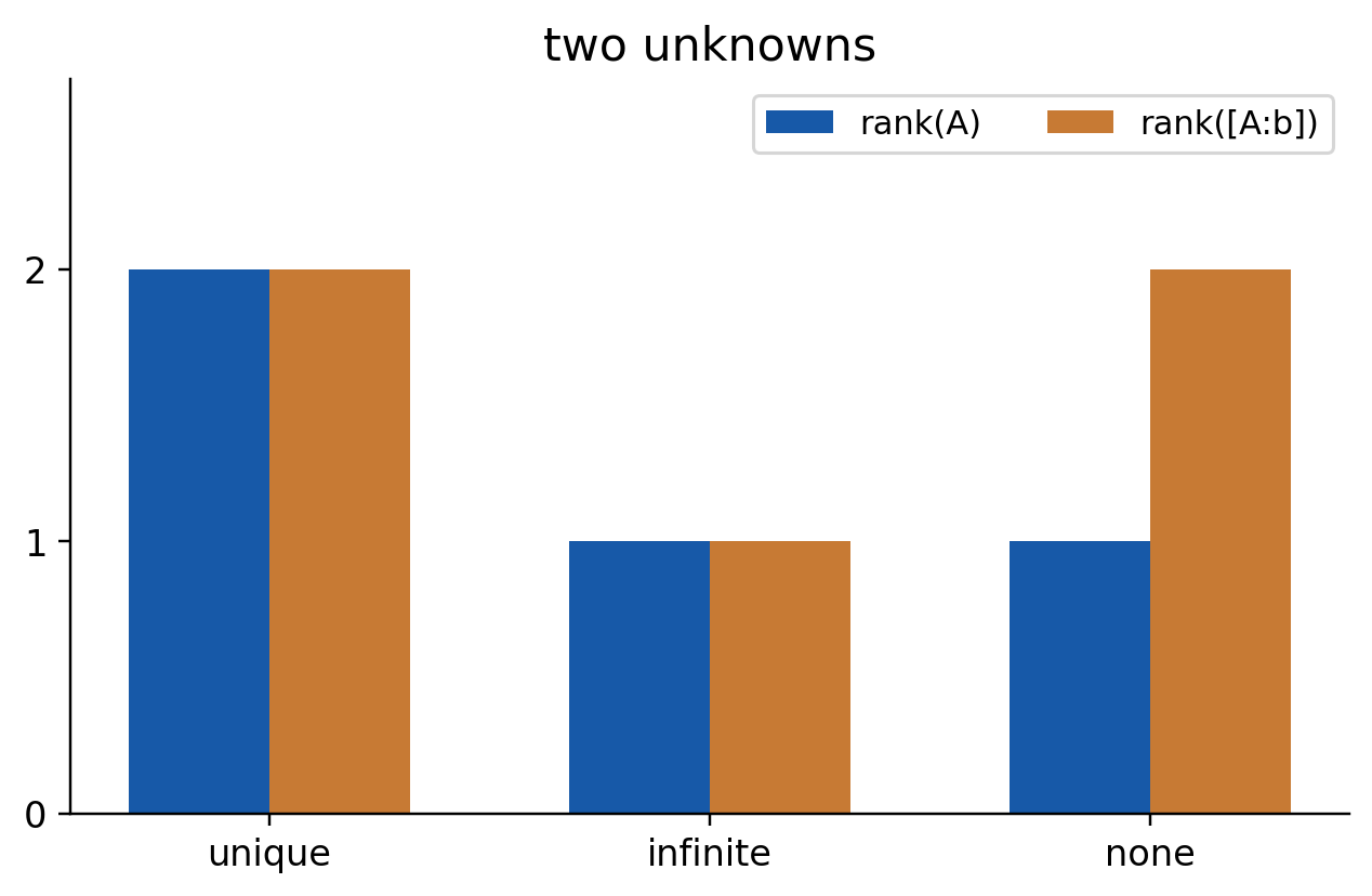
A homogeneous system is always consistent because its constants are all zero. It has nonzero solutions exactly when its rank is below the number of unknowns.
Singularity
Determinant zero says unique solvability fails for a square coefficient matrix. It does not alone distinguish infinitely many solutions from no solution.
Worked Example 4.69 – Compatibility with a Parameter
For x+y=2 and 2x+2y=a, elimination gives 0=a−4. Thus a=4 produces infinitely many solutions and every other a gives none.
| Parameter | Coefficient Rank | Augmented Rank |
|---|---|---|
| a=4 | 1 | 1 |
| a≠4 | 1 | 2 |
The coefficient matrix is unchanged; only the constant changes compatibility.


24. Free Variables and Solution Families
A consistent system with r pivots among n unknowns has n−r free variables. Parameterise nonpivot variables, then determine pivot variables from the equations.
Worked Example 4.70 – Two Equations in Three Unknowns
For x+y+z=3 and x−y+z=1, subtraction gives y=1 and then x+z=2. Set z=t:
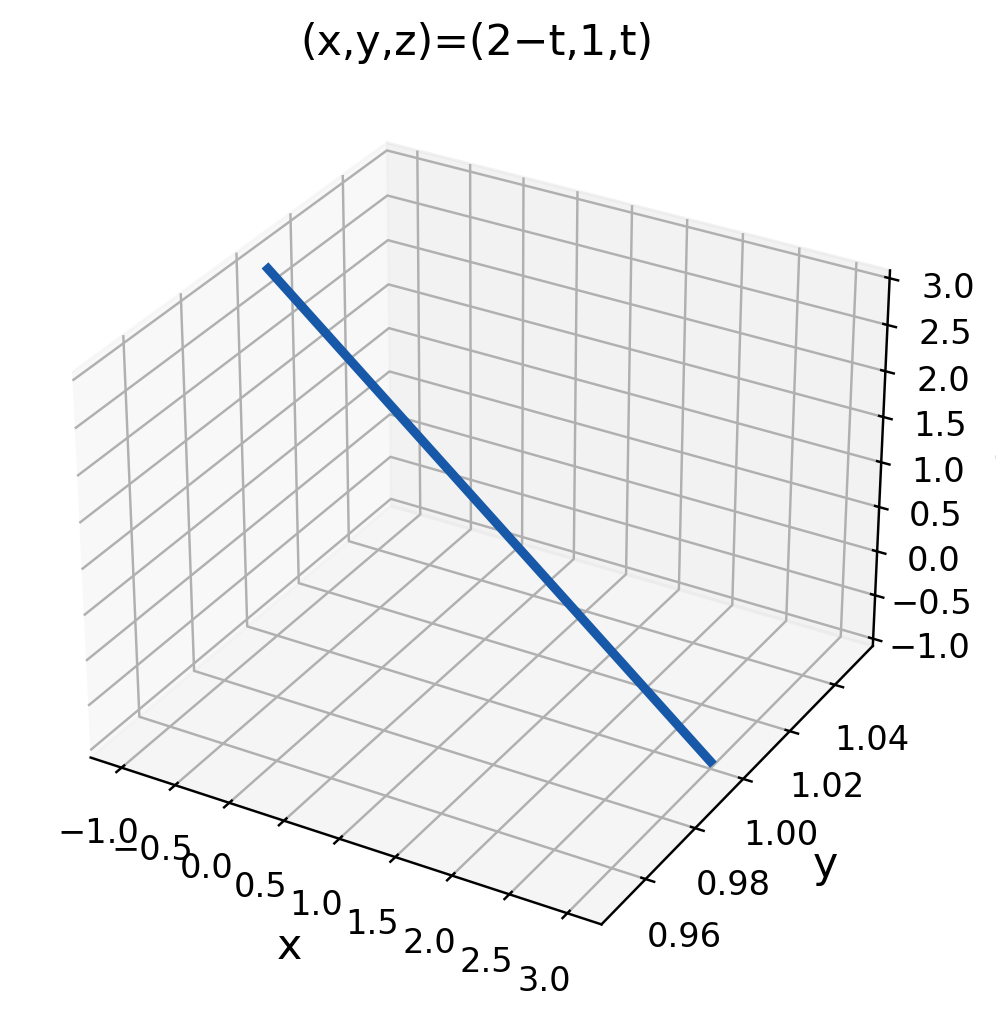
(x,y,z) = (2−t,1,t).
(x,y,z)ᵀ = (2,1,0)ᵀ+t(−1,0,1)ᵀ.
The fixed vector is one particular solution. The direction vector solves the corresponding homogeneous system.

Check the Complete Family
Substitute x=2−t,y=1,z=t. The two left sides simplify to 3 and 1 for every t, proving the entire family works.
Worked Example 4.71 – Two Free Parameters
For x+2y−z=0, choose y=s,z=t, giving:
(x,y,z) = s(−2,1,0)+t(1,0,1).
One pivot leaves two parameters. Setting both to zero gives the zero solution; other values give nonzero solutions.
Do not assign an extra independent parameter to a pivot variable after all free variables have been parameterised. The equations already determine it.
If the field is complex, parameters are complex rather than real. The formula is the same but its permitted parameter values differ.
Completeness
Count parameters and compare with n−rank(A). Then substitute the family into the original system rather than checking only one parameter choice.
A Different Parameter, Same Line
In the first family, choose x=s instead of z=t. Then y=1 and z=2−s, giving (s,1,2−s).
These describe the same line because s=2−t relates the parameters. A different-looking parameterisation need not be a different solution set. Check its equations and range before declaring two families inconsistent.
25. Residuals and Numerical Verification
For an approximate solution x̃, define:
r = b−A x̃.
It measures how far the equations fail to be satisfied. It is not the same as the unknown solution error x−x̃.
Worked Example 4.72 – Calculate a Residual
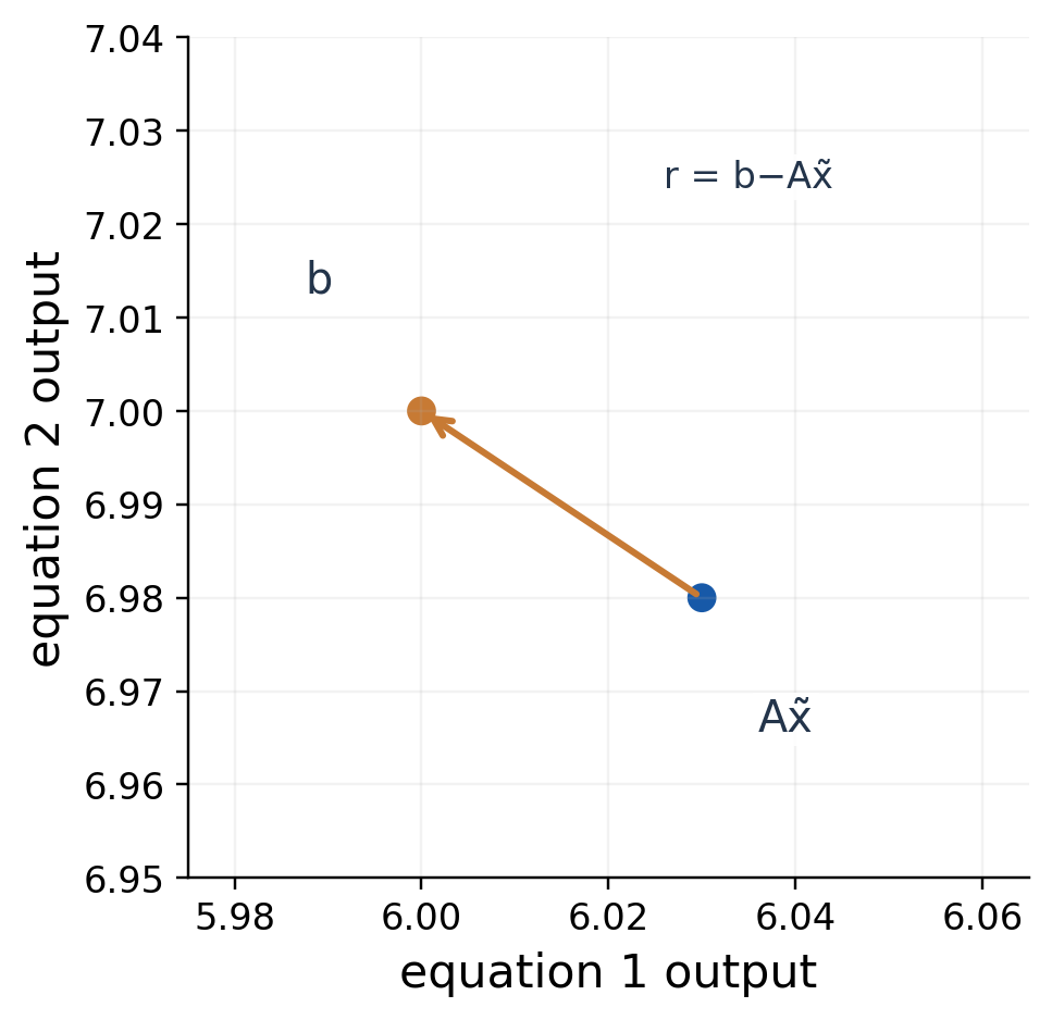
For A with rows (4,1),(1,3), b=(6,7)ᵀ and x̃=(1.01,1.99)ᵀ:
A x̃ = (6.03,6.98)ᵀ, r = (−0.03,0.02)ᵀ.
The largest absolute residual is 0.03. Here the exact solution is (1,2), so the largest component error is 0.01.

Worked Example 4.73 – Unequal Equation Scales
Let A=diag(1,10^(−8)), b=(1,10^(−8))ᵀ. The exact solution is (1,1)ᵀ. For x̃=(1,0)ᵀ, the residual is (0,10^(−8))ᵀ, yet the second component error is 1.
The second coefficient is tiny, so even a large variable error creates a small absolute equation mismatch. Scaling and conditioning therefore matter.
A scaled residual may compare ||r||∞ with ||A||∞||x̃||∞+||b||∞. The matrix infinity norm is the maximum absolute row sum. This helps compare magnitudes but does not remove ill-conditioning.
Retain guard digits during calculations. A result rounded too early can have a noticeably different residual from the working approximation.
Numerical Report
Give the approximation, its residual and the tolerance. A small change between iterations is useful information but is not an independent equation check.
Worked Example 4.74 – A Scaled Residual
For the displayed approximation, ||A||∞=5, ||x̃||∞=1.99, ||b||∞=7 and ||r||∞=0.03. Therefore:
||r||∞/(||A||∞||x̃||∞+||b||∞) = 0.03/16.95 = 1/565.
This dimensionless mismatch is about 0.00177. It supplements the raw residual and still does not independently bound solution error without sensitivity information.
26. Gauss–Seidel Iteration
Rearrange equation i to isolate variable i. During each sweep, use every newly computed component immediately in later equations.
xᵢ^(k+1) = [bᵢ−Σ(j<i) aᵢⱼxⱼ^(k+1)−Σ(j>i) aᵢⱼxⱼ^(k)]/aᵢᵢ.
The first sum uses new values and the second uses old values. All diagonal entries used in division must be nonzero.
Worked Example 4.75 – Isolate the Variables
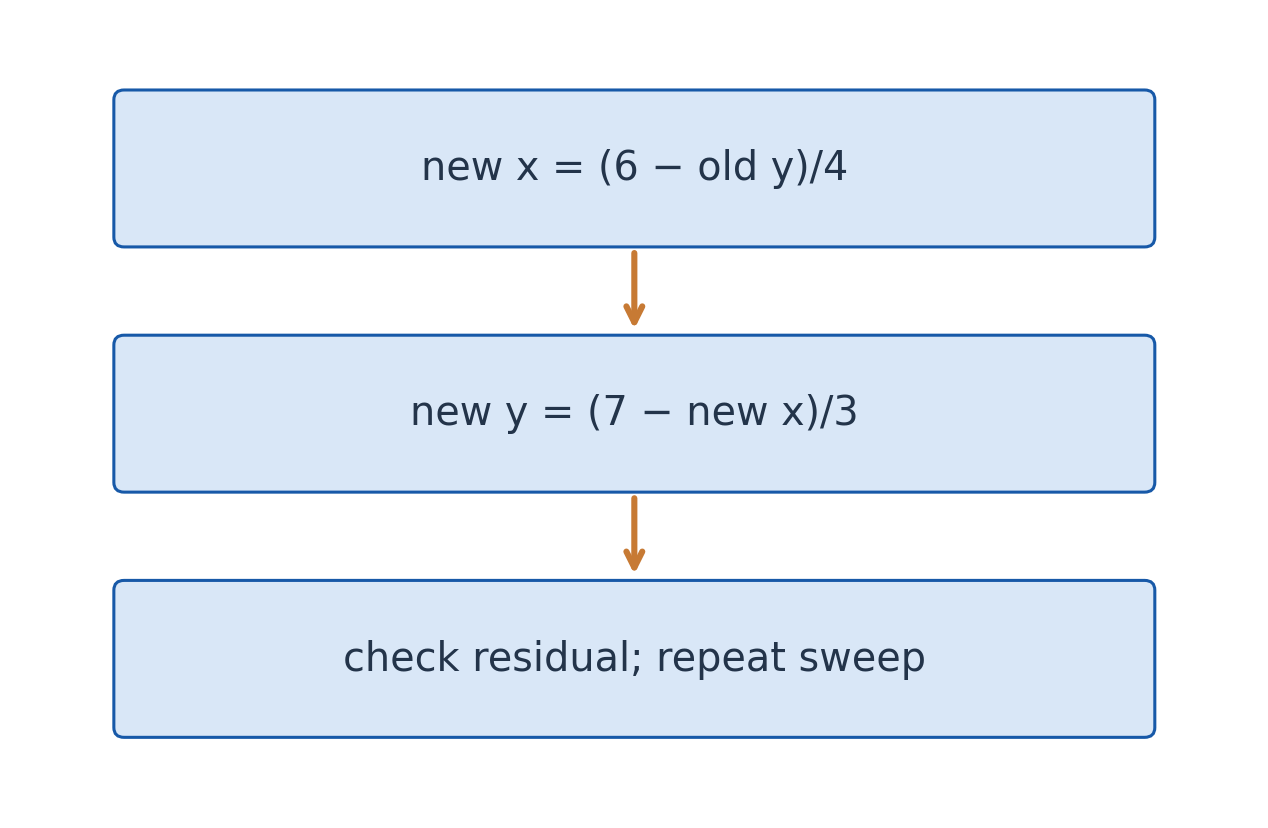
For 4x+y=6, x+3y=7:
x^(k+1) = (6−y^(k))/4.
y^(k+1) = (7−x^(k+1))/3.
From (0,0), first x=1.5, then y=11/6. The result is an approximation, not yet the exact solution.
Worked Example 4.76 – Matrix Form of One Sweep
For the two-variable system the updates can be collected as:
x_new = T x_old+c.
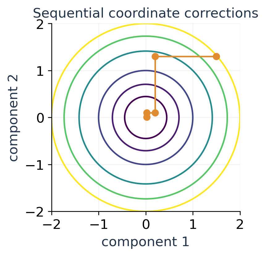
T = [[0,−1/4],[0,1/12]], c = (3/2,11/6)ᵀ.
Its eigenvalues are 0 and 1/12. The second update already incorporates the new first component; T therefore differs from the Jacobi matrix.

Jacobi uses only the previous sweep’s values for every component. The methods can have different convergence rates and ordering effects.
Iteration Procedure
- Step 1: Choose and state an equation and variable order.
- Step 2: Check the diagonal and a convergence condition.
- Step 3: State the initial vector.
- Step 4: Perform sequential updates with guard digits.
- Step 5: Check residual and stopping criteria.
Strict row diagonal dominance and real symmetric positive definiteness are useful sufficient convergence conditions. Nonsingularity alone is not sufficient.
Direct Versus Iterative
Elimination solves by a finite algebraic reduction. Iteration constructs a sequence and needs a justified convergence or failure assessment.
27. Gauss–Seidel: Two Variables
Worked Example 4.77 – Three Sweeps
Solve 4x+y=6, x+3y=7 from (0,0). Each diagonal magnitude exceeds its row’s off-diagonal sum.
The first sweep is x₁=3/2,y₁=11/6. The second gives:
x₂ = (6−11/6)/4 = 25/24, y₂ = 143/72.
The third gives:
x₃ = 289/288, y₃ = 1727/864.
Iteration Table
| Sweep | x | y |
|---|---|---|
| 0 | 0 | 0 |
| 1 | 1.500000 | 1.833333 |
| 2 | 1.041667 | 1.986111 |
| 3 | 1.003472 | 1.998843 |
Error and Sequential Geometry
The exact solution is (1,2). The y-error obeys:
e_y^(k+1) = (1/12)e_y^(k).
Thus each full sweep reduces this error by a factor 1/12 for this ordering. The x-error uses the preceding y-error.


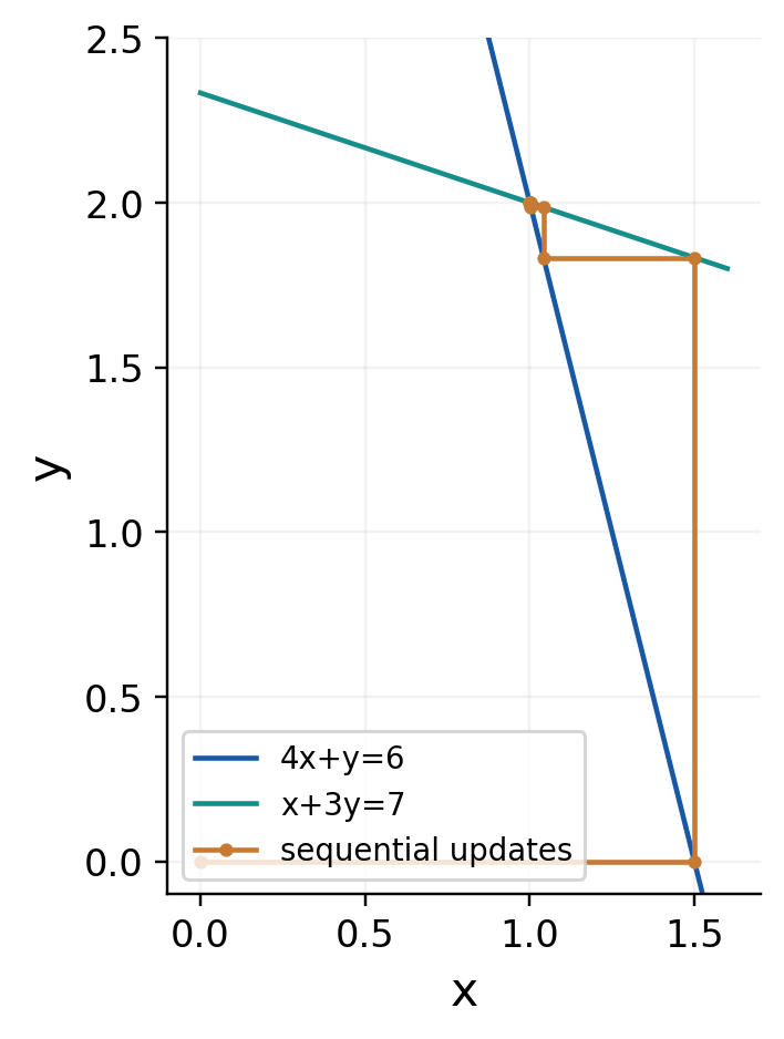
The second equation is satisfied exactly after a full sweep in exact arithmetic, because y was just computed from it. The first equation generally still has a residual.
A table rounded to three decimals can look unchanged before a stricter tolerance is met. Stop using unrounded working values, not visual equality of rounded table entries.
Latest Values
Use x_new in the y formula. Using x_old silently changes the algorithm to a different update rule.
Worked Example 4.78 – Third-Sweep Error
Subtract the exact solution (1,2) from the third pair:
e^(3) = (1/288,−1/864)ᵀ.
The maximum component error is 1/288≈0.003472. This is not equal to the maximum residual 11/864. Error and residual live in different spaces and are connected by multiplication with A.
28. Gauss–Seidel: Three Variables
Worked Example 4.79 – Form the Updates
10x+y+z=12.
2x+10y+z=13.
2x+2y+10z=14.
The updates are:
x_(k+1) = (12−y_k−z_k)/10.
y_(k+1) = (13−2x_(k+1)−z_k)/10.
z_(k+1) = (14−2x_(k+1)−2y_(k+1))/10.
All three rows are strictly diagonally dominant. Starting from zero gives x₁=1.2,y₁=1.06,z₁=0.948.
Worked Example 4.80 – Third Sweep with Guard Digits
The third working values are:
x₃ = 0.9995552, y₃ = 1.00018016.
z₃ = 1.000052928.
They are rounded in the table. Retaining these extra digits keeps the final residual calculation meaningful and prevents an apparently exact row from acquiring artificial rounding mismatch.
Continue in the Same Order
| Sweep | x | y | z |
|---|---|---|---|
| 0 | 0 | 0 | 0 |
| 1 | 1.200000 | 1.060000 | 0.948000 |
| 2 | 0.999200 | 1.005360 | 0.999088 |
| 3 | 0.999555 | 1.000180 | 1.000053 |
The exact solution is (1,1,1), giving constants 12,13,14 on substitution.
Worked Example 4.81 – Second Sweep Explicitly
First:
x₂ = (12−1.06−0.948)/10 = 0.9992.
Then:
y₂ = [13−2(0.9992)−0.948]/10 = 1.00536.
z₂ = [14−2(0.9992)−2(1.00536)]/10 = 0.999088.
The y-update uses new x and old z. The z-update uses both new x and new y. Changing this convention changes the sequence.
The table is rounded for display, while the computations retain additional digits. A different equation order can alter the rate of convergence and must be tracked consistently.
Three-Value Audit
At every update, identify which components are from this sweep and which are from the previous one. Do not update all three simultaneously using only old values.
Worked Example 4.82 – Residual After the Third Sweep
Using the working values rather than rounded table entries:
r = (0.004214912,−0.000964928,0)ᵀ.
The last equation is satisfied because z was just updated from it. Earlier equations generally are not exact after that z change. The largest absolute residual is 0.004214912, so a 0.001 residual tolerance would require further sweeps.
29. Convergence and Ordering
Strict row diagonal dominance means:
|aᵢᵢ| > Σ(j≠i) |aᵢⱼ| for every i.
It guarantees Gauss–Seidel convergence from every start. It is sufficient, not necessary; failure of the test does not alone prove divergence.
Worked Example 4.83 – Check the 3×3 System
The diagonal entries are 10 and the off-diagonal row sums are 2,3,4. Every row passes.
Real symmetric positive definite matrices provide another sufficient condition. Positive diagonal entries alone do not establish positive definiteness. For a symmetric 2×2 matrix, positive first leading minor and positive determinant suffice.
Worked Example 4.84 – Swap Equations
The system x+2y=3, 2x+y=3 is not diagonally dominant in its original order. Swap the rows:
2x+y=3, x+2y=3.
Now updates x_new=(3−y_old)/2 and y_new=(3−x_new)/2 converge. From zero the first two sweeps are (1.5,0.75) and (1.125,0.9375).

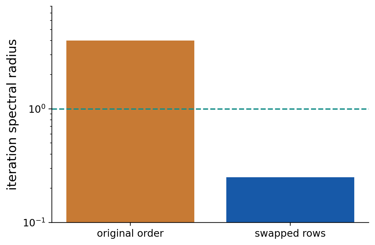
Not every matrix can be made diagonally dominant by row swaps. If a sufficient test fails, use another justified method or inspect the iteration matrix.
For fixed error iteration e_new=T e_old, convergence for every starting error is equivalent to spectral radius ρ(T)<1.
Test Logic
A sufficient condition passing proves convergence. The same condition failing leaves the question open until another argument settles it.
Positive Diagonals Are Insufficient
The symmetric matrix:
A = [[2,4],[4,3]].
has positive diagonal entries but determinant 6−16=−10. It is not positive definite. The symmetric-positive-definite convergence condition therefore cannot be inferred just by looking at the diagonal signs. Check the appropriate quadratic-form or leading-minor condition.
30. Stopping Criteria
Check both iterate changes and an independent equation residual:
Δ_k = ||x^(k+1)−x^(k)||∞.
r^(k+1) = b−Ax^(k+1).
Use scaled criteria when magnitudes differ substantially. State a tolerance rather than declaring an approximation “exact.”
Worked Example 4.85 – Third-Sweep Residual
For x₃=289/288,y₃=1727/864 in the two-variable example:
r₁ = 6−4x₃−y₃ = −11/864, r₂ = 0.
The maximum absolute residual is about 0.012731. A residual tolerance 0.001 has not yet been met.
A Contraction-Based Error Bound
If the iteration matrix has a known induced norm at most q<1, the current error can be bounded by q/(1−q) times the latest step change.
For the two-variable T, ||T||∞=1/4. The third-sweep step has maximum size 11/288, giving:
||e^(3)||∞ ≤ (1/4)/(1−1/4) = 11/864.
The actual error 1/288 satisfies this bound. This estimate needs the contraction hypothesis; it is not a universal step test.
Worked Example 4.86 – Another Sweep
x₄ = 3457/3456, y₄ = 20735/10368.
The first residual becomes −11/10368≈−0.001061, still slightly above 0.001 in magnitude. A fifth sweep reduces it by another factor 1/12 and meets this threshold.
Small changes can mean genuine convergence, slow progress or rounding stagnation. A step test alone cannot distinguish them.
Keep enough working digits to evaluate the residual honestly. Printed six-decimal values should not be used to claim twelve-digit accuracy.
A practical calculation also has a maximum sweep count and reports failure if a convergence test is not achieved. Failure of this iteration is not proof that the linear system has no solution.
Numerical Answer
Give the initial guess, update order, tolerance, final approximation and residual. These make the result independently reproducible.
Absolute and Relative Tolerances
A tolerance of 0.001 has a different relative meaning for a variable near one than for a variable near one million. Practical checks often combine absolute and relative thresholds.
The tolerance should match the problem’s units and accuracy needs. Do not tighten it below the accuracy supported by rounded inputs or working arithmetic merely to print more digits.
31. A Divergent Gauss–Seidel Example
Worked Example 4.87 – Nonsingular but Divergent
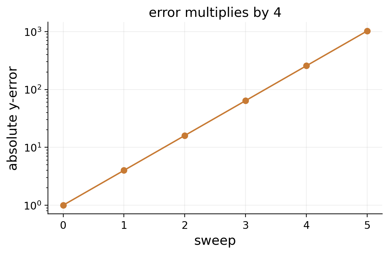
In the original equation order x+2y=3,2x+y=3:
x_(k+1) = 3−2y_k, y_(k+1) = 3−2x_(k+1).
Starting from zero gives (3,−3), then (9,−15), then (33,−63). The unique exact solution is (1,1), but the iteration moves away.
The y-error multiplies by 4 per sweep. Magnitude greater than one explains the growth.

Worked Example 4.88 – An Exceptional Starting Vector
Starting the divergent-order iteration exactly at (1,1) leaves it fixed, because it already solves both equations.
This does not establish convergence from arbitrary starts. The iteration matrix still has an error mode growing by four. The condition ρ(T)<1 concerns convergence for every initial error, not the trivial case of starting at the exact solution.
Direct and Iterative Methods
| Feature | Gauss Elimination | Gauss–Seidel |
|---|---|---|
| Process | Reduction and substitution | Sequential repeated sweeps |
| Initial guess | Not required | Required |
| Convergence test | Not an iterative issue | Essential |
| Verification | Original equations | Residual and tolerance |
Worked Example 4.89 – Repair the Ordering
Swapping the two equations leaves the exact solution fixed but changes the iteration error factor to 1/4. The earlier reorder therefore converges.
A zero diagonal prevents the standard isolated-variable update. A suitable reorder may fix it; if not, use another formulation or method.
A few improving iterates do not establish a universal convergence theorem. For a fixed linear iteration, ρ(T)<1 is the reliable every-start condition; norm behaviour can be more complicated over the first few steps.
Separate Claims
Nonsingularity, convergence of a chosen iteration, and meeting a printed tolerance are different facts. Verify each statement that is needed.
32. Eigenvalues and Eigenvectors
For square A, an eigenvector v≠0 and eigenvalue λ satisfy:
Av = λv.
The output remains on the same line as v. It may grow, shrink, reverse, or vanish. The zero vector is excluded because it satisfies the equation for every λ.
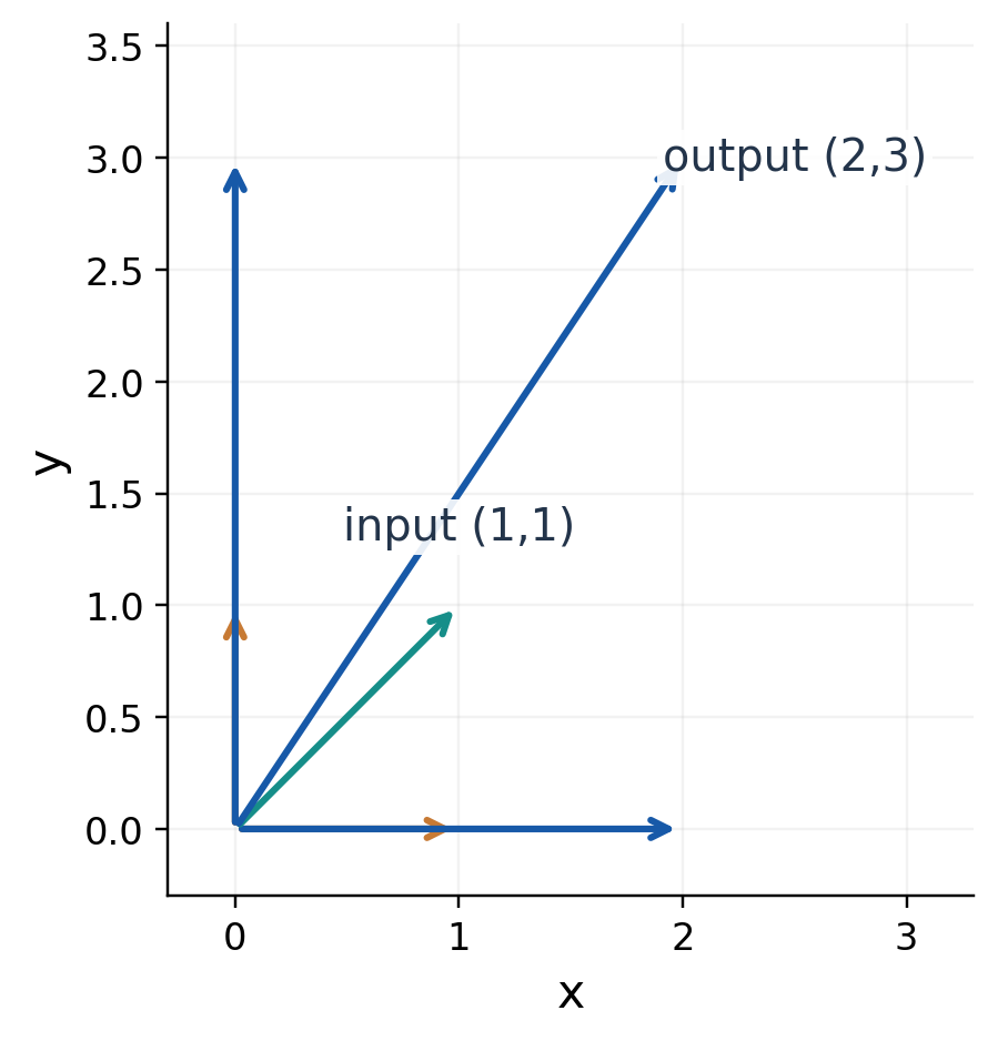
Worked Example 4.90 – A Diagonal Matrix
For A=diag(2,3), e₁ and e₂ have eigenvalues 2 and 3. But (1,1)ᵀ maps to (2,3)ᵀ, which is not a scalar multiple of it.

Characteristic Equation
A nonzero solution to (A−λI)v=0 exists when:
det(A−λI) = 0.
Find the roots, then solve the corresponding homogeneous systems. Roots alone do not supply eigenvectors.
Worked Example 4.91 – Zero Eigenvalue
For diag(1,0), the y-axis contains nonzero eigenvectors with λ=0. Zero may be an eigenvalue, although the zero vector cannot be an eigenvector.
A square matrix is singular exactly when zero is an eigenvalue. For any eigenvector, a nonzero scalar multiple gives another for the same eigenvalue.
A real matrix may have complex eigenvalues. The appropriate field matters when asking whether a complete real eigenvector basis exists.
Eigenpair Check
After solving the characteristic equation, verify Av=λv for each selected nonzero vector. Keep the vector paired with the value used in its null system.
Worked Example 4.92 – A Scalar Matrix
For cIₙ, every nonzero vector has eigenvalue c because cIₙv=cv. The characteristic polynomial has the repeated root c with multiplicity n, while the eigenspace has dimension n.
This supplies a simple example where repeated eigenvalues cause no diagonalisation difficulty. The nonzero-vector condition remains essential even when all directions qualify.
33. A Full 2×2 Eigenproblem
Worked Example 4.93 – Find the Roots
A = [[4,1],[2,3]].
det(A−λI) = (4−λ)(3−λ)−2.
det(A−λI) = λ²−7λ+10 = (λ−5)(λ−2).
The roots are 5 and 2. Their sum 7 matches trace(A), and their product 10 matches det A.
For λ=5, −x+y=0, so choose v₁=(1,1)ᵀ. Then Av₁=(5,5)ᵀ=5v₁.
The General 2×2 Characteristic Formula
For A with rows (a,b),(c,d):
det(λI−A) = λ²−(a+d)λ+(ad−bc).
For the stated A, trace is 7 and determinant 10, giving λ²−7λ+10. Substituting λ=5 yields 25−35+10=0; λ=2 gives 4−14+10=0. Checking roots independently helps catch a faulty factorisation.
Find the Second Eigendirection
For λ=2, solve 2x+y=0 and choose v₂=(1,−2)ᵀ:
A(1,−2)ᵀ = (2,−4)ᵀ = 2(1,−2)ᵀ.
The two vectors are independent because their column matrix has determinant −3.


Using det(λI−A) gives the same characteristic roots. In odd size it differs by an overall sign from det(A−λI), which does not affect zeros.
When assembling a diagonalisation, λ=5 must remain paired with v₁ and λ=2 with v₂. Interchanging only the values or only the columns gives a wrong factorisation.
Verification
Direct multiplication of two small eigenvectors is often faster than searching a long determinant expansion for an unnoticed sign error.
Worked Example 4.94 – Rescale an Eigenvector
Replace v₂=(1,−2)ᵀ by w=(3,−6)ᵀ. Then:
Aw = (6,−12)ᵀ = 2w.
The same eigendirection remains valid. Only multiplying by zero would invalidate the vector. An eigenvector answer is not unique in magnitude; a normalisation requirement must be stated separately.
34. A 3×3 Eigenproblem
Worked Example 4.95 – A Triangular Matrix
A = [[2,1,0],[0,3,1],[0,0,4]].
The triangular determinant has factors 2−λ,3−λ,4−λ. The eigenvalues are 2,3,4.
For λ=2, the last equations give z=y=0; choose v₁=(1,0,0)ᵀ. For λ=3, z=0 and y=x; choose v₂=(1,1,0)ᵀ.
For λ=4, y=2x and z=y; choose v₃=(1,2,2)ᵀ.
Av₁=2v₁, Av₂=3v₂, Av₃=4v₃.
Worked Example 4.96 – Inspect the λ=3 Null System
A−3I = [[−1,1,0],[0,0,1],[0,0,1]].
The last rows repeat z=0, while the first gives y=x. Rank is two, leaving one free direction (t,t,0). A nonzero choice t=1 gives v₂. This is why the eigenvector is not simply the second coordinate unit vector.
Independent Eigenvectors
Eigenvectors for distinct eigenvalues are independent. Assemble the columns in the same order:
S = [[1,1,1],[0,1,2],[0,0,2]], D = diag(2,3,4).
Since det S=2, it is invertible.
Worked Example 4.97 – Verify the Third Vector
A(1,2,2)ᵀ = (4,8,8)ᵀ = 4(1,2,2)ᵀ.
Triangular form makes eigenvalues easy, but does not make all coordinate unit vectors eigenvectors. Here e₂ maps to (1,3,0)ᵀ, not 3e₂. Off-diagonal coupling still affects eigendirections.
The eigenvector matrix will diagonalise A later. Checking AS=SD uses the same three verified column equations.
Triangular Shortcut
Read eigenvalues from a triangular diagonal, but solve eigenvectors from the full matrix. Do not ignore off-diagonal entries in the null systems.
Trace and Determinant Cross-Check
The eigenvalue sum 2+3+4=9 equals the diagonal trace. The product 2×3×4=24 equals the triangular determinant.
det(λI−A) = λ³−9λ²+26λ−24.
The coefficient 26 is 2×3+2×4+3×4. These checks use the original matrix, whose off-diagonal entries still determine its eigenvectors.
35. Repeated Roots and Defectiveness
Algebraic multiplicity counts how often λ occurs as a characteristic root. Geometric multiplicity is the dimension of its eigenspace. A repeated root does not automatically provide enough independent eigenvectors.
Worked Example 4.98 – Repeated but Diagonalizable
For 2I₂, the only root is 2 with multiplicity two. Every nonzero vector is an eigenvector, so two independent ones can be selected.
Worked Example 4.99 – A Defective Matrix
J = [[2,1],[0,2]].
The root 2 has multiplicity two, but (J−2I)v=0 gives y=0. Only one eigendirection exists, and J is not diagonalizable.


Count Eigenspace Dimensions
For each eigenvalue, geometric multiplicity lies between one and its algebraic multiplicity. Diagonalisation requires n independent eigenvectors altogether.
Worked Example 4.100 – A Repeated 3×3 Root
For diag(2,2,3), the λ=2 eigenspace consists of (x,y,0) and has dimension two. Together with (0,0,1), it provides a complete basis.
Copying the same eigenvector twice gives a singular column matrix; it does not create the missing direction.
A defective block may also create polynomial growth factors in repeated updates. For eigenvalues strictly inside the unit circle these can still decay, but at a unit-circle boundary they can destroy bounded stability.
Repeated-Root Method
For every repeated λ, row-reduce A−λI and count independent free directions. Do not decide diagonalisation from the characteristic polynomial alone.
Worked Example 4.101 – Defective Powers Differ
Write the defective J as 2I+N with N having only upper-right entry one. Since N²=0:
J² = 4I+4N = [[4,4],[0,4]].
This differs from the square of 2I. Equal repeated eigenvalues do not make the matrices identical or give them equal powers. Their eigenspace structure matters.
36. Eigenvalue Properties
Counting algebraic multiplicities:
Σᵢλᵢ = tr A, Πᵢλᵢ = det A.
Transpose preserves the characteristic polynomial. Triangular matrices have their diagonal entries as eigenvalues.
Worked Example 4.102 – Check a Proposed Pair
For A with rows (4,1),(2,3), 5 and 2 sum to 7 and multiply to 10. The proposed pair 4,3 has the same sum but wrong product, so it fails.
Worked Example 4.103 – Shift by Identity
If Av=λv, then:
(A+cI)v = (λ+c)v.
Adding 2I changes the eigenvalues 5,2 to 7,4 while preserving those eigendirections.
Worked Example 4.104 – Check the Inverse Spectrum
For A with rows (4,1),(2,3):
A⁻¹ = (1/10)[[3,−1],[−2,4]].
Its trace is 7/10=1/5+1/2 and determinant is 1/10=(1/5)(1/2). These agree with reciprocal eigenvalues. Trace of inverse is not generally reciprocal trace; it is the sum of reciprocal eigenvalues.
Powers, Reciprocals and Conjugate Pairs
If Av=λv:
Aᵏv = λᵏv for nonnegative integer k.
If A is invertible:
A⁻¹v = (1/λ)v.
Worked Example 4.105 – Inverse Spectrum
The inverse of the same A has eigenvalues 1/5 and 1/2 with the same eigenvectors. A zero eigenvalue prevents an ordinary inverse, so no reciprocal rule applies there.
A real characteristic polynomial has nonreal roots in conjugate pairs. A general complex matrix need not have that property.
Taking determinants in U†U=I gives |det U|²=1, so a unitary determinant has modulus one. This is necessary but not sufficient for unitarity.
Trace and determinant checks are useful, but do not replace solving eigenspaces. Different matrices can share their spectrum and still have different eigendirections or diagonalisation properties.
Field Check
State whether eigenvectors and coordinate changes are allowed to be complex. A real matrix can fail real diagonalisation while admitting a complex one.
Worked Example 4.106 – Conjugate Rotation Roots
For a 90° real rotation, trace is zero and determinant one. The roots i and −i satisfy:
i+(−i)=0, i(−i)=1.
They are conjugates and lie on the unit circle. Real coefficients force pairing, while orthogonality forces unit modulus. These are two separate structural explanations.
37. Spectra of Complex Matrix Classes


Worked Example 4.107 – A Hermitian Eigenproblem
H = [[2,i],[−i,2]].
Its characteristic equation is (2−λ)²−1=0, giving 3,1. Choose v₁=(i,1)ᵀ and v₂=(−i,1)ᵀ.
v₁†v₂ = (−i)(−i)+1 = 0.
Both have norm √2; dividing by it gives an orthonormal set.
A Unitary Eigenvector Matrix
For the Hermitian example, normalise both vectors:
U = (1/√2)[[i,−i],[1,1]].
Its columns have norm one and zero mutual complex inner product. This permits unitary, rather than merely invertible, diagonalisation.
Worked Example 4.108 – Multiply by i
K=iH is skew-Hermitian with eigenvalues 3i and i. Its eigenvectors stay the same because scalar multiplication scales the eigenvalues.
Worked Example 4.109 – A Real Rotation
R = [[0,−1],[1,0]], λ²+1=0.
The roots are i and −i. No nonzero real line is invariant under a 90° rotation, so real eigenvectors do not exist.
For λ=i, the complex vector (1,−i)ᵀ satisfies Rv=(i,1)ᵀ=iv. Complex eigendirections resolve what the real plane cannot supply.
Spectrum Check
A genuinely nonreal eigenvalue for a Hermitian matrix signals a calculation or classification error. Real entries alone do not imply real eigenvalues; real symmetry does.
Worked Example 4.110 – Verify the Complex Diagonal Form
With that ordered U:
U†HU = [[3,0],[0,1]].
Ordinary transpose would not replace U† here because its columns contain imaginary entries. The correct adjoint retains both orthogonality and the real eigenvalue interpretation.
38. Similarity Transformations
A and B are similar if an invertible S satisfies:
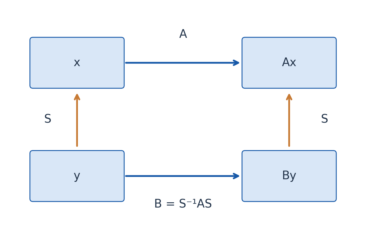
B = S⁻¹AS.
They describe one linear transformation in different coordinate bases. Similarity preserves eigenvalues, characteristic polynomial, determinant, trace and rank.
Worked Example 4.111 – Compute a Similarity
A = [[2,0],[0,3]], S = [[1,1],[0,1]].
S⁻¹ = [[1,−1],[0,1]], B = [[2,−1],[0,3]].
Direct multiplication gives B=S⁻¹AS. Both matrices have eigenvalues 2,3, trace 5 and determinant 6, although only A is diagonal.

Similarity Is Not Row Equivalence
If x=Sy, the update x_new=Ax becomes y_new=S⁻¹AS y. Both inverse and forward coordinate factors are needed.
Row operations preserve rank but usually change eigenvalues. Scaling row 1 of diag(2,3) by 2 gives diag(4,3), a changed spectrum. Reading eigenvalues from an echelon form is therefore generally invalid.
Worked Example 4.112 – Transform an Eigenvector
If Av=λv and w=S⁻¹v:
Bw = S⁻¹Av = λw.
Eigenvalues stay the same while eigenvector coordinates change.
An arbitrary similarity need not preserve Euclidean lengths or symmetry of the displayed matrix. Orthogonal and unitary coordinate changes preserve additional geometric structure.
Order Check
S must be invertible, and B must contain both S⁻¹ and S in the correct order. Multiplication on only one side is not similarity.
Worked Example 4.113 – New Coordinates of an Eigenvector
For the similarity example, take v=(0,1)ᵀ, an eigenvector of A for λ=3. Then w=S⁻¹v=(−1,1)ᵀ.
Bw = (−3,3)ᵀ = 3w.
The vector’s coordinate entries changed, but its eigenvalue did not. This makes the basis-change interpretation concrete rather than merely a three-factor matrix identity.
39. Diagonalisation
A full set of independent eigenvectors forms an invertible S with:
S⁻¹AS = D, A = SDS⁻¹.
D’s diagonal entries match the corresponding columns of S.
Worked Example 4.114 – A 2×2 Diagonalisation
For A with rows (4,1),(2,3), take λ₁=5,v₁=(1,1)ᵀ and λ₂=2,v₂=(1,−2)ᵀ:
S = [[1,1],[1,−2]], D = diag(5,2).
S⁻¹ = (1/3)[[2,1],[1,−1]].
The determinant of S is −3, so the inverse exists.

Verify with Column Equations
Instead of multiplying three full matrices, check AS=SD:
AS = [[5,2],[5,−4]] = SD.
Each column is its eigenvector equation. Multiplication by S⁻¹ establishes the diagonal form.
Worked Example 4.115 – Change Column Order
If S uses v₂,v₁ instead, D must become diag(2,5). Reordering only one breaks the factorisation.
Eigenvector columns need not have unit length for ordinary diagonalisation. Any nonzero column scaling is valid if S and its inverse are used consistently.
A defective matrix cannot provide n independent eigenvectors, so every attempted complete eigenvector matrix is singular. Repeated roots alone do not cause failure; insufficient eigenspace dimension does.
Pairing Habit
Record each λ beside its eigenvector before assembling S. Verify the column order and det S≠0 before using S⁻¹.
Another Verification Route
For the selected S and A:
S⁻¹A = (1/3)[[10,5],[2,−2]] = DS⁻¹.
Multiplying on the right by S gives the same diagonal form. Both AS=SD and S⁻¹A=DS⁻¹ express the eigenvector factorisation. Choose the shorter check rather than recomputing every product without structure.
40. A 3×3 Diagonalisation
Worked Example 4.116 – Assemble the Known Eigenpairs
A = [[2,1,0],[0,3,1],[0,0,4]].
For λ=2,3,4 use v₁=(1,0,0)ᵀ,v₂=(1,1,0)ᵀ,v₃=(1,2,2)ᵀ:
S = [[1,1,1],[0,1,2],[0,0,2]], D = diag(2,3,4).
S⁻¹ = [[1,−1,1/2],[0,1,−1],[0,0,1/2]].
Each inverse entry can be checked by SS⁻¹=I. The determinant of S is 2.
Worked Example 4.117 – Decompose an Ordinary Vector
For x=(3,1,2)ᵀ, the eigenvector coordinates are:
y = S⁻¹x = (3,−1,1)ᵀ.
Indeed 3v₁−v₂+v₃=(3,1,2)ᵀ. This demonstrates how an input that is not itself an eigenvector still splits into independent modal components.
Verification and Coordinates
AS = [[2,3,4],[0,3,8],[0,0,8]] = SD.
Hence S⁻¹AS=D.
Worked Example 4.118 – Coordinates of an Eigenvector
For x=(1,2,2)ᵀ, S⁻¹x=(0,0,1)ᵀ because x is exactly column 3. For x=(1,0,0)ᵀ the new coordinates are (1,0,0)ᵀ.
Distinct eigenvalues guaranteed independence here. Distinct roots are sufficient but not necessary for diagonalisation, as a diagonal matrix with repeated entries demonstrates.
If a real matrix has nonreal roots, it may diagonalise over the complex numbers but not the real numbers. The permitted field determines what counts as a valid basis.
Three-Column Audit
Verify each Avᵢ=λᵢvᵢ, check invertibility of S and then check AS=SD. This structured test is often simpler than a long unorganised product.
Worked Example 4.119 – Update Using Modal Coordinates
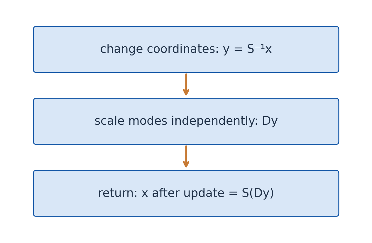
The preceding y becomes Dy=(6,−3,4)ᵀ. Returning to the original frame gives:
S(Dy) = (7,5,8)ᵀ = Ax.
The diagonal update and direct multiplication agree. This is the same transformation computed through two coordinate descriptions, not an approximation or a different model.
41. Powers Through Diagonalisation
Intermediate inverse factors cancel in repeated multiplication:
Aᵏ = SDᵏS⁻¹, k=0,1,2,…
Diagonal powers require only scalar powers.
Worked Example 4.120 – General Power Formula
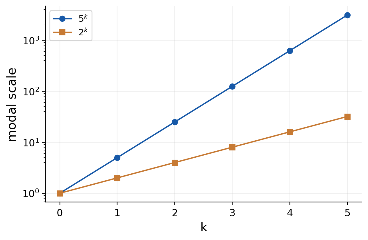
For A with rows (4,1),(2,3), write p=5ᵏ and q=2ᵏ. Then:
Aᵏ = (1/3)[[2p+q,p−q],[2p−2q,p+2q]].
At k=0 it gives I, and at k=1 it gives A. These simple tests check eigenvector pairing and inverse factors.

Worked Example 4.121 – A Squared
At k=2, p=25,q=4:
A² = [[18,7],[14,11]].
Direct multiplication gives 4×4+1×2=18 and 2×1+3×3=11 on the diagonal, agreeing with the formula.
Worked Example 4.122 – An Initial Modal Combination
If x₀=v₁+v₂, then:
x_k = 5ᵏv₁+2ᵏv₂.
The original coordinates are coupled, but the eigenvector coordinates evolve independently.
For invertible A, negative integer powers use the same factorisation with reciprocal diagonal powers. A zero eigenvalue cannot be raised to a negative power in an ordinary inverse formula.
Defective matrices do not admit this diagonal eigenvector formula. Their powers can include additional polynomial factors, particularly important at a stability boundary.
Power Check
Always test a general formula at k=0 and k=1 before using a large exponent.
42. Orthogonal Diagonalisation
Real symmetric matrices admit an orthonormal eigenvector basis:
QᵀAQ = D, Q⁻¹ = Qᵀ.
Worked Example 4.123 – A Symmetric Matrix
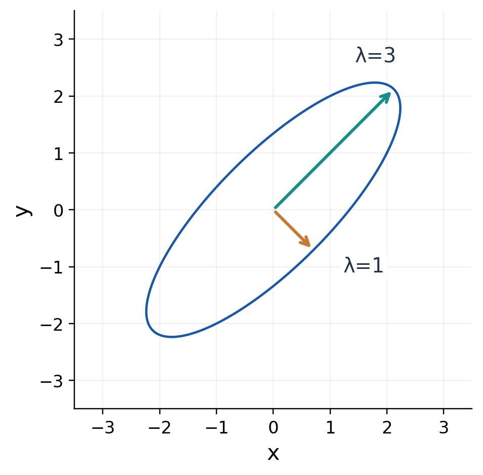
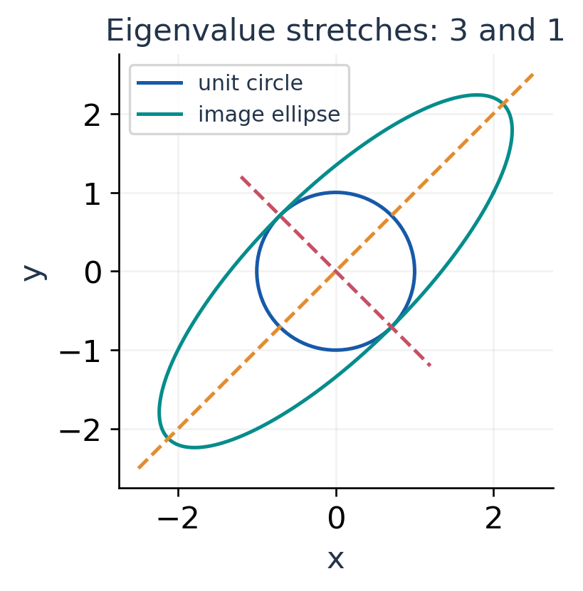
A = [[2,1],[1,2]].
Eigenvalues are 3,1 with directions (1,1),(1,−1). Normalise:
Q = (1/√2)[[1,1],[1,−1]], D = diag(3,1).
Then QᵀQ=I and QᵀAQ=D.

Quadratic Forms and Complex Extension
Writing x=Qy gives:
xᵀAx = yᵀDy = 3y₁²+y₂².
The mixed term disappears. Both eigenvalues are positive, so the quadratic form is positive for every nonzero x.
Worked Example 4.124 – Verify a Value
For x=(1,0)ᵀ, y=(1,1)ᵀ/√2. The diagonal expression gives 3/2+1/2=2, agreeing with xᵀAx.
Repeated eigenspaces may need an orthonormal choice within them; distinct-eigenvalue eigenvectors of a symmetric matrix are already perpendicular.
Hermitian matrices use unitary diagonalisation U†HU=D with real D. Ordinary transpose is replaced by conjugate transpose. General non-Hermitian matrices need not have a unitary eigenvector basis.
Inverse Shortcut
Q⁻¹=Qᵀ depends on orthogonality. An arbitrary eigenvector matrix S does not usually have its transpose as inverse.
Orthogonal Diagonal Does Not Mean Positive
The symmetric matrix diag(1,−1) is already orthogonally diagonal, but its quadratic form x²−y² takes either sign.
For (1,0) it equals one; for (0,1) it equals minus one. Positive definiteness requires positive eigenvalues in addition to symmetry. Orthogonal diagonalisation itself is available for every real symmetric matrix, including indefinite ones.

43. Discrete-Time Stability
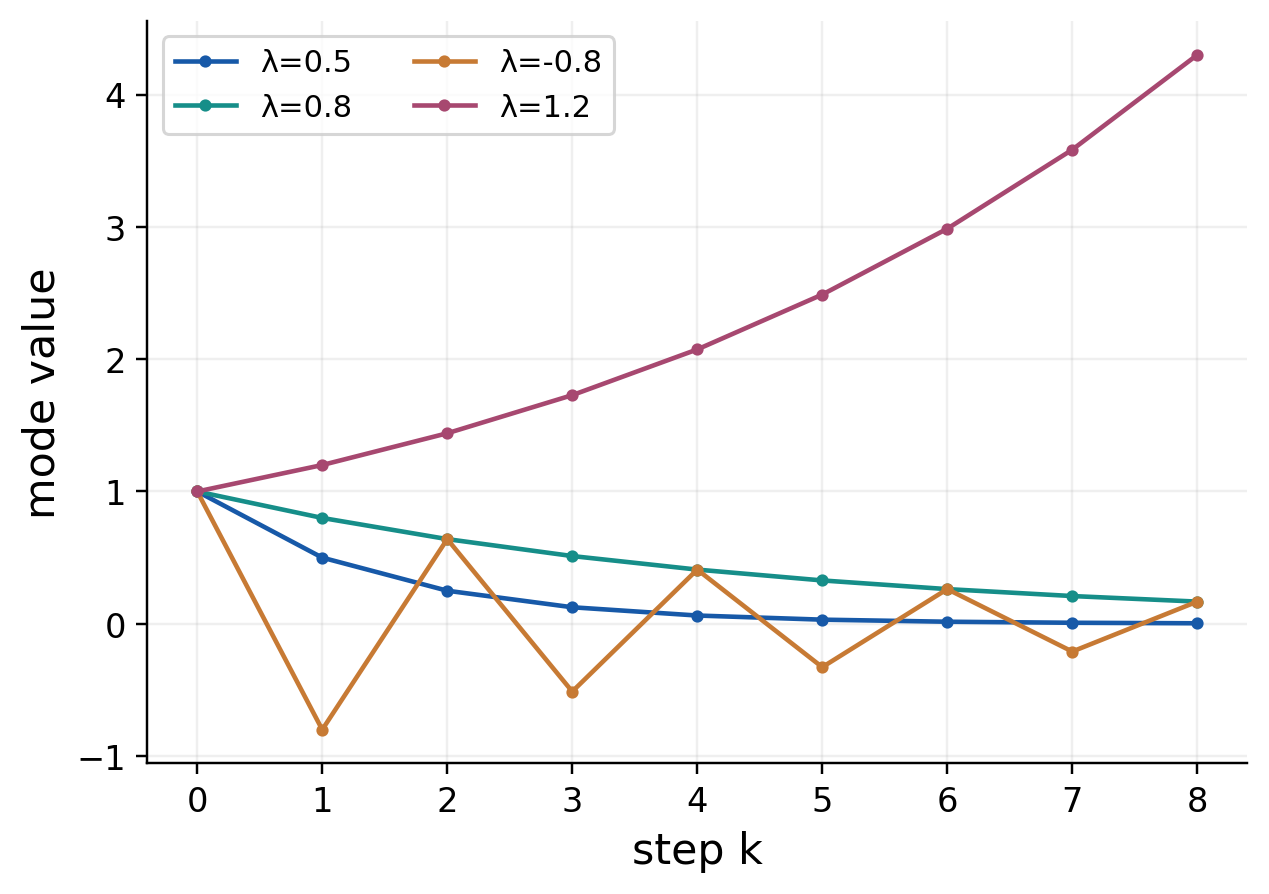
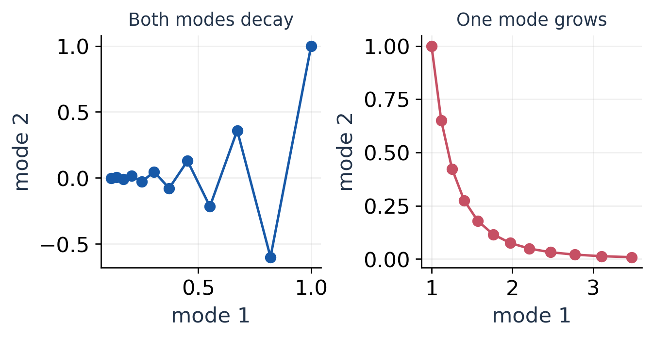
For x_(k+1)=Ax_k, x_k=Aᵏx₀. Modal components scale as λᵏ. If every |λ|<1, all states tend to zero and the origin is asymptotically stable. Any |λ|>1 creates an unstable direction.
Worked Example 4.125 – Decaying Modes
For A=diag(1/2,4/5), the coordinates are (1/2)ᵏx₀ and (4/5)ᵏy₀. Both decay, with the second slower.

Worked Example 4.126 – Bounded but Not Decaying
For diag(1,1/2), the first coordinate stays constant and the second decays. The origin is stable but not asymptotically stable. A λ=−1 mode alternates without decay.
Worked Example 4.127 – Evaluate Three Updates
For the decaying diagonal matrix and x₀=(8,5)ᵀ:
x₃ = ((1/2)³8,(4/5)³5)ᵀ = (1,2.56)ᵀ.
Both coordinates are smaller, but the second remains larger because its mode decays more slowly. Long-term stability describes the limit as k grows; it does not require every coordinate to vanish after a small fixed number of steps.
Negative Is Not Automatically Unstable
A discrete mode λ=−0.8 alternates sign but its magnitude is 0.8ᵏ and decays. A positive mode λ=1.2 grows. Thus the sign alone is not the criterion: the unit-circle magnitude test determines decay, and boundary eigenstructure determines the remaining bounded cases.
Worked Example 4.128 – A Defective Unit Mode
J = [[1,1],[0,1]], Jᵏ = [[1,k],[0,1]].
From x₀=(0,1)ᵀ, x_k=(k,1)ᵀ grows without bound although both eigenvalues have modulus one.
For finite-dimensional linear dynamics, bounded stability with unit-circle modes requires those boundary eigenvalues to be semisimple: no defective block there. Defective blocks strictly inside the circle can still decay.
Gauss–Seidel error obeys e_new=T e_old. Its every-start convergence condition ρ(T)<1 is the same modal-decay principle applied to iteration error.
Stability Label
Specify discrete time and distinguish bounded behaviour from decay to zero. Spectral radius equal to one alone does not settle the boundary case.

44. Continuous-Time Stability
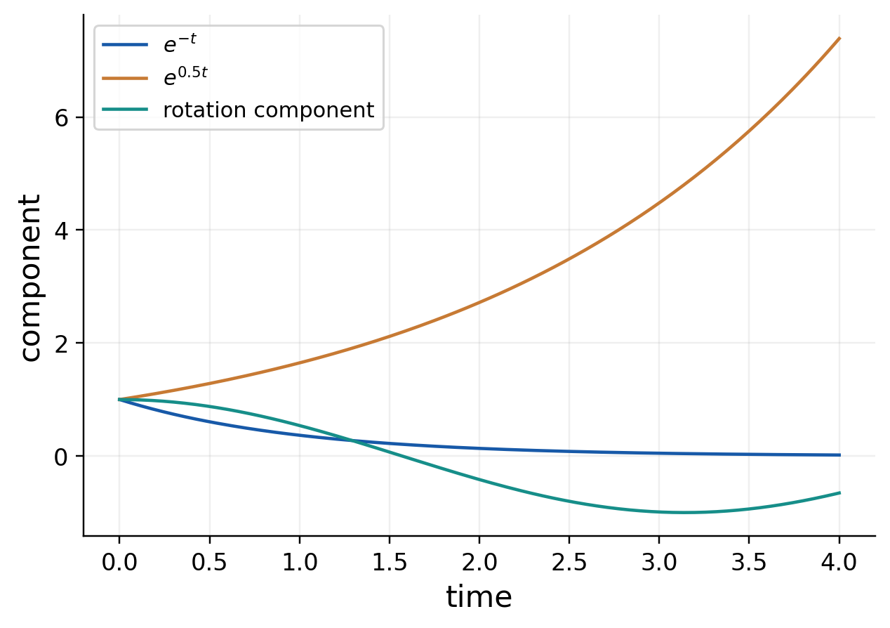
For x′(t)=Ax(t), an eigenmode evolves as e^(λt). Magnitude depends on Re λ. All negative real parts give asymptotic stability; any positive real part gives instability.
Worked Example 4.129 – Two Decays
For A=diag(−1,−3), coordinates are e^(−t)x₀ and e^(−3t)y₀. Both tend to zero, with the second faster.

Worked Example 4.130 – Rotation
For A with rows (0,−1),(1,0), eigenvalues ±i produce constant-norm rotation. The origin is stable but not asymptotically stable.
Worked Example 4.131 – A Convenient Observation Time
For A=diag(−1,−3) and x₀=(2,8)ᵀ, evaluate at t=ln 2:
x(t) = (2e^(−t),8e^(−3t))ᵀ.
x(ln 2) = (1,1)ᵀ.
The second starts larger but decays faster. This calculation checks both the initial-value factors and the continuous exponential law. Repeated integer powers of A would describe a different, discrete update problem.
Worked Example 4.132 – A Defective Zero Mode
N = [[0,1],[0,0]], e^(tN) = I+tN.
Initial state (0,1)ᵀ becomes (t,1)ᵀ and grows. Boundary eigenvalues with zero real part require a semisimplicity check for bounded stability.
The scalar λ=−2 is stable for x′=−2x, but unstable for x_(k+1)=−2x_k. Continuous time uses real parts; discrete time uses magnitudes.
For symmetric positive definite H, x′=−Hx decays. A discrete gradient step instead uses I−αH, whose eigenvalues must be placed inside the unit circle by choosing a suitable step size.
Separate Models
Do not reuse a continuous test for a sampled update matrix or vice versa. State the time model before interpreting eigenvalues.
45. Binary Error Detection
Coding uses arithmetic modulo 2, where 1+1=0. A parity-check matrix tests a received column r by syndrome s=Hr mod 2. A valid codeword c satisfies Hc=0.
Worked Example 4.133 – One Parity Equation
For H=(1,1,1), c=(1,0,1)ᵀ gives 1+0+1=0 mod 2. Flipping the second bit gives syndrome 1. The error is detected, but one parity bit cannot identify its position.


A nonzero syndrome identifies a violated check. Error correction needs additional structure and an explicitly stated error model.
Worked Example 4.134 – An Undetected Even Change
For the simple three-bit parity check, c=101 is valid. Flipping its first two bits gives 011, whose parity is also zero.
| Word | Sum mod 2 | Check |
|---|---|---|
| 101 | 0 | Pass |
| 111 | 1 | Fail |
| 011 | 0 | Pass |
A single parity equation detects every odd number of changes, but not every even pattern. More checks are needed for stronger guarantees.
A Seven-Bit Check Matrix
Use binary labels 1–7 as columns, least-significant-bit first:
H = [[1,0,1,0,1,0,1],[0,1,1,0,0,1,1],[0,0,0,1,1,1,1]].
Parity positions are 1,2,4 and data positions 3,5,6,7.
Worked Example 4.135 – Encode (1,0,1,1)
The parity equations give:
p₁ = 1+0+1 = 0 mod 2.
p₂ = 1+1+1 = 1 mod 2.
p₄ = 0+1+1 = 0 mod 2.
The codeword is:
c = (0,1,1,0,0,1,1)ᵀ.
Multiplication verifies Hc=(0,0,0)ᵀ mod 2. The sums 2 and 4 both have parity zero.
Field Matters
Coding row operations and rank are over the binary field. Do not copy ordinary real arithmetic into a modulo-2 calculation.
Verify the Encoded Word Row by Row
For c=0110011, the selected sums in H are 0+1+0+1, 1+1+1+1 and 0+0+1+1. All are even.
Hc = (0,0,0)ᵀ mod 2.
This verifies the parity placement independently of the construction formulas. The same bit order must be used in encoding, syndrome multiplication and error lookup.
46. Syndrome-Based Correction
If r=c+e mod 2, the syndrome is He. For a single changed bit j, e selects column j of H. Distinct nonzero columns therefore identify any single-bit error in this code.
Worked Example 4.136 – Correct Bit 6
Flip bit 6 of the previous codeword:
r = (0,1,1,0,0,0,1)ᵀ.
Hr = (0,1,1)ᵀ mod 2.
Least-significant-bit first, 0+2+4=6. Flip that position back to recover c.

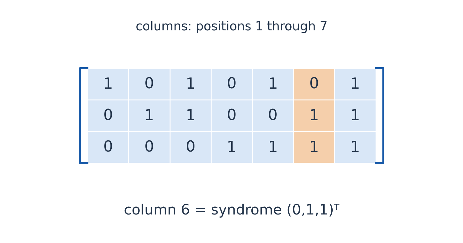
Syndrome Lookup Examples
| Changed Bit | Syndrome, Least Bit First |
|---|---|
| 1 | (1,0,0) |
| 2 | (0,1,0) |
| 6 | (0,1,1) |
| 7 | (1,1,1) |
The syndrome labels are columns of H, not arbitrary decimal-to-binary conventions. Writing the row order explicitly prevents reading (0,1,1) incorrectly as position 3 instead of 6.
State the Correction Assumption
This seven-bit code has minimum Hamming distance 3. It corrects one error and detects every two-bit error when used as an error-detection check.
A decoder blindly assuming one error can nevertheless miscorrect a two-bit pattern.
Worked Example 4.137 – A Misleading Syndrome
Errors in positions 1 and 2 give column 1+column 2=(1,1,0)ᵀ, equal to column 3. A single-error decoder would incorrectly flip bit 3.
Thus a nonzero syndrome detects failure of code membership but does not by itself distinguish one changed bit from two.
An additional overall parity check supports the standard single-error-correction, double-error-detection extension. That extra discrimination does not come for free from the original three-bit syndrome.
Decoder Claim
Column lookup is justified for one error. It is not guaranteed correction of an arbitrary corrupted word.
Why Minimum Distance Is Three
No one-bit word is a codeword because every H column is nonzero. No two-bit word is a codeword because distinct columns do not sum to zero over the binary field.
But bits 1,2,3 together do give zero syndrome, since column 1+column 2=column 3. Thus a nonzero codeword of weight three exists, establishing minimum distance exactly three.
47. Graphics: Linear Plane Transforms
Matrices transform vertices by scaling, rotation, reflection and shear. A collection of column vertices V can be transformed together as AV.
Worked Example 4.138 – Rotate a Point
R = [[0,−1],[1,0]].
It maps (2,1)ᵀ to (−1,2)ᵀ and preserves the norm √5 because RᵀR=I.
Worked Example 4.139 – Reflect a Point
The matrix diag(1,−1) maps (2,1)ᵀ to (2,−1)ᵀ. Determinant −1 records orientation reversal while preserving area magnitude.

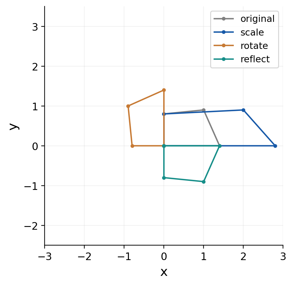
Composition and Coordinate Frames
For S=diag(2,1) and p=(1,1)ᵀ:
RSp = (−1,2)ᵀ, SRp = (−2,1)ᵀ.
The rightmost operation acts first for column vectors. Row-vector software conventions require the corresponding transposes and reversed order.
Worked Example 4.140 – Area-Preserving Shear
The matrix with rows (1,1),(0,1) moves the top of a unit square right by one and leaves the bottom fixed. Its determinant is one, but lengths and angles generally change. Area preservation is not orthogonality.
Local, world and camera coordinates are different frames. An arithmetically correct matrix used in the wrong frame can produce an incorrect rendered result.
Graphics Audit
Specify vector convention, coordinate frame and operation order. Test one known point before transforming the full vertex matrix.
Worked Example 4.141 – Transform Several Vertices
Put a triangle’s vertices into columns:
V = [[0,1,0],[0,0,1]].
RV = [[0,0,−1],[0,1,0]].
The origin stays fixed, the x-unit vertex moves to the y-unit vertex, and the y-unit vertex moves left. One matrix product transforms all columns using the same convention, which is useful for a mesh with many vertices.
48. Homogeneous Graphics Coordinates
Translation moves the origin, so it is not an ordinary 2×2 linear map. Represent (x,y) by (x,y,1)ᵀ and use 3×3 affine matrices.
Worked Example 4.142 – Translate a Point
T = [[1,0,3],[0,1,−1],[0,0,1]].
T(1,2,1)ᵀ = (4,1,1)ᵀ.
A direction has last coordinate zero, so the same translation leaves it unchanged.

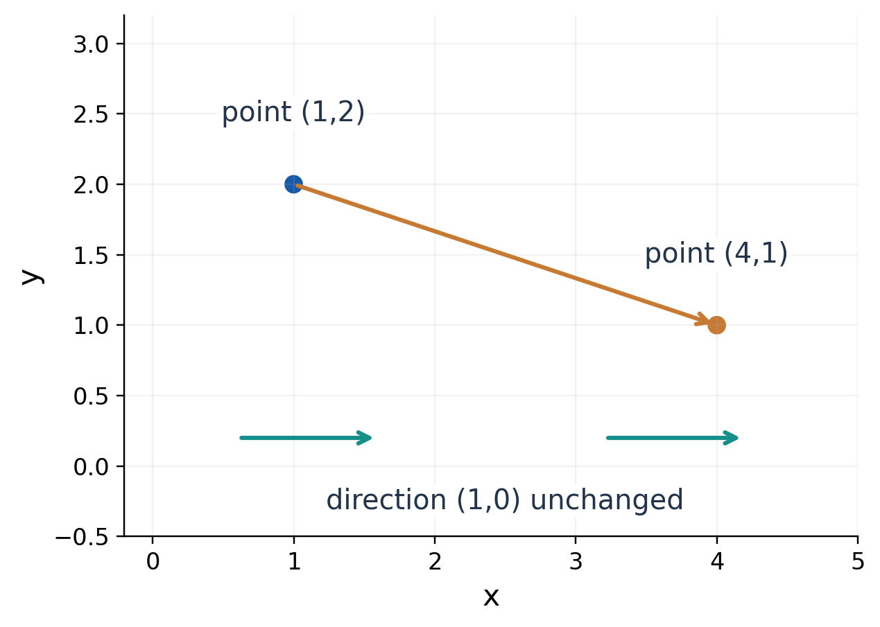
Worked Example 4.143 – Scale Then Translate
Embed S_h=diag(2,1,1). TS_h maps (1,2,1)ᵀ to (5,1,1)ᵀ. Reversing the order gives (8,1,1)ᵀ. Translation and scaling need not commute.
A 3D column-vector pipeline may write clip coordinates equal PVM times the local coordinate vector for model, view and projection matrices. The rightmost stage acts first.
Perspective conversion then divides by the homogeneous w-coordinate where w≠0. This separate division is nonlinear in the resulting Cartesian coordinates, even though the preceding homogeneous multiplication is linear.
Three-dimensional affine transformations commonly use 4×4 matrices with point columns (x,y,z,1)ᵀ. Some projection stages lose depth information and are not invertible.
Coordinate Check
Keep the homogeneous coordinate until the appropriate conversion. Directions have w=0 and cannot be treated as ordinary points for perspective division.
Worked Example 4.144 – Translate a Direction
Use the same T on the homogeneous direction d=(1,0,0)ᵀ:
Td = (1,0,0)ᵀ.
The translation terms multiply the final coordinate zero and vanish. Treating a direction as (1,0,1)ᵀ would instead turn it into a point and incorrectly add the translation. Points and directions must retain different homogeneous representations.

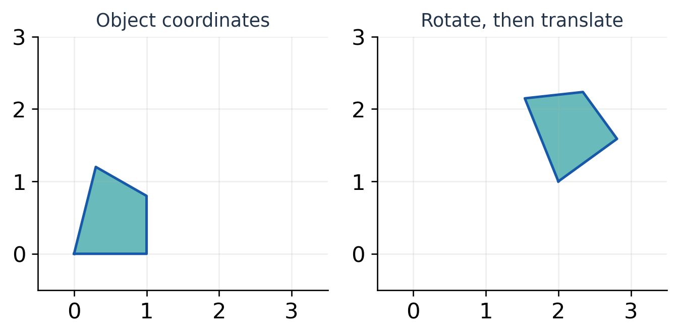
49. Loop-Current Analysis
Consider clockwise mesh currents I₁,I₂, exclusive resistances 3 Ω and 4 Ω, a shared 2 Ω resistor, and source rises 8 V and 2 V in the respective traversal directions.

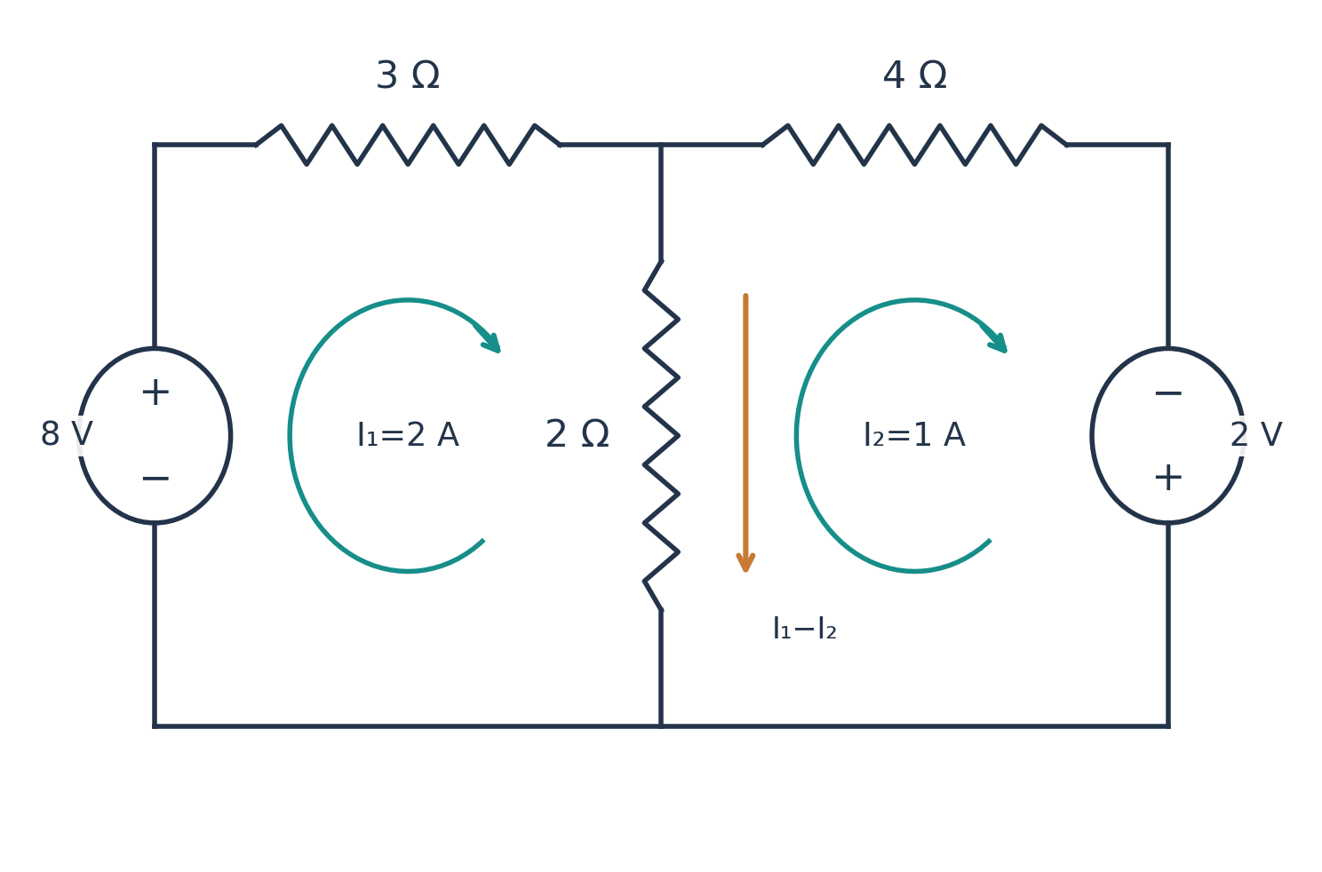
Kirchhoff’s equations are:
3I₁+2(I₁−I₂)=8.
4I₂+2(I₂−I₁)=2.
In matrix form:
[5,−2],[−2,6]ᵀ = (8,2)ᵀ.
The shared current is a difference because both clockwise traversals oppose along that branch.
Worked Example 4.145 – One Circuit Iteration
Gauss–Seidel from zero gives:
I₁^(1) = 8/5 = 1.6.
I₂^(1) = [2+2(1.6)]/6 = 0.866667…
The next sweep gives approximately (1.946667,0.982222), moving toward (2,1). This provides another check that direct and convergent iterative methods target the same physical equation system.
Worked Example 4.146 – Mesh Currents
Multiply the first equation by 3 and add the second, obtaining 13I₁=26. Thus I₁=2 A. Substitution gives I₂=1 A.
Checks: 10−2=8 and −4+6=2. The shared current is 1 A downward in mesh 1’s common-branch direction.
Worked Example 4.147 – Power Balance
P_R = 3(2)²+4(1)²+2(2−1)² = 18 W.
Source power supplied is 8(2)+2(1)=18 W. This independently checks current signs and source polarities.
The coefficient matrix is symmetric with leading minor 5>0 and determinant 26>0, so it is positive definite. It is also strictly diagonally dominant, making Gauss–Seidel suitable as well as direct elimination.
Circuit Sign
Adding the two mesh currents in this common resistor would contradict the selected directions. Write the branch direction before forming voltage drops.
Energy and the Coefficient Matrix
The resistor dissipation can also be written IᵀAI for this mesh matrix. At I=(2,1)ᵀ it equals Iᵀb=18 W.
Positive definiteness means IᵀAI>0 for every nonzero real current vector in this resistive model. The off-diagonal negative terms represent the shared-branch coupling; they do not imply negative resistor values.
50. PCA: Covariance and Eigenvectors
For n centred real observations stored as rows of X, sample covariance is:
C = XᵀX/(n−1).
It is symmetric and has nonnegative quadratic form. Orthogonal eigenvectors give principal directions, with eigenvalues equal to variances along them.
Worked Example 4.148 – Centre and Form Covariance
The data (−2,−2),(−1,−1),(1,1),(2,2) have mean zero:
X = [[−2,−2],[−1,−1],[1,1],[2,2]].
C = (1/3)[[10,10],[10,10]].

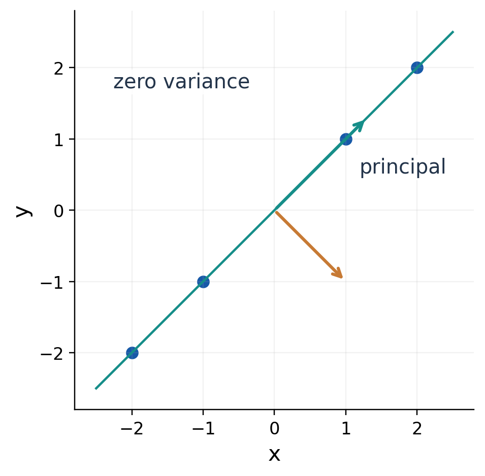
Compute and Interpret the Components
The eigenvalues are 20/3 and 0, with unit directions u₁=(1,1)ᵀ/√2 and u₂=(1,−1)ᵀ/√2.
Worked Example 4.149 – Project Observations
Xu₁ = (−2√2,−√2,√2,2√2)ᵀ.
Their sample variance is (8+2+2+8)/3=20/3. The second scores all vanish.
The total variance is trace C=20/3. Keeping one component retains 100% for this exact collinear dataset, not for arbitrary real data.
Subtract the mean before covariance calculations. Otherwise XᵀX describes variation about the origin rather than about the data mean.
Feature scaling also matters. Covariance PCA and correlation-matrix PCA represent different choices when units or feature magnitudes differ.
PCA Sequence
Centre, form the stated covariance, choose orthonormal eigenvectors in decreasing eigenvalue order, then project. State whether the divisor is n−1 or n.
Worked Example 4.150 – Translate All Observations
Add (10,10) to every observation. The new mean is (10,10), and subtracting it returns exactly the original centred X.
The covariance and principal directions therefore remain unchanged after consistent centring. Without centring, the large offset would contribute to XᵀX and could dominate the apparent direction of variation.

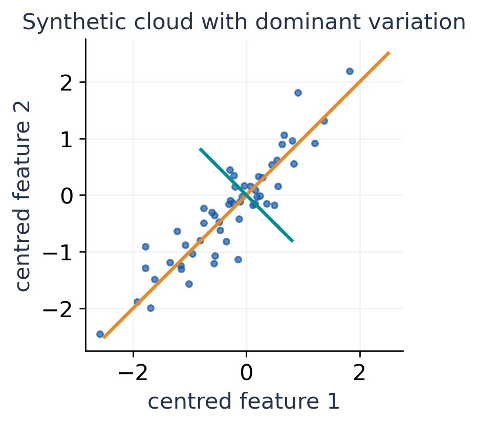
51. PCA Reconstruction
With orthonormal retained directions U_r, a centred x is multiplied by the transpose of U_r to obtain its scores; reconstruction uses:
x̂ = U_r U_rᵀx, e = x−x̂.
The residual is perpendicular to the retained directions. Add the mean back when reconstructing original coordinates.
Worked Example 4.151 – Exact Rank-One Data
For u₁=(1,1)ᵀ/√2 and x=(2,2)ᵀ, score 2√2 reconstructs (2,2)ᵀ exactly. The residual is zero.

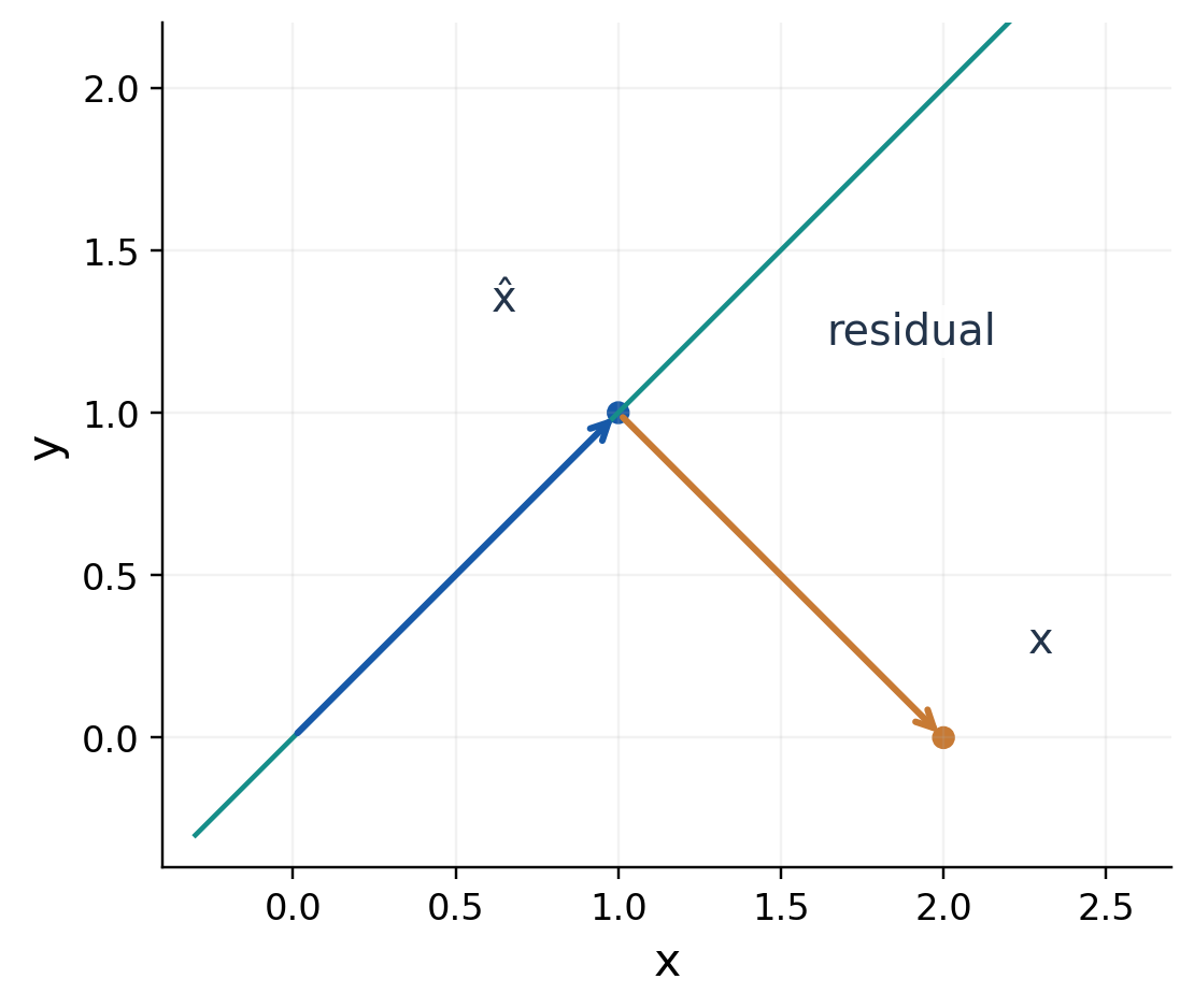
Worked Example 4.152 – Write the Projector
For the retained unit direction:
P = u₁u₁ᵀ = (1/2)[[1,1],[1,1]].
It satisfies P²=P and Pᵀ=P. Applying it twice changes nothing after the first projection. Its eigenvalues are 1 along the retained direction and 0 along the discarded direction, connecting projection, rank and eigenanalysis.
Worked Example 4.153 – Retain One Component
For the stated covariance C with rows (2,1),(1,2), eigenvalues are 3 and 1. Retaining the first direction keeps 3/4=75% of aggregate variance.
For x=(2,0)ᵀ:
z = √2, x̂ = (1,1)ᵀ, e = (1,−1)ᵀ.
The error magnitude is √2, and e·u₁=0. The 75% variance figure is a dataset-level property of the covariance, not a promise that every point retains exactly 75% of its squared length.
Compression stores fewer scores per observation after accounting for the shared mean and basis. Its usefulness depends on preserving information relevant to the task.
Projection Condition
The retained-direction projector is orthogonal only when the columns of U_r are orthonormal. A general nonorthonormal basis needs a different projection expression.
Worked Example 4.154 – Add the Mean Back
For mean (10,10) and original vector (12,10), the centred vector is (2,0). Its one-component reconstruction is (1,1).
Adding the mean gives reconstructed original coordinates (11,11), with residual (1,−1). Forgetting the mean at either end would compare or display vectors in different coordinate frames.
52. Face-Recognition Matrix Models
A classical eigenface-style pipeline aligns images, vectorises pixels, subtracts the reference mean and projects onto principal-component directions. Score vectors are compared with stored references.

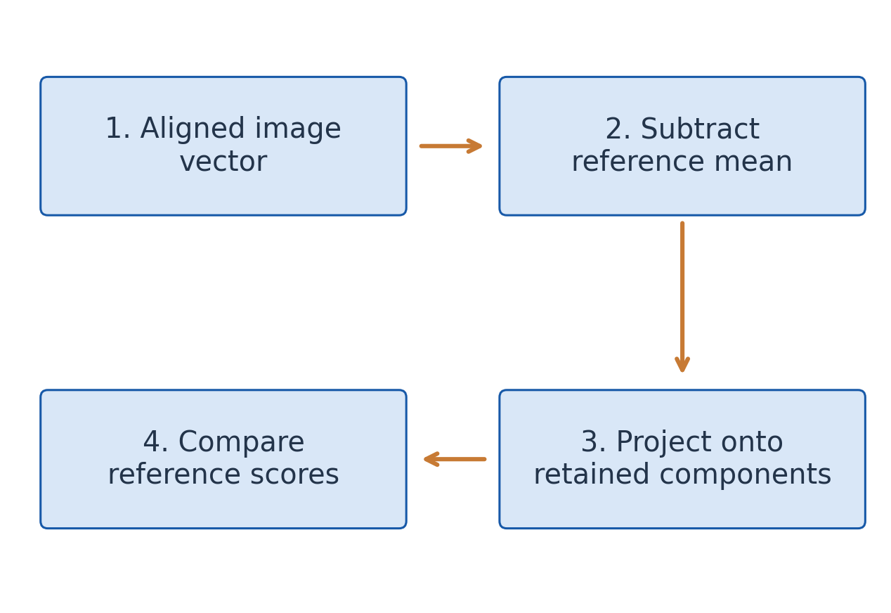
Covariance eigenvectors can be reshaped as image patterns. In high dimensions, an equivalent smaller eigenproblem or SVD is often used computationally, while retaining the same projection concept.
This describes one mathematical approach, not a complete recognition system or a claim of accuracy on real faces.
Dimensions of a Projection Pipeline
| Object | Dimensions |
|---|---|
| Centred data X | n×d |
| Retained directions | d×r |
| Score matrix | n×r |
| One score column | r×1 |
Rows of data are observations; columns are features. The shared component matrix maps each centred observation to fewer coordinates. Checking these shapes catches accidental transposes before distance calculations.
Worked Example 4.155 – Compare Compressed References
Let μ=(10,10)ᵀ, u=(1,1)ᵀ/√2, references A=(12,10)ᵀ,B=(8,8)ᵀ and query q=(11,11)ᵀ. After centring:
z_A = √2, z_B = −2√2, z_q = √2.
Distances in score space are 0 to A and 3√2 to B, so the toy rule selects reference A.
A and q are not identical original vectors. Their difference is perpendicular to u and has been discarded. Compression can remove useful distinctions along with unwanted variation.
References and queries need the same alignment, scale, mean and component basis. Scores using different preprocessing cannot be compared meaningfully.
Scope
These two-feature numbers illustrate projection and comparison, not real face pixels or real recognition performance. Correct matrix arithmetic does not establish a deployed system’s accuracy.
A Distance Can Disappear Under Compression
The original difference between A and q is (1,−1), with norm √2. Its projection onto u=(1,1)/√2 is zero.
Thus their equal compressed scores do not make the original features equal. A retained subspace preserves distances within it, but can remove distinctions perpendicular to it. This explains the limitation directly from the example’s arithmetic.

53. Mixed Solved Revision
Worked Example 4.156 – Rank and Inverse
For A with rows (1,2),(2,4), R₂−2R₁ produces a zero row. Rank is 1 and determinant 0, so no inverse exists.
Worked Example 4.157 – Complex Classification
H with rows (2,i),(−i,2) satisfies H†=H. Its eigenvalues 3,1 are real, confirming the expected spectral location.
Worked Example 4.158 – Solve by Elimination
From x+y=3 and 2x−y=3, addition gives 3x=6. Hence x=2,y=1.
Worked Example 4.159 – A Nonunit Eigenvector
For diag(4,−1), v=(0,2)ᵀ maps to (0,−2)ᵀ=−v. Its eigenvalue is −1; eigenvectors need not be unit length.
Worked Example 4.160 – A Quick Spectral Check
For diag(3,−2), trace is 1 and determinant is −6. The eigenvalues 3 and −2 have the same sum and product.
Because the matrix is diagonal, coordinate axes are eigenvectors immediately. This special ease does not extend to every nondiagonal matrix with the same diagonal entries.
Worked Example 4.161 – One Iterative Sweep
For 4x+y=6,x+3y=7, start at (1,1). Then x_new=5/4 and:
y_new = (7−5/4)/3 = 23/12.
Using old x=1 would instead give 2, a different update rule.
Worked Example 4.162 – Orthogonal Inverse
For 90° rotation R, R⁻¹=Rᵀ rotates back clockwise. The two successive actions return any vector to its original coordinates.
Worked Example 4.163 – Two Stability Models
The update x_(k+1)=−2x_k is unstable, whereas x′=−2x decays. Magnitude and real-part tests belong to different time models.
Worked Example 4.164 – Retained Variance
For covariance eigenvalues 9,3,0, keeping two gives 100% of total variance, while keeping only the first gives 75%.
Method Audit
Identify whether the task is reduction, iteration, eigenanalysis, coordinate change or projection before choosing a formula.
Worked Example 4.165 – Check the Revision Sweep
For the sweep (5/4,23/12), the residual is:
r = (−11/12,0)ᵀ.
The second equation is exact after its update, while the first is not. The improved components are still only an intermediate approximation. Checking both equations prevents reporting one sweep as a completed exact solve.
54. Short-Answer Checks
What Does Matrix Order Mean?
Rows followed by columns. An m×n matrix has m rows and n columns.
When Is AB Defined?
A’s column count equals B’s row count. The output has A’s row count and B’s column count.
Is A† Equal to Aᵀ?
For real matrices, yes. Complex adjoints also conjugate entries. Here † denotes conjugate transpose, not pseudoinverse.
What Is Rank by Echelon Form?
The number of pivots, equivalently the number of nonzero echelon rows.
Does Determinant Zero Mean No Solution?
No. A singular square matrix may give infinitely many solutions or none, depending on b.
Can a Rectangular Matrix Have an Ordinary Inverse?
An ordinary two-sided inverse of the type used here requires a square matrix. A rectangular full-column-rank matrix can have a left inverse, but that is a different statement and does not make both products identity of the same size.
Dimension checks should therefore precede any attempt to use the square inverse formula.
What Distinguishes Gauss–Seidel?
New components are reused immediately during a sweep. Convergence depends on the matrix and ordering, not just nonsingularity.
Why Exclude the Zero Eigenvector?
It satisfies Av=λv for every λ and therefore identifies no specific eigendirection or eigenvalue.
Do Repeated Roots Prevent Diagonalisation?
Not necessarily. Count independent eigenvectors and compare eigenspace dimensions with algebraic multiplicities.
Does Row Reduction Preserve Eigenvalues?
Generally no. Similarity preserves spectra; elementary row operations preserve rank and augmented-system solutions.
What Are the Stability Tests?
Discrete asymptotic stability uses |λ|<1; continuous asymptotic stability uses Re λ<0. Boundary cases require an eigenstructure check for bounded behaviour.
Answer Standard
State the definition with its size, field or convergence assumptions. A shortcut without conditions can give a wrong conclusion.
When Can Transpose Replace Inverse?
For a real orthogonal matrix, Q⁻¹=Qᵀ. For a complex unitary matrix, use U† instead. An arbitrary invertible matrix has neither shortcut.
Does a Small Residual Prove an Accurate Solution?
Not by itself. Scaling and conditioning can amplify solution error relative to the equation mismatch. State what was checked and the tolerance used.
55. Formula Sheet
Matrix and Adjoint Rules
(AB)ᵀ = BᵀAᵀ.
(AB)† = B†A†.
(AB)⁻¹ = B⁻¹A⁻¹.
H†=H, K†=−K, U†U=I.
Inverse products require invertible square factors. Adjoint reverses order and conjugates scalar entries.
For consistent n-variable systems, the number of free parameters is n−rank(A). Consistency requires equal coefficient and augmented ranks; uniqueness requires that common rank to be n.
Eigenproblem
Av=λv, v≠0, det(A−λI)=0.
Σᵢλᵢ=tr A, Πᵢλᵢ=det A.
Count algebraic multiplicity in the spectral sums and products.
Diagonalisation and Applications
A=SDS⁻¹, Aᵏ=SDᵏS⁻¹.
QᵀAQ=D for real symmetric A.
S needs n independent eigenvectors; Q uses an orthonormal eigenvector basis.
Gauss–Seidel
xᵢ^(k+1) = [bᵢ−Σ(j<i) aᵢⱼxⱼ^(k+1)−Σ(j>i) aᵢⱼxⱼ^(k)]/aᵢᵢ.
r = b−A x̃.
Nonzero diagonal entries are needed for this update. Strict diagonal dominance or real symmetric positive definiteness suffices for convergence; in general require ρ(T)<1.
PCA and Binary Checks
C = XᵀX/(n−1), z=U_rᵀx, x̂=U_rz.
s = Hr mod 2.
PCA assumes centred data and orthonormal retained directions. Coding requires modulo-2 arithmetic and a stated error model.
Final Audit
Check dimensions, pivots, original equations, residuals, eigenvector pairing, coordinate conventions and the correct time model before rounding the final answer.


