Course: Introduction to AI & Prompt Engineering | AKTU B.Tech First Year | Semester I & II
Course Codes: AAI101 / AAI201
Streams: CSE, EE, ECE, CE, ME, BT, CH, TX & AG
Unit IV Overview
These AI and Prompt Engineering Unit 4 Notes connect AI methods with engineering problems, measurements and decisions. Each application is explained through its problem, input data, model output, practical use, validation and limitations.
The unit covers structural monitoring, smart cities, traffic optimisation, predictive maintenance, design, robotics, smart grids, fault detection, VLSI, coding assistance, cybersecurity, language interfaces, biotechnology, healthcare, agriculture, chemical processes, textiles and material design.
It also examines bias, privacy, workforce changes and responsible oversight.
The emphasis is conceptual. A useful answer identifies the computation and evidence rather than merely naming a branch or saying that AI improves efficiency.
Small numerical examples are synthetic unless explicitly identified as a reported historical case.
Topics Covered
| Topic | Source PDF Pages |
|---|---|
| Application workflow and validation | 2 |
| CE: structural monitoring, smart cities and traffic | 3–5 |
| ME: maintenance, design and robotics | 6–8 |
| EE / ECE: grids, faults and VLSI | 9–11 |
| CSE: code, cybersecurity and language interfaces | 12–14 |
| BT / healthcare: discovery research and imaging | 15–16 |
| Genomics and wearables | 17 |
| AG: precision farming, crop monitoring, aerial sensing and soil | 18–20 |
| CH: process optimisation | 21 |
| TX: textile quality control | 22 |
| Material design | 23 |
| Bias, privacy and job displacement | 24–26 |
| Real case and group presentation activity | 27 |
| Revision and examination practice | 28 |
Learning Outcomes
- Explain structural monitoring, smart-city services and traffic tasks.
- Describe predictive maintenance, constrained design and robot perception / control.
- Identify forecasting, fault-detection and chip-design outputs.
- Explain code assistance, defensive cybersecurity and natural-language interfaces.
- Distinguish research predictions from experimentally or clinically established outcomes.
- Describe agricultural sensing, spatial variation and targeted decisions.
- Connect process measurements, textile inspection and material properties to appropriate model outputs.
- Assess bias, privacy, workforce effects and responsible oversight.
- Present a real application as problem → data → AI solution → impact, with a meaningful limitation.
Included in These Notes
Detailed explanations across all nine engineering streams, comparison tables, 25 numbered diagrams and illustrations, worked numerical checks, constrained-selection exercises, historical application examples, a two-minute group presentation plan, complete exam-answer explanations and quick revision.
The 25 extracted PNG files follow the article’s Img numbering.
Conceptual robot, DNA and aerial-sensing illustrations are included along with vector diagrams and application workflows.
Study Approach
Name the problem. Specify the engineering need before selecting a model.
Identify available data. Record measurements, units, collection conditions and prediction time.
State the output. Distinguish a category, numerical estimate, region, candidate design, explanation or actuator command.
Connect output to action. Identify who reviews the result and which constraints govern the decision.
Evaluate the workflow. Compare a meaningful baseline, inspect relevant errors and state operating limitations.
Stream and Course Coverage
| Applicable Streams | Semester I Code | Semester II Code | Unit |
|---|---|---|---|
| CSE, EE, ECE, CE, ME, BT, CH, TX and AG | AAI101 | AAI201 | Unit IV: AI Applications Across Engineering Domains |
These AI and Prompt Engineering Unit 4 Notes follow the common unit coverage in the supplied PDF.
Read other domains as applications of shared input–model–output principles. Additional study resources are available at www.notesgallery.com.
Essential Vocabulary
| Term | Meaning |
|---|---|
| Monitoring | Observe condition over time |
| Forecast | Estimate a future quantity |
| Anomaly | Deviation from an expected pattern |
| Optimisation | Choose a candidate under objectives and constraints |
| Decision support | Information used by a responsible decision-maker |
| Deployment | Use in actual operating conditions |
| Validation | Check the intended claim against appropriate references |
| Distribution shift | A change between development and later operating conditions |
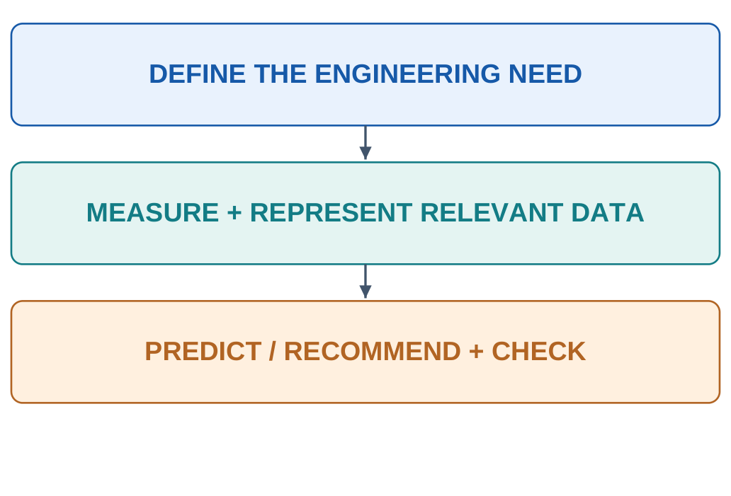
4.1 From an Engineering Problem to an AI Task
An engineering application begins with an operational problem.
A bridge may need inspection, a machine may develop an unusual vibration pattern or a field may have uneven water availability.
Translate that problem into a specific task before selecting a model.
The task might be classification, numerical prediction, anomaly detection, optimisation or content generation.
Each requires different reference information and evaluation.
A category score and an actuator command are not interchangeable outputs.

| Need | Possible AI Task |
|---|---|
| Find likely defects | Classification / detection |
| Estimate tomorrow’s load | Forecasting |
| Identify unusual operation | Anomaly detection |
| Choose a lighter candidate | Constrained optimisation |
| Draft an explanation | Language generation |
4.1.1 A Complete Application Description
A complete answer should identify:
- Problem: What practical difficulty is being addressed?
- Data: What is measured and when is it available?
- Output: Category, number, location, candidate or text?
- Action: Who uses it and what decision follows?
- Validation: What reference and conditions test usefulness?
For a maintenance predictor, useful inputs may include past vibration and temperature readings.
If the intended prediction is made before a failure, future repair notes must not appear as input. Otherwise the evaluation can leak the answer.
Choose a baseline such as a fixed inspection schedule or a simple forecasting rule.
Comparing only with doing nothing can overstate the benefit of a complex model.
Evaluate the whole workflow, including false alarms and staff effort.
4.1.2 Development and Deployment Differ
A model fitted on one machine, hospital, fabric or crop may encounter different measurements later.
This change is often called distribution shift.
The physical operating environment matters as much as the model’s name.
Deployment also needs monitoring, clear responsibility and a way to handle unsupported cases.
A visually polished dashboard is not evidence that the underlying model remains valid.
Reusable answer frame
“Using [data], a model produces [output] to support [decision]. It is checked against [reference] under [conditions]. A major limitation is [specific failure].”
Fill every part with concrete information.
4.2 CE: Structural Health Monitoring
Structural Health Monitoring (SHM) collects and interprets information about a structure’s condition over time.
AI can help identify patterns that differ from a suitable baseline, prioritise inspection or estimate a defined condition-related quantity.
Possible inputs include vibration, strain, displacement, temperature and images.
These measurements describe different aspects of behaviour.
A temperature-induced change in response should not automatically be labelled structural damage.

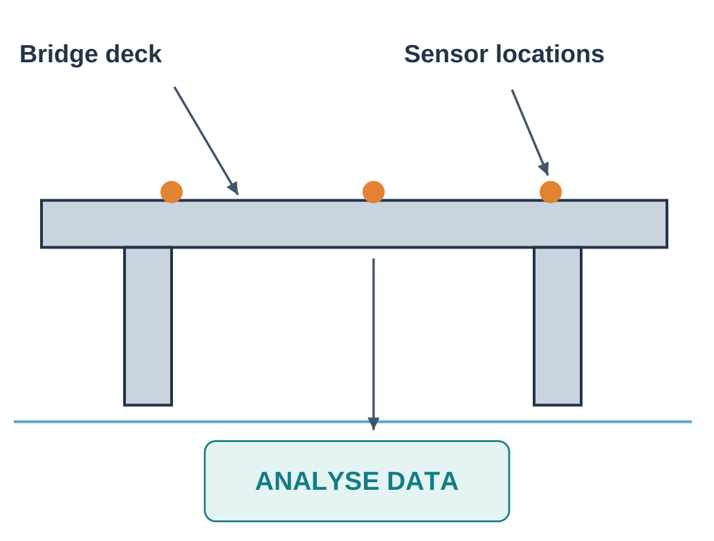
4.2.1 A Conceptual Workflow
Step 1: Establish suitable baseline observations.
Step 2: Collect time-stamped measurements consistently.
Step 3: Prepare features and check sensor quality.
Step 4: Compare current behaviour with an expected pattern.
Step 5: Investigate flagged cases using appropriate inspection.
4.2.2 Inputs, Outputs and Decisions
| Input | Possible Model Output |
|---|---|
| Vibration histories | Unusual-response flag |
| Labelled crack images | Candidate crack location |
| Strain and environmental records | Expected response estimate |
| Repeated inspections | Prioritisation information |
An anomaly flag indicates a deviation under the model, not a complete diagnosis of structural safety.
Investigate physical causes, sensor faults and changed operating conditions.
Decisions about a structure require qualified engineering assessment.
Image-based crack detection can mark a visible surface feature.
It cannot establish hidden reinforcement condition or a complete load-bearing assessment from that photograph alone.
4.2.3 A Small Illustrative Case
Suppose the usual measured response differs between cool mornings and hot afternoons.
A model trained only on morning data flags many afternoon readings.
The pattern may describe environmental variation rather than a new defect.
Include relevant conditions in development and evaluation.
Test on separate time periods and assets where appropriate.
Near-duplicate images of the same crack should not make a test appear independent when it is not.
Evaluation focus
Inspect missed concerning cases, unnecessary alarms and performance under relevant temperature, load and sensor conditions.
Overall accuracy alone may hide errors important to inspection planning.
4.3 CE: Smart Cities
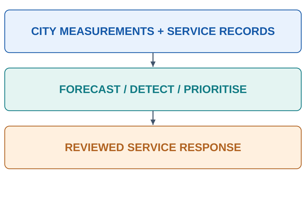
A smart-city application uses information and computation to support urban services.
AI may forecast demand, identify infrastructure faults or recommend resource allocation.
A city is not made intelligent merely by adding cameras or calling a dashboard AI.
Examples include estimating waste-collection demand, detecting water-network anomalies and forecasting traffic or energy patterns.
The outputs support specific service decisions and should be assessed against those decisions.

| Service | Illustrative Task |
|---|---|
| Water supply | Identify unusual consumption / flow patterns |
| Waste collection | Estimate pickup demand |
| Street infrastructure | Prioritise reported defects |
| Transport | Forecast congestion / travel conditions |
4.3.1 Data Integration
A city may combine sensor measurements, geographic information and service reports.
The records need compatible locations, times and definitions.
If two departments use different area codes, merging them carelessly can create false patterns.
Missing complaints do not necessarily mean a neighbourhood has no service problem.
Some residents may have less access to a reporting app.
Training only on app submissions can reproduce an unequal picture of need.
4.3.2 Decisions Have Multiple Objectives
A model that minimises average waiting time may still leave one neighbourhood poorly served.
Include relevant service constraints, accessibility and the distribution of outcomes rather than evaluating only one average.
A useful system should allow staff to inspect evidence and correct a misleading recommendation.
Human review is meaningful only if reviewers have time, information and authority to act.
| Question | Why It Matters |
|---|---|
| Whose observations are missing? | Coverage can be unequal |
| What is being optimised? | Objectives shape recommendations |
| Are locations and times aligned? | Incorrect joins create misleading inputs |
| Who can contest an outcome? | Errors need a correction route |
Sensors gather measurements, AI estimates patterns or proposes actions, and municipal processes decide and implement changes.
Describe these responsibilities separately.
4.4 Traffic Optimisation
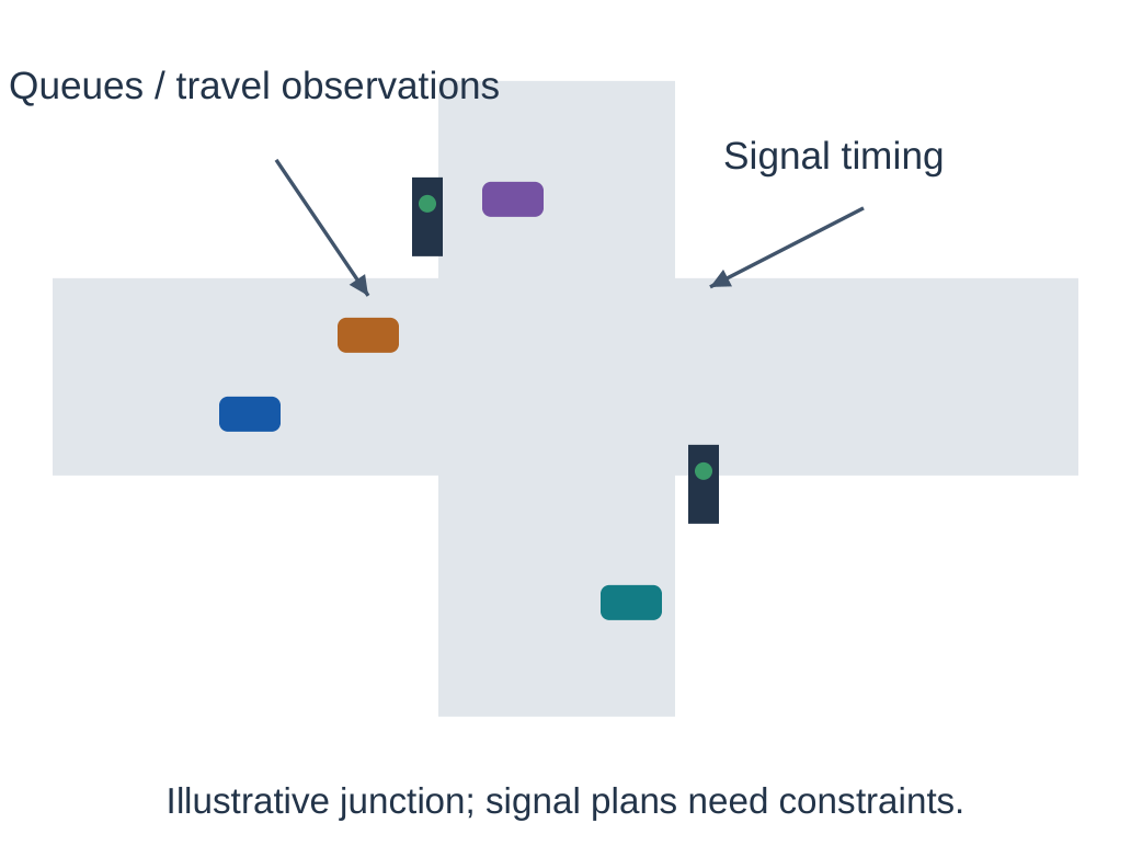
Traffic optimisation aims to improve movement subject to constraints such as pedestrian crossings, road capacity and emergency needs.
AI can estimate flow, forecast queues and support changes to signal timing.
Optimising one intersection can affect neighbouring intersections.
Inputs may include traffic counts, travel-time patterns and permitted sensor observations.
Outputs can be queue estimates or timing recommendations.
A proposed timing plan must still respect the traffic authority’s operational constraints.

4.4.1 What Should Be Evaluated?
- Delay and queue patterns under comparable demand.
- Effects on pedestrians and different travel directions.
- Performance during unusual events and sensor gaps.
- Whether improvements persist beyond a short trial.
- Changes at nearby junctions, not only one location.
4.4.2 Real Example: Project Green Light
The supplied notes discuss Google Research’s Project Green Light as an example of using driving trends and AI to model traffic patterns and recommend signal-timing changes to city traffic engineers.
The conceptual lesson is recommendation support.
It should not be described as an unrestricted chatbot directly controlling traffic lights.
Observed travel patterns inform timing proposals, while local engineers and operational constraints remain part of the workflow.
Benefits depend on location and evaluation conditions.
Do not copy one reported result as a universal improvement rate.
4.4.3 A Synthetic Comparison
| Trial | Mean Observed Delay |
|---|---|
| Baseline period | 50 seconds |
| Comparable trial period | 40 seconds |
| Difference | 10 seconds lower |
| Relative reduction | 10/50 = 20% |
Step 1: Calculate the difference
50 − 40 = 10 seconds
Step 2: Calculate relative reduction
(10/50) × 100 = 20%
The table is invented for arithmetic practice.
A 20% reduction follows from the supplied means.
It does not prove that AI caused the change. Demand, weather, incidents or measurement conditions could also differ.
A stronger evaluation accounts for relevant conditions, reports the observation period and checks other road users.
4.5 ME: Predictive Maintenance
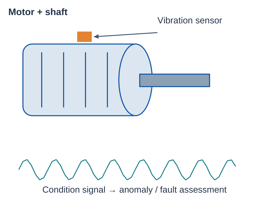
Predictive maintenance uses condition and historical information to estimate maintenance needs before a defined failure or unacceptable operating state.
It differs from repairing only after failure and from servicing solely at fixed time intervals.
Possible inputs include vibration, temperature, current, operating load and maintenance records.
Models can flag anomalies, classify a known fault pattern or estimate a quantity related to future condition.
These are related but distinct tasks.

| Approach | Maintenance Trigger |
|---|---|
| Reactive | Failure or breakdown |
| Preventive | Planned interval / usage rule |
| Predictive | Condition-based estimate under a defined process |
4.5.1 From Signal to a Work Order
First check the sensor, operating context and data quality.
Transform the signal into a suitable representation or use a model designed for it.
The prediction can then be reviewed alongside maintenance history before an action is planned.
A rising vibration feature might reflect a bearing issue, a different operating load or a mounting change.
The output should support investigation rather than replace the relevant mechanical diagnosis.
4.5.2 Labels and Lead Time
A useful prediction needs a defined horizon.
For example, the target might be the risk of a specified event within a future operating period.
An alarm produced after the event does not demonstrate useful advance prediction.
Failure records can be rare and uneven.
Repeated samples from one machine must be handled carefully when splitting development and test data.
Otherwise a model may recognise the machine rather than generalise to a new asset.
| Error / Issue | Practical Effect |
|---|---|
| False alarm | Unnecessary inspection or downtime |
| Missed event | Maintenance opportunity lost |
| Late warning | Little useful preparation time |
| Changed operating regime | Past patterns may no longer apply |
The source notes use Siemens maintenance systems as a real-world connection.
The general lesson is to link relevant measurements to a maintenance workflow, rather than assume that every unusual signal has one fixed cause.
A remaining-useful-life estimate is a numerical target under defined conditions, not a guaranteed failure date.
4.6 ME: Design Optimisation
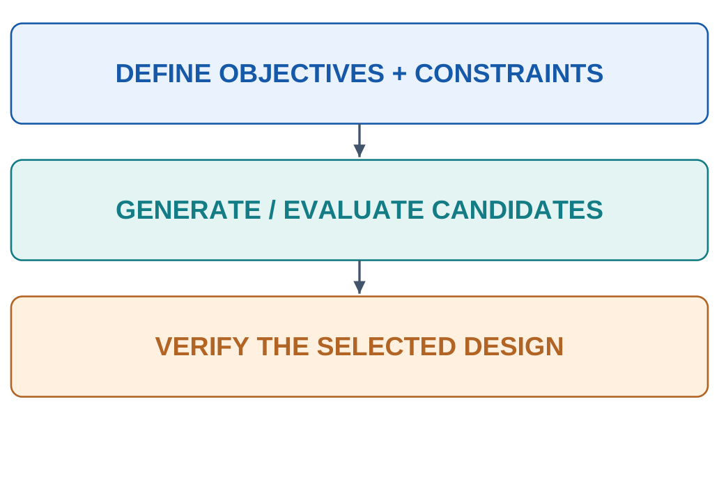
Design optimisation searches for a candidate that meets objectives while satisfying constraints.
A model may approximate performance, rank designs or help explore a large set of alternatives.
Engineering checks still determine whether a candidate is acceptable.
For a bracket, objectives might include lower mass or manufacturing cost.
Constraints can include load, deformation, permitted material and manufacturing requirements.
Without constraints, “make it lighter” is an incomplete design problem.

| Element | Illustrative Bracket Problem |
|---|---|
| Design variables | Permitted geometry dimensions |
| Objective | Reduce mass |
| Constraints | Required strength and stiffness |
| Evaluation | Suitable analysis and validation |
| Decision | Choose a feasible candidate |
4.6.1 A Synthetic Candidate Table
| Candidate | Mass | Constraint Check |
|---|---|---|
| A | 1.0 kg | Pass |
| B | 0.8 kg | Fail |
| C | 0.9 kg | Pass |
Among these three candidates, C is the lowest-mass feasible option.
B is lighter but fails the required check. It cannot win a constrained comparison solely on mass.
The table is a teaching example, not a tested component design.
If cost, manufacturability and durability also matter, objectives may conflict.
A set of trade-off candidates can be more informative than pretending that every goal has one universal maximum.
4.6.2 Generative Design Versus GenAI Text
Generative design explores candidate designs under objectives and constraints.
A chatbot that describes a lightweight part has not necessarily performed that optimisation.
A visually plausible shape is not equivalent to an analysed feasible component.
The supplied notes use Autodesk and Airbus’s bionic-partition work as a design-exploration example.
It illustrates an engineering workflow involving constraints and manufacturing research, rather than a text-to-image tool validating aircraft hardware.
A learned surrogate can be inaccurate outside the region it represents.
Check selected candidates using appropriate independent engineering methods and relevant manufacturing conditions.
4.7 ME: Robotics
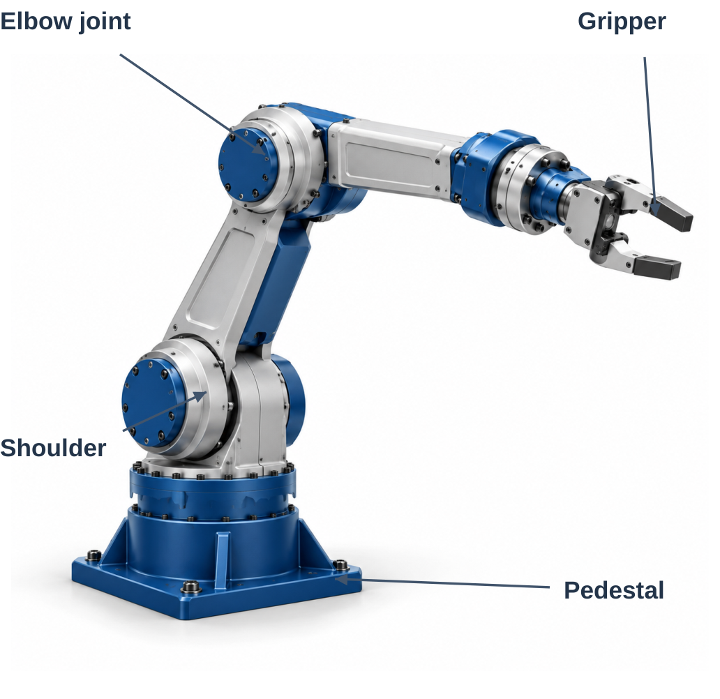
Robotics combines sensing, decision-making and physical action.
AI can support object recognition, grasp selection, motion planning or learning a policy in a suitable environment.
A robot also depends on mechanical design, actuators, fixed control logic and operating constraints.
A camera-based model may estimate an object’s category and position.
Planning selects a permitted movement.
A controller coordinates actuator behaviour.
Calling the whole chain image recognition hides the differences between perception and action.

4.7.1 Perception–Planning–Action
Step 1: Observe the object and relevant workspace.
Step 2: Estimate the information needed for the task.
Step 3: Plan a movement within constraints.
Step 4: Execute through a suitable control system.
Step 5: Monitor feedback and handle deviations.
4.7.2 A Sorting Example
For a robot sorting parts, images may support category recognition while depth or other observations support location.
The model’s category score is not itself a motor command.
Planning and control convert the task into a permitted movement.
If two parts overlap, an uncertain visual estimate can produce a poor grasp target.
A good workflow identifies unsupported observations and requests another view or a suitable fallback.
| Stage | Possible Failure |
|---|---|
| Perception | Object missed because of occlusion |
| Planning | No feasible motion through available space |
| Control | Actual motion differs from intended motion |
| Task monitoring | A failed grasp is not detected |
4.7.3 Learning in Simulation
Simulation can provide controlled practice environments for some robot-learning methods.
The real world may differ in friction, lighting, contact or sensor noise.
This simulation-to-reality gap needs evaluation.
Not every robot learns by reinforcement learning.
Some combine supervised perception with conventional planning and control.
Identify the learning component and its feedback instead of assigning one method to every robot.
4.8 EE: Smart Grids and Forecasting
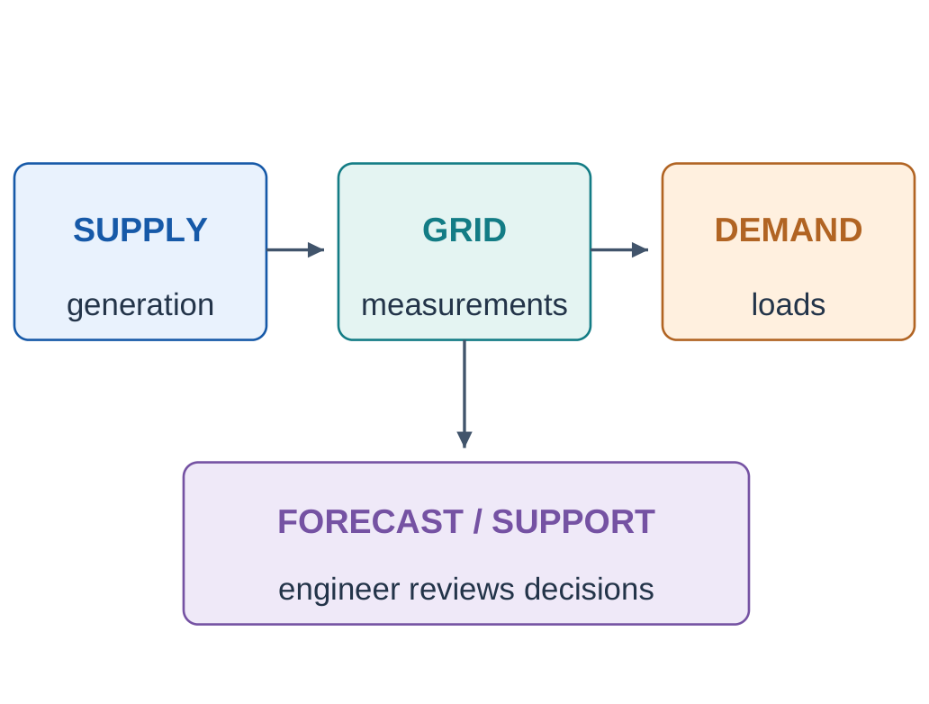
A smart-grid application uses measurements and communication to support electrical-network operation.
AI can forecast demand or renewable generation, detect abnormal patterns and assist planning.
Physical network limits and operational responsibility remain essential.
Demand forecasting predicts a future load value using relevant history and information available at prediction time.
Weather and calendar patterns can help, but unexpected events or changed consumption behaviour can reduce accuracy.

4.8.1 Tasks and Outputs
| Task | Output |
|---|---|
| Load forecasting | Future power-demand estimate |
| Renewable forecasting | Expected available generation |
| Anomaly screening | Flag for investigation |
| Planning support | Candidate allocation / schedule |
4.8.2 A Forecasting Example
Suppose a model predicts 120 units of demand and the observed value is 125 in the same stated unit.
Absolute error
|125 − 120| = 5 units
This is a numerical prediction task, so MAE can be relevant across several forecasts.
Use observations from the same intended horizon and preserve time order in evaluation.
Randomly mixing future information into training can give a misleading estimate of forecast quality.
4.8.3 Why a Forecast Is Not a Control Rule
A demand estimate supports scheduling, but a complete decision also needs operating limits, reserve requirements and other constraints.
A model cannot override those constraints merely because its forecast has low average error.
Uncertainty can matter as much as the central estimate.
A narrow-looking numerical output should not be interpreted as certainty about future load.
| Development Check | Reason |
|---|---|
| Use only available-time inputs | Avoid future-information leakage |
| Test different seasons / conditions | Check relevant variation |
| Compare a simple baseline | Establish useful added value |
| Inspect large errors | Averages can hide difficult periods |
Smart grid is an application context, not one neural-network architecture.
State the actual task and output before discussing a possible model.
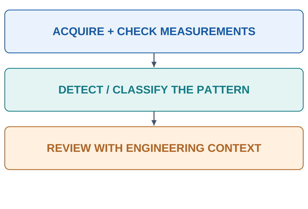
4.9 EE / ECE: Fault Detection
Fault detection identifies evidence of a defined abnormal condition.
Fault classification assigns a category.
Localisation estimates where the problem is.
Anomaly detection may flag an unusual pattern without knowing its precise cause.
Possible inputs include current and voltage-related measurements, temperature or device logs.
The representation must suit operating conditions and the measurement system.
A missing sensor value should not silently be treated as a normal reading.

| Question | Task |
|---|---|
| Is this pattern abnormal? | Detection |
| Which known fault class fits? | Classification |
| Where might it be located? | Localisation |
| What caused the event? | Further diagnostic reasoning |
4.9.1 False Alarms and Missed Cases
Define the positive class before using precision and recall.
If positive means a fault case:
Precision describes how many generated fault flags are correct.
Recall describes how many actual fault cases were flagged.
High overall accuracy can hide poor recall when normal operation dominates the test data.
Evaluate relevant fault types and operating regimes, not only the most frequent condition.
4.9.2 Synthetic Count Example
| Count | Value |
|---|---|
| Actual fault cases | 20 |
| Correctly flagged faults | 16 |
| Missed faults | 4 |
| Normal cases incorrectly flagged | 8 |
| Recall | 16/20 = 80% |
| Precision | 16/(16+8) ≈ 66.7% |
Recall calculation
Recall = TP / (TP + FN)
Recall = 16/(16 + 4) = 80%
Precision calculation
Precision = TP / (TP + FP)
Precision = 16/(16 + 8) ≈ 66.7%
The model finds most actual faults in this example, but one-third of its positive flags are false.
Report both conclusions.
An AI screening model is not a substitute for a validated protection function.
Changing load, sensor calibration or equipment type can alter the observed patterns.
4.10 ECE: VLSI Design Automation
Very Large Scale Integration (VLSI) design involves interacting choices about circuit structure and physical implementation.
AI can assist search, estimation and optimisation within design automation.
It does not remove the need for functional and physical verification.
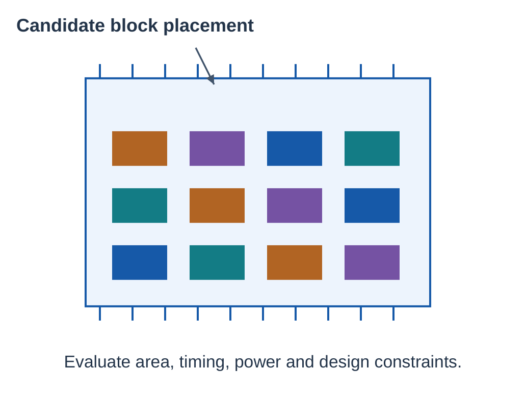
A placement task chooses where circuit blocks should be arranged on a chip area.
Connectivity and physical constraints influence the quality of a candidate layout.
Prediction can also help estimate timing, power or congestion-related outcomes.

| Quantity / Concern | Why It Matters |
|---|---|
| Area | Space available / consumed |
| Timing | Whether required signal timing is met |
| Power | Operating and thermal considerations |
| Routing / congestion | Whether connections can be implemented |
| Design rules | Physical feasibility constraints |
4.10.1 Prediction and Search
A learned estimator can score candidate layouts more quickly than a full expensive evaluation in some workflows.
Search explores candidates, while final verification checks the selected design.
An inaccurate estimator can favour a candidate that later fails.
Some research approaches formulate placement as sequential decisions and learn a policy with a reward tied to layout quality.
This is one use of reinforcement learning. Other design tasks can use different methods.
4.10.2 A Documented Research Example
The source notes discuss Google’s chip-placement research, later described under the AlphaChip name, as a reinforcement-learning example for macro-placement tasks.
It illustrates AI inside a specific design-automation stage.
It should not be described as a model independently completing every stage of an entire processor.
Reported results for a particular task or benchmark should not be generalized to every chip or design-flow stage.
4.10.3 Verification Remains Separate
A good predicted timing value does not prove logical correctness.
A physically compact layout does not guarantee acceptable power behaviour.
Several types of evidence are needed because the design has several requirements.
For an exam, connect netlist or block information to a placement or estimation output, explain the check and mention relevant constraints.
A colourful chip picture is an illustration.
A verified layout must meet connectivity, functional and physical requirements.
4.11 CSE: Code Generation and Assistance
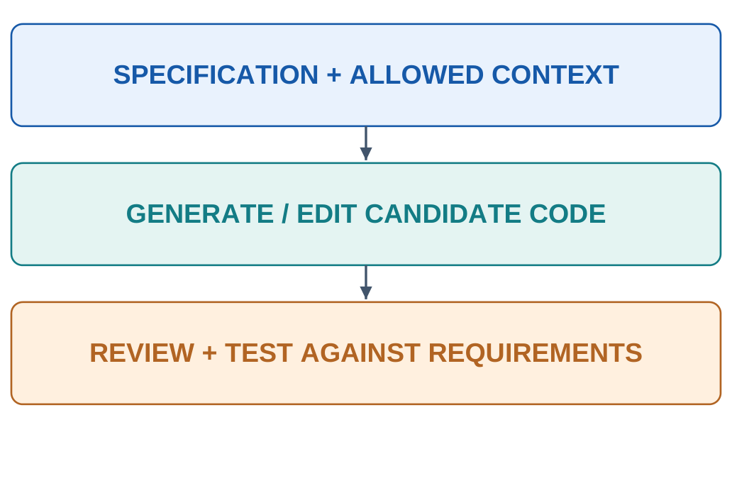
AI coding assistance generates or transforms candidate program text using instructions and available context.
GitHub Copilot is a syllabus example of assistance within software-development workflows.
It can support drafting code, explanations and related tasks depending on enabled features.
A generated program must still satisfy its specification.
Syntax, functional correctness, input handling and security are different checks.
An answer that compiles can still calculate the wrong result or make incorrect assumptions.

4.11.1 A Precise Specification
Teaching task
Read a list of numerical temperatures and return their mean.
Define what should happen for an empty list.
Do not assume all text inputs are already valid numbers.
The empty-list rule changes implementation and testing.
Without that rule, a model may invent a behaviour or divide by zero.
The specification should define the intended result before the code is accepted.
4.11.2 Review and Test
| Case | What It Checks |
|---|---|
| Two values 20 and 30 | Mean is 25 |
| One value 18 | Mean is 18 |
| Empty list | Stated error / empty policy |
| Malformed input | Defined validation behaviour |
| Large or unusual values | Relevant numeric handling |
These cases check meaningful behaviours rather than whether the code resembles an expected template.
The student should explain why a result follows from the specification.
Suggestions can contain insecure patterns, incorrect libraries or unsupported assumptions.
A model-produced explanation is not a replacement for reading the actual code.
4.11.3 Data and Project Context
Use only permitted source material.
Secrets and confidential code should not be copied into an unsuitable tool.
A repository-aware assistant may use files supplied by its application.
Do not assume it has read every dependency unless that context is actually available.
A suggestion matching an existing code pattern may raise attribution or licence considerations.
Follow project requirements and review relevant source-reference information.
Generated tests are also candidates.
They can repeat the same mistaken assumption as generated implementation.
Independently justify important expected results.
4.12 CSE: Cybersecurity Applications
AI can support defensive cybersecurity by identifying suspicious patterns, classifying messages or prioritising alerts.
Inputs may include permitted network summaries, event logs or labelled phishing examples.
The output should support an authorised defensive workflow.
A suspicious-pattern flag is not proof of an attack or a reliable identification of the person responsible.
Unusual activity can arise from legitimate changes.
Some malicious activity may resemble normal operation.

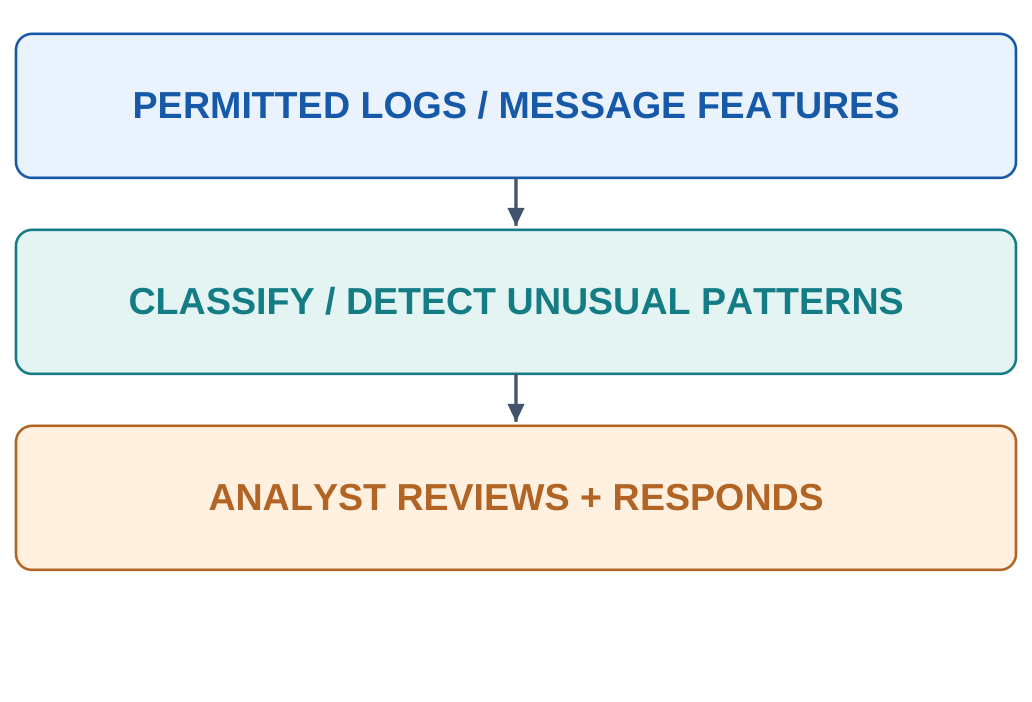
| Application | Possible Output |
|---|---|
| Phishing screening | Message category / risk flag |
| Network anomaly detection | Unusual activity alert |
| Malware-family classification | Known category estimate |
| Alert triage | Priority suggestions |
4.12.1 Labels and Changing Threats
Historical labels can be incomplete.
An incident may not have been discovered at collection time.
A model treating every uninvestigated record as safe can learn from misleading feedback.
Attack patterns, applications and normal business behaviour change.
Evaluate performance over relevant periods and inspect false alarms.
A detector that overwhelms analysts with routine activity may be ineffective despite a high headline score.
4.12.2 A Phishing Example
A classifier can use message-content features and other permitted indicators to flag a message for review.
The word urgent alone does not establish phishing.
Legitimate notices can be urgent, and harmful messages can avoid obvious keywords.
Do not evaluate only on repeated copies of the same message template across training and test groups.
That can reward template memorization rather than detection of new examples.
| Concern | Evaluation Response |
|---|---|
| Too many false alerts | Measure positive-flag quality |
| Rare harmful cases missed | Inspect recall on relevant cases |
| New patterns | Time-aware testing and monitoring |
| Sensitive log contents | Appropriate access and data handling |
A model should not trigger unrelated actions solely because it produced a high risk score.
Keep event detection, investigation and attribution distinct.
4.13 CSE: Natural-Language Interfaces
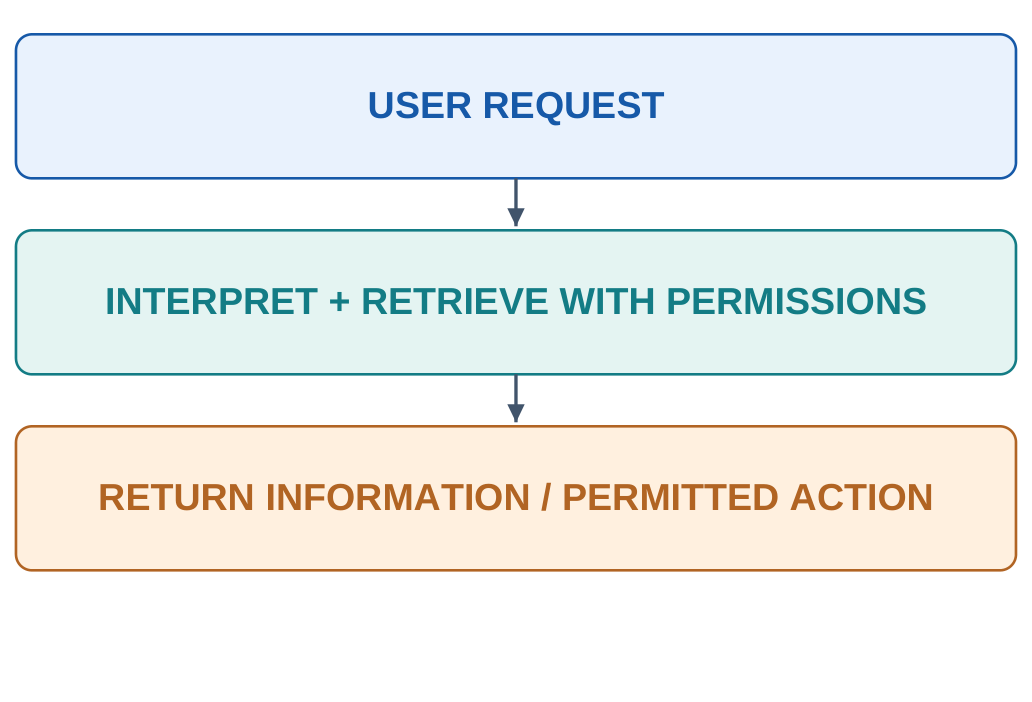
A natural-language interface allows a user to request information or actions using ordinary language.
The system must interpret the request, connect it to permitted application functions and produce a useful response.
An interface can combine speech recognition, language modelling, retrieval and fixed business rules.
Fluent conversation alone does not establish correct access, retrieval or execution.

4.13.1 A Campus-Notes Example
“Show Unit II notes for Introduction to AI and Prompt Engineering” names a subject and unit.
The interface must resolve the course correctly and retrieve the right item.
A similarly named document from another semester is not a successful match.
If the requested subject or unit is ambiguous, resolve that ambiguity rather than return a confidently worded guess.
4.13.2 Language Uncertainty and Application Rules
| Request Feature | What the System Needs |
|---|---|
| Tomorrow | A reference date and local context |
| My result | Correct identity and access permissions |
| Send the report | Resolved recipient and authorised action |
| These notes | The actual referenced file |
| Latest version | Current applicable document identity |
A model can propose an interpretation, while the application enforces who may access a record or perform an action.
Generated text must not bypass those checks.
A student asking politely for another person’s private result does not create permission.
For retrieval tasks, display the source clearly enough that the user can check the match.
For actions, ensure that the resolved input and actual operation correspond to the intended target.
4.13.3 Grounding and Failure Analysis
A response can fail because:
- The request was misinterpreted.
- The wrong document was retrieved.
- The final summary changed the evidence.
- The operation used the wrong target.
Check these stages separately.
Improving final wording does not repair retrieval of the wrong file.
When an answer is unavailable, an explicit gap is more useful than an invented record.
4.14 BT: Drug-Discovery Research
Drug discovery investigates candidate substances and their biological effects.
AI can support selected stages such as estimating molecular properties, prioritising candidates or analysing biological information.
A prediction helps decide what to investigate.
It does not establish that a substance is an effective or approved medicine.
Inputs may include molecular representations, experimental measurements or target-related information.
Outputs can be predicted properties or rankings.
The target and reference measurements must be defined before interpreting a score.

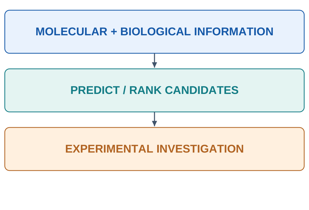
| Research Task | Possible Output |
|---|---|
| Property estimation | Predicted numerical property |
| Candidate screening | Ranked shortlist |
| Interaction modelling | Estimated compatibility |
| Information analysis | Patterns for investigation |
4.14.1 Prediction Versus Validation
A candidate with a high predicted interaction score may fail an experiment or have unsuitable properties elsewhere.
Selecting only for one objective can overlook other characteristics.
Training collections can be biased toward molecules that were already studied.
Predictions for a different chemical family may have less support.
Splitting nearly identical molecules across training and test groups can make generalization look easier than it is.
4.14.2 Protein-Structure Connection
AlphaFold is a documented example of learned protein-structure prediction discussed in the source notes.
Structural estimates can support biological research and help frame further questions.
A predicted structure does not by itself show the full behaviour of a protein or establish a drug’s effect.
Confidence can vary across a predicted structure.
A static representation may not capture every conformation, interaction or relevant experimental condition.
4.14.3 A Sound Application Answer
- Specify the biological research problem.
- Name the type of input representation.
- Identify the predicted property or candidate output.
- Describe the experimental check required.
- State a concrete coverage or uncertainty limitation.
“The model ranks candidates for testing” differs from “the model discovered a proven cure.”
Keep claims within the evidence and task scope.
4.15 Healthcare: Medical-Image Applications
AI can support medical-image tasks such as classification, locating a candidate region, segmentation or measurement assistance.
Each output answers a different computing question.
A region highlighted for review is not the same as a confirmed clinical diagnosis.
Training inputs can include permitted images and task-specific reference labels.
Label quality depends on how the reference was established.
Evaluation should represent intended devices, patient populations and workflow.

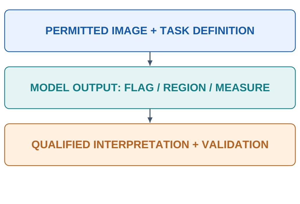
| Task | Output |
|---|---|
| Classification | Image-level category |
| Detection | Candidate location |
| Segmentation | Pixel / region boundary |
| Measurement | Numerical image-derived quantity |
4.15.1 Why a Test Can Mislead
Images from the same patient can be related.
If they appear in both development and test groups, performance may exaggerate generalization.
Different institutions or imaging protocols can change the data distribution.
A model can learn a shortcut such as an image marker or device artifact.
That pattern may correlate with labels without representing the medically relevant finding.
4.15.2 Performance and Workflow
Evaluate false positives and false negatives under the intended use.
A screening flag, triage priority and measurement tool have different practical roles.
The task must specify what the model supports.
The existence of validated devices for defined intended uses does not mean that a classroom classifier or general chatbot has equivalent validation.
| Question | Why It Matters |
|---|---|
| What is the exact intended use? | Defines the claim being assessed |
| How were labels established? | Determines reference quality |
| Which images are independent? | Reduces misleading leakage |
| Does it transfer to new conditions? | Checks distribution differences |
Describe the computing task and output, then explain the need for appropriate clinical evaluation and qualified interpretation.
4.16 Genomics
Genomics studies DNA-related information and variation.
AI can help identify patterns in sequence data, estimate effects relevant to gene regulation or prioritise research questions.
A genomic prediction is not automatically a personal-health conclusion.
Sequence data can be represented as ordered symbols and numerical features.
Models may relate those representations to measured biological outcomes.
The reference experiments, species and conditions define what an output means.

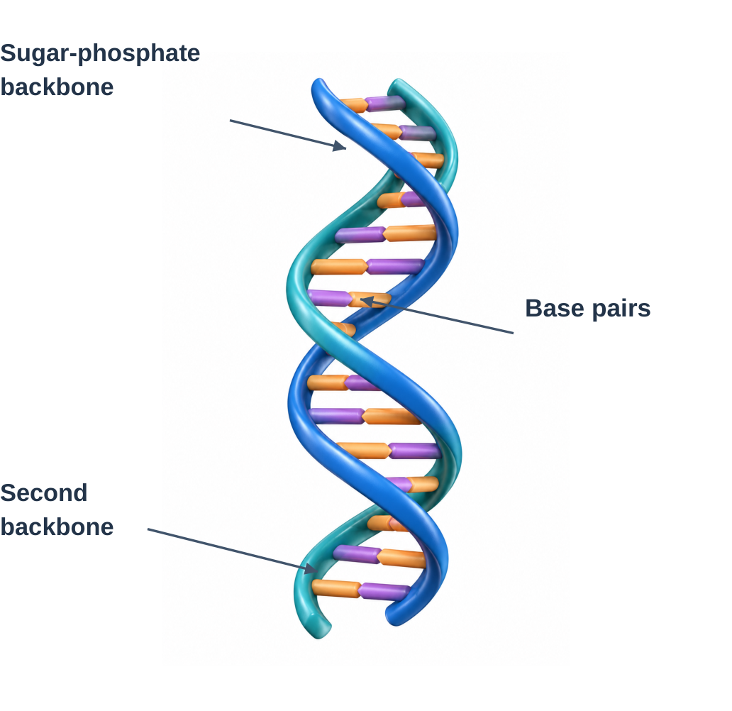
4.16.1 A Documented Research Direction
The supplied notes discuss Google DeepMind’s AlphaGenome research as an example of predicting aspects of how DNA variation relates to molecular processes such as gene regulation.
The conceptual link is sequence-to-biological-output modelling.
It is not a general guarantee of personal-genome interpretation.
Check where predictions are supported and what experimental validation remains necessary.
A computational estimate can guide a research question without settling it.
4.16.2 Wearables
Wearable devices collect repeated measurements close to the body.
AI may recognise activity, summarise patterns or flag a defined signal condition.
Inputs can include motion-related measurements or other signals supported by the device.
An activity category, wellness summary and validated medical measurement are different outputs.
Do not treat every notification as a diagnosis or every consumer device as a clinical instrument.
| Stage | Example / Consideration |
|---|---|
| Measurement | Sensor signal and collection context |
| Preparation | Handling noise and missing intervals |
| Prediction | Activity or defined pattern estimate |
| User feedback | Task-specific summary / flag |
| Check | Compare with appropriate reference observations |
Motion, device fit and wearing position can affect measurements.
Repeated samples from one person should not create an apparently independent test of generalization to new people.
Wearable histories can reveal sensitive routines.
Access, retention and sharing choices are part of system design.
4.17 AG: Precision Farming
Precision farming uses information about variation within and across fields to support targeted decisions.
AI can estimate patterns from spatial, temporal and environmental data.
It complements measurements and agronomic interpretation rather than making every field identical.
Inputs can include sensor observations, images, weather history and location-related measurements.
Outputs might be maps of variation, predicted quantities or areas requiring inspection.
An output map is not automatically an action prescription.

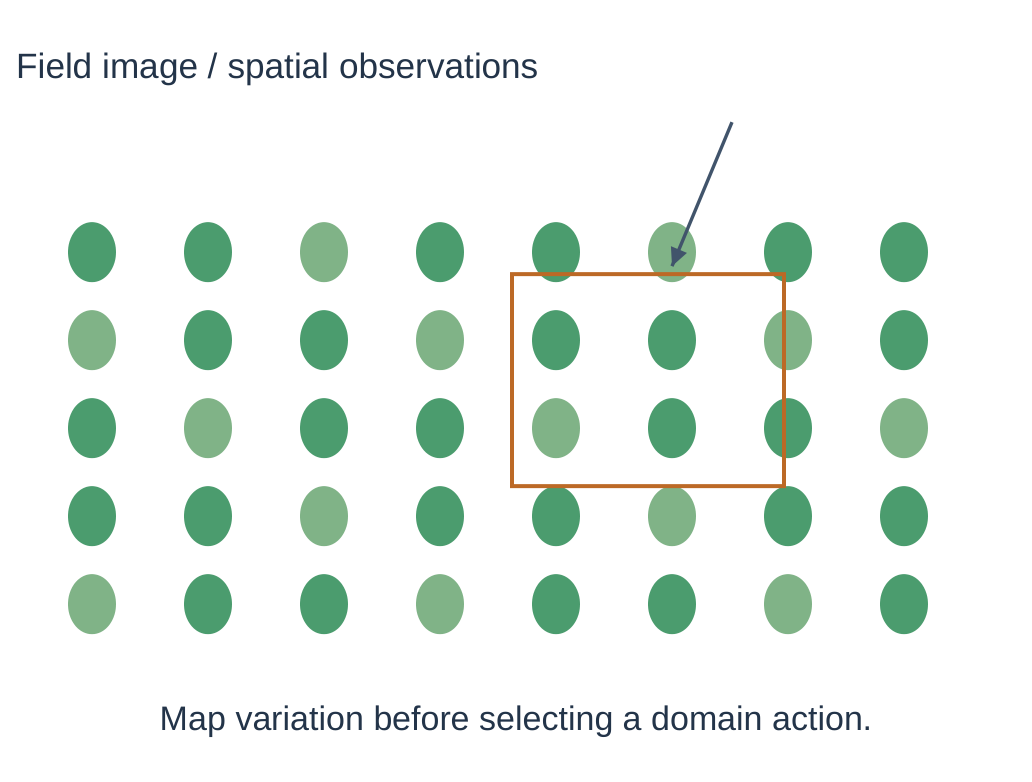
4.17.1 Why Location Matters
A field-average measurement can hide a dry region and a wet region.
Spatially resolved information supports investigation of those differences.
Measurement resolution and accuracy affect which variations can be detected.
The same region can change over time.
A map should carry collection dates and conditions so an old pattern is not treated as a current observation.
4.17.2 Decision-Support Workflow
| Step | Purpose |
|---|---|
| Measure | Observe relevant field conditions |
| Align | Match location, time and units |
| Analyse | Estimate or group patterns |
| Review | Interpret with agronomic context |
| Evaluate | Check the practical outcome |
A predicted yield is a numerical estimate.
A healthy-looking versus affected leaf decision is classification.
Clustering field measurements explores groups without preassigned target labels.
The agricultural setting does not determine the learning strategy.
Evaluate across relevant seasons, locations and crop varieties.
A model that works in one collection setting can fail when soil, weather or farming practices change.
4.17.3 A Common Data Problem
Images with different lighting may create apparent vegetation differences.
A model may map brightness rather than the condition of interest.
Use appropriate collection controls and reference measurements.
A missing observation differs from zero.
A failed sensor should not be interpreted as zero rainfall or zero moisture without a justified definition.
Nearby field samples can also be related.
If the goal is use in a new field, randomly splitting adjacent samples may exaggerate transfer performance.
4.18 Crop Monitoring and Aerial Sensing
Crop monitoring uses repeated observations to identify changes that may need investigation.
Ground images, aerial images and other measurements can support canopy mapping or visible-pattern classification.
An unusual visual pattern can have several causes.
Drones can carry sensors that gather observations from above a field.
AI helps interpret data, while location alignment and collection conditions remain essential.
The aircraft itself is not the classifier.

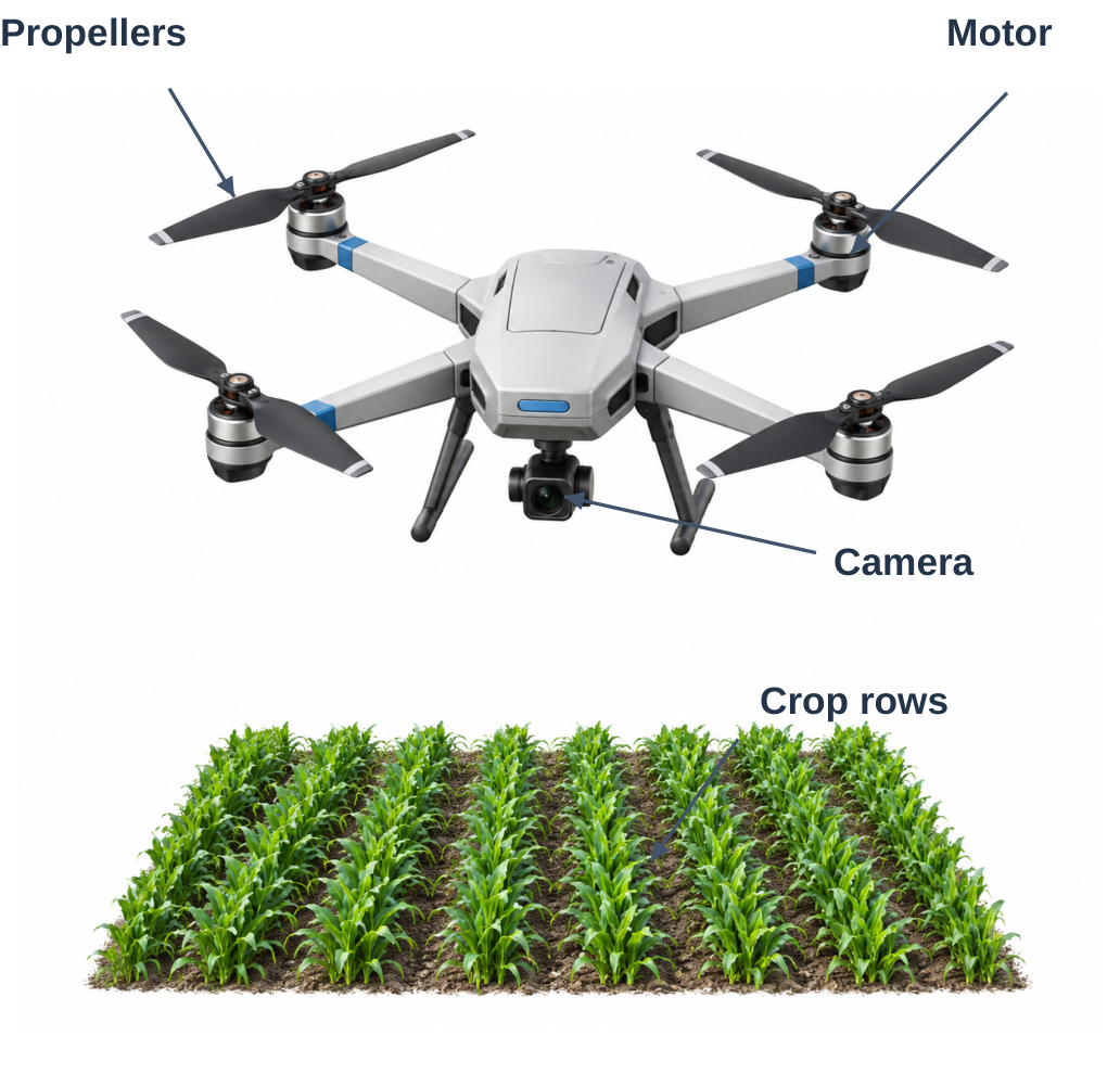
4.18.1 From Image to a Review Map
Step 1: Collect permitted observations under suitable conditions.
Step 2: Align images with location and collection time.
Step 3: Check image quality and coverage.
Step 4: Generate task-specific categories or regions.
Step 5: Confirm important findings with relevant field evidence.
4.18.2 Drone-Based Spraying: The Concept
A targeted application workflow can connect sensed variation with a defined treatment plan under applicable agronomic, environmental and operational requirements.
Detection, planning and actuation are separate stages.
A model’s visual category alone does not determine a substance, dose or permitted operation.
This example concerns information-driven targeting, not instructions for operating equipment.
4.18.3 Real Example: See & Spray
The source notes discuss John Deere’s See & Spray as a computer-vision and machine-learning example for identifying weeds and supporting targeted spraying in its intended settings.
It connects camera observations, classification and controlled actuation.
It should not be relabelled as a drone product.
The documented example is a sprayer-system application.
The shared concept is targeted use of visual information, while physical platforms and operating constraints differ.
| Component | Question |
|---|---|
| Visual model | What pattern is detected? |
| Spatial alignment | Where does the observation apply? |
| Decision rules | What actions are permitted? |
| Actuator | How is the authorised action executed? |
| Outcome check | Did the intended result occur? |
Shadows, overlap or a new crop appearance can alter the image.
An incorrect classification can propagate into later decisions unless uncertainty and outcomes are checked.
4.19 Soil Analysis and Yield Estimation
Soil-related analysis can combine measured properties, location and historical information to estimate a defined quantity or identify patterns.
Validity depends on representative sampling, measurement quality and target definition.
A visible photograph does not reveal every soil property.
If the target is laboratory-measured, suitable reference measurements are needed.
A generated description of soil colour is not a complete laboratory analysis.

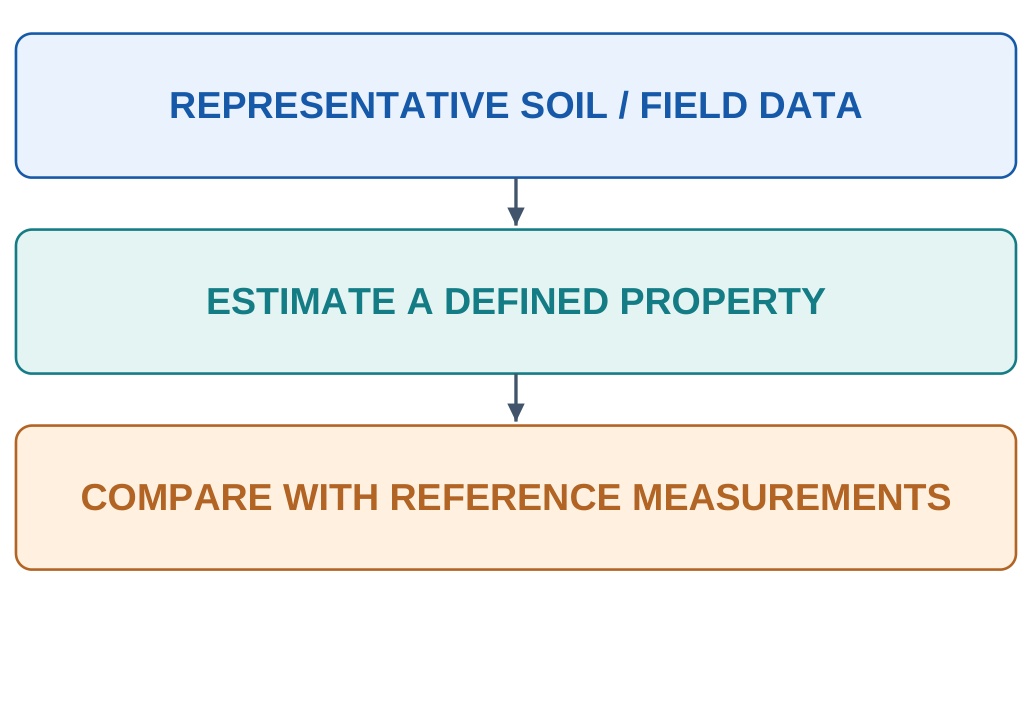
4.19.1 Sampling and Scale
Repeated readings from one small location do not automatically represent an entire field.
Sampling should reflect variation relevant to the question.
Location, depth and collection time can affect interpretation.
Use consistent units and measurement methods.
A model can learn a change in measurement practice rather than the physical relationship of interest when procedures differ systematically.
4.19.2 Yield Prediction
Yield estimation may use past field outcomes, weather-related information and management variables available before prediction.
State the prediction horizon and geographic scope.
Actual seasonal outcomes can differ because of events not represented in the input.
A prediction is an estimate, not a guaranteed harvest or a causal claim about an intervention.
| Actual | Predicted | Absolute Error |
|---|---|---|
| 4.0 | 4.4 | 0.4 |
| 5.0 | 4.8 | 0.2 |
| 6.0 | 5.7 | 0.3 |
MAE calculation
MAE = (0.4 + 0.2 + 0.3)/3
MAE = 0.3 target units
If the target is tonnes per hectare, attach that unit to actual values, predictions and MAE.
Low error on three records says little about another region or future season.
Compare a meaningful baseline and test intended deployment conditions.
Leaf-category accuracy and yield MAE measure different outputs.
Select the metric after identifying whether the target is a category, number or region.
4.20 CH: Process Optimisation
Chemical-process applications can use operating data to estimate quality, identify unusual behaviour or support optimisation.
Inputs may include temperature, pressure, flow and composition-related measurements when available.
A predictive model estimates a target quantity.
An optimiser uses objectives and constraints to compare candidates.
A control system implements permitted operating behaviour.
These components can be combined, but they perform different functions.

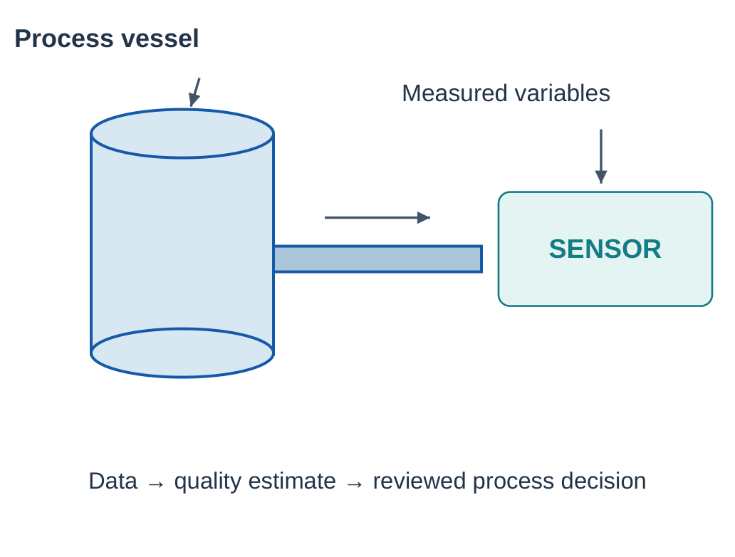
4.20.1 Soft-Sensor Idea
A soft sensor is a computational estimate of a quantity from other observations.
It can help when direct measurement is delayed or costly.
It still needs reference data and checks for changing process conditions.
A model can become inaccurate if raw-material properties or equipment condition change.
Monitoring should identify when an estimate is outside development conditions.
4.20.2 Objectives and Constraints
| Element | Illustrative Meaning |
|---|---|
| Objective | Reduce resource use while meeting quality |
| Decision variables | Permitted candidate settings |
| Constraints | Specified operating and quality limits |
| Prediction | Estimated quality / consumption |
| Verification | Independent engineering checks |
A candidate may consume less energy but fail its quality requirement.
That candidate is not a valid optimum for the constrained task.
State the feasible set before comparing a single performance number.
Historical data may cover only a narrow operating region.
Optimising a learned model beyond that region can produce attractive but unsupported predictions.
4.20.3 Quality Control
A model can screen measurements for likely off-specification output or estimate a continuous quality property.
Category decisions use classification measures.
Numerical estimates can use error measures such as MAE.
An AI-generated explanation of an anomaly remains a hypothesis unless verified.
Correlation between a variable and quality does not alone establish what would happen if that variable were changed.
4.21 TX: Textile Quality Control
Textile-inspection applications analyse surface information to identify a defined quality issue.
Camera images can support patch classification, defect detection or segmentation.
The required output depends on whether the task needs a whole-patch label, a location or a precise region.
Images should represent relevant fabric textures, colours, lighting and production conditions.
A model trained on one weave can mistake another normal texture for a defect.

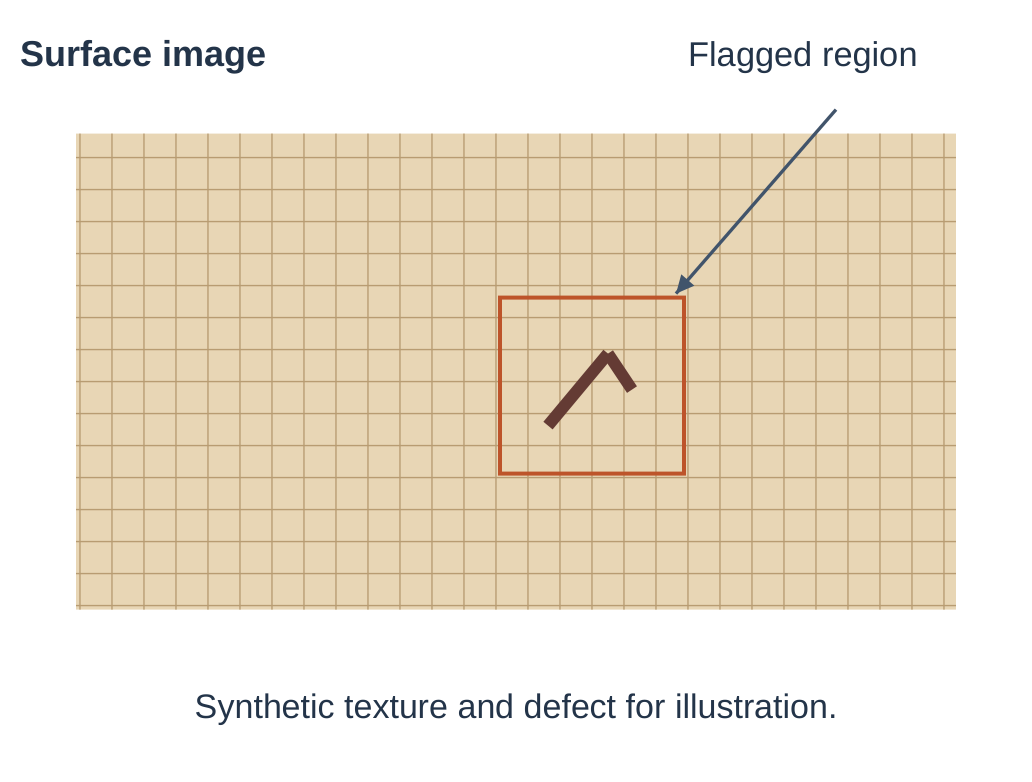
| Task | Output |
|---|---|
| Patch classification | Acceptable / defect category |
| Detection | Candidate defect location |
| Segmentation | Affected pixels / region |
| Numerical estimate | Defined size or property estimate |
4.21.1 From Images to Quality Decisions
The camera supplies measurements.
Preparation provides compatible dimensions and numerical values.
The model generates a task-specific result.
The inspection workflow decides what review is required.
For detection, a correct defect category with the wrong location can still be a failure.
For segmentation, a coarse boundary may not meet the measurement need.
Evaluate the output actually required.
4.21.2 Independent Data Groups
Patches cut from the same roll image can be closely related.
Splitting adjacent patches across training and testing can reward memorizing one texture or lighting setup.
Grouping by source roll or acquisition episode can produce a more meaningful check where appropriate.
Inspect false alarms on normal patterns and missed subtle defects.
Unequal class frequencies make overall accuracy insufficient.
| Failure Source | Possible Observation |
|---|---|
| Glare | Normal region flagged |
| New weave | Texture treated as a defect |
| Low contrast | Small defect missed |
| Repeated background | Artificially easy test split |
A visual model assesses what its sensor captures.
It does not establish every mechanical or chemical property of the textile.
Match the quality claim to available evidence.
4.22 Material Design Across CH, TX and ME
AI can help explore material candidates, estimate properties and connect composition or processing information with observed outcomes.
This supports a search process rather than replacing physical characterization.
An input representation may describe composition, process history or measured structure.
The output could be strength, thermal behaviour or another precisely defined property.
Different target properties require different reference tests and conditions.

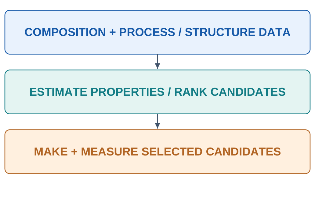
4.22.1 Multiple Objectives
A material may need to balance performance, cost, manufacturability and environmental considerations.
Improving one property can worsen another.
Explain which objective is being optimised and which requirements are constraints.
Candidate generation may suggest a composition not previously tested in the collection.
That novelty is a reason for investigation, not proof of feasibility or performance.
4.22.2 A Synthetic Selection Exercise
| Candidate | Property Criterion | Cost Criterion |
|---|---|---|
| A | Pass | Pass |
| B | Fail | Pass |
| C | Pass | Fail |
If both criteria are mandatory, only A is feasible.
B cannot win because it is cheaper if the required property fails.
C cannot win on property alone if its cost exceeds a fixed limit.
If cost is an objective rather than a hard constraint, the comparison changes.
The same numerical data can support a different decision when the problem definition changes.
4.22.3 Data Provenance and Extrapolation
Properties measured under different test conditions may not be directly comparable.
Record units, methods and relevant environmental conditions so the model does not merge unlike labels.
A prediction for a new material family may extrapolate beyond training support.
Report that uncertainty and check the candidate experimentally.
Additional decimal places in a prediction do not create new measurement precision.
Chemical, textile and mechanical examples can share property-prediction ideas.
The material system and validation change, while the input–target–check logic remains the same.
4.23 Ethical Concern: Bias
Bias can cause systematic distortions or unfair differences in performance or outcomes.
It can arise from data collection, label definitions, objectives and the way outputs are used.
Intentional prejudice is not required for a harmful difference to appear.
A city reporting app may underrepresent residents who cannot use it.
An inspection dataset may represent one material well while another is rare.
The model can appear strong overall while serving some relevant groups poorly.

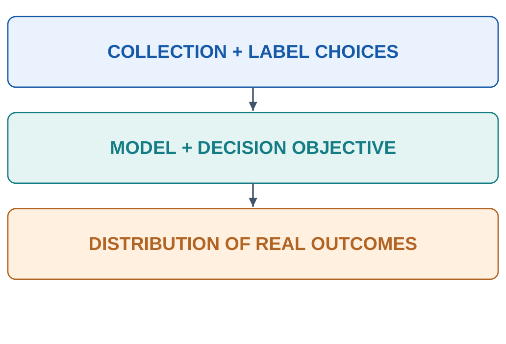
4.23.1 A Synthetic Group Comparison
| Group | Actual Cases Found | Recall |
|---|---|---|
| A | 90 of 100 | 90% |
| B | 50 of 100 | 50% |
| Combined | 140 of 200 | 70% |
The combined recall hides a large difference.
This invented table shows why one overall measure can be insufficient.
It does not establish the cause of the gap or describe a real population.
4.23.2 How to Investigate
- Identify relevant populations or operating groups.
- Check representation and reference-label quality.
- Compare suitable error measures and sample sizes.
- Investigate collection and operating differences.
- Provide a correction route for affected users.
- Reassess after changes in data or deployment.
Removing a group label does not guarantee fairness.
Other variables can act as proxies, and unequal collection patterns can remain.
A mitigation should be tested rather than assumed to work because it sounds neutral.
Fairness also depends on the decision context.
Equal average errors may not address unequal service access or an inappropriate objective.
4.23.3 Explainability and Accountability
An explanation helps a reviewer understand a prediction’s basis or workflow assumptions.
It does not prove correctness.
A simple but inaccurate explanation can mislead.
Accountability identifies who owns decisions, monitors performance and responds to errors.
“The AI decided” is not a complete explanation of responsibility for a deployed engineering system.
4.24 Ethical Concern: Data Privacy
Engineering data can contain personal or confidential information even when it looks technical.
Location traces, wearable signals, images and service histories can reveal identities, routines or sensitive circumstances.
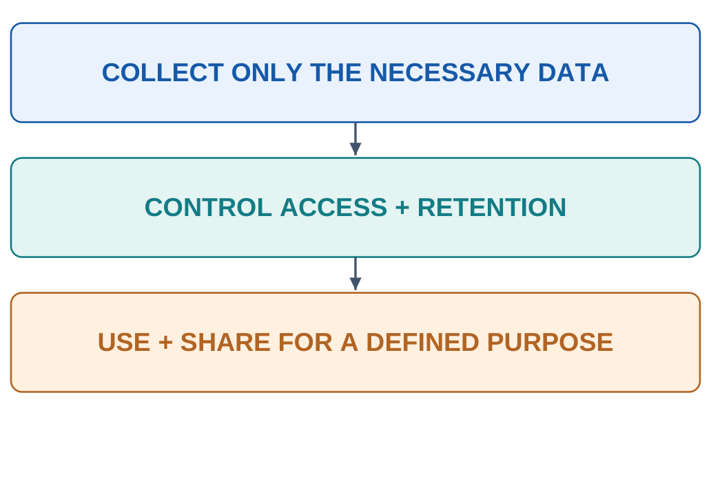
Privacy requires considering:
- What data is necessary.
- Who can access it.
- How long it is retained.
- What is shared.
- Which purpose justifies its use.
Collecting every available field is not automatically justified by the possibility of training a model.

| Data | Possible Sensitivity |
|---|---|
| Travel history | Locations and routines |
| Wearable history | Activity and health-related patterns |
| Camera images | Identifiable people / surroundings |
| Factory records | Confidential process information |
4.24.1 Anonymisation and Access
Removing names can reduce direct identification but may not remove all identifying information.
A combination of locations or rare attributes can still be revealing.
Treat anonymisation as a process to assess rather than a universal guarantee.
Access should match roles and purpose.
A person allowed to read a maintenance summary may not need the entire raw dataset.
A classroom demonstration can use synthetic examples instead of private operational records.
4.24.2 Security and Privacy Differ
Security protects systems and data against unauthorised access or alteration.
Privacy concerns whether and how information about people is collected and used.
A securely stored dataset can still be used for an inappropriate purpose.
A locally run model does not automatically make the whole workflow private.
Logs, backups or shared outputs can still expose information.
Hosted-service behaviour depends on actual terms and configuration.
| Question | Design Implication |
|---|---|
| Do we need this field? | Minimise unnecessary collection |
| Who needs the raw record? | Limit access |
| When should it be removed? | Define retention |
| Can a synthetic example work? | Avoid needless exposure |
| What is sent to another service? | Inspect the actual workflow |
4.25 Job Displacement and Changing Skills
AI can automate some tasks, change how work is divided and create demand for different skills.
Task automation and elimination of an entire occupation are different claims.
Outcomes depend on adoption, institutions, costs and work reorganisation.
In inspection, a model may screen images while staff investigate difficult cases.
In software development, drafting can be accelerated while requirements and review remain.
Neither example proves that every job disappears or remains unchanged.
| Change | Possible Effect |
|---|---|
| Routine drafting assistance | More time for review / problem definition |
| Automated screening | New need to inspect difficult cases |
| New data workflow | Demand for measurement and evaluation skills |
| Poorly managed transition | Unequal access to reskilling and opportunities |
4.25.1 Skills That Support Responsible Use
- Define an engineering problem precisely.
- Understand measurements and units.
- Evaluate outputs using appropriate evidence.
- Recognise uncertainty and data limitations.
- Communicate findings and retain accountability.
- Keep learning tools and domain fundamentals.
4.25.2 Responsible AI Through the Lifecycle

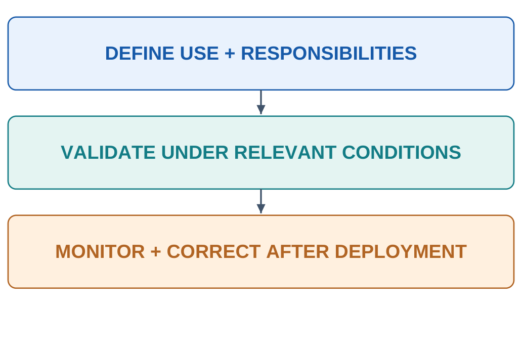
A responsible system has a clear intended use, appropriate data, meaningful evaluation and a failure-handling process.
Domain experts and affected users can reveal issues a headline metric misses.
Human oversight requires more than putting a person’s name on a flowchart.
The reviewer needs relevant information and a realistic ability to question or override unsupported recommendations.
4.25.3 A Practical Review
- What is the intended benefit and who receives it?
- Which errors or exclusions matter?
- Who monitors performance and investigates complaints?
- What happens when the model is uncertain or unavailable?
- How are changes documented and checked?
Discuss benefits and limitations together.
Avoid unsupported forecasts about salaries, total job loss or guaranteed career outcomes.
Explain the skills and design decisions a student can develop.
4.26 Real Case and Group Activity
The syllabus asks each group to present a real AI application from its engineering domain in two minutes.
Groups of three or four can divide work into evidence collection, technical explanation, impact assessment and presentation.
Submit notes or slides plus a one-page handout as required.
A real case needs an identifiable system and public evidence.
Distinguish the provider’s reported result from a result independently measured by the group.
Use a conceptual schematic if internal details are not public.
4.26.1 Historical Case: Data-Centre Cooling
The supplied notes discuss Google and DeepMind’s historical use of machine learning to support data-centre cooling optimisation.
Their 2016 account reported a reduction of up to 40% in energy used for cooling in the described work.
This is a reported case result, not a guarantee for another facility or a claim about total electricity use.
The engineering connection is measurements, learned estimates and constrained operational decisions.
The example connects ME, EE and CH interests in thermal systems, energy and process operation.
| Element | Case-Study Focus |
|---|---|
| Problem | Energy used for cooling |
| Data | Relevant operating and environmental measurements |
| AI role | Predictive / optimisation support |
| Impact | Reported cooling-energy reduction |
| Limit | Scope and operating conditions matter |
The percentage concerns cooling energy in the reported setting.
It must not be rewritten as a 40% reduction in every data centre’s total electricity use.
4.26.2 Two-Minute Presentation Plan
| Time | Content |
|---|---|
| 0–20 s | Name the problem and real system |
| 20–50 s | Describe input data and collection |
| 50–85 s | Explain model output and workflow |
| 85–110 s | Discuss reported impact and evidence |
| 110–120 s | State one limitation / open question |
The intervals total 120 seconds.
Practise the talk rather than filling it with product names.
A labelled input–model–output diagram communicates the technical idea quickly.
Other case choices discussed in the supplied notes include Project Green Light, maintenance systems, the Airbus–Autodesk design project, AlphaFold and See & Spray.
Check the selected case’s actual scope before presenting it.
4.26.3 One-Page Handout
Include:
- Application name and branch connection.
- Problem, data, AI output and decision.
- One clear labelled schematic.
- Reported impact with its scope explained.
- One limitation and a discussion question.
If exact architecture or training data is not public, say so.
Do not invent a network size, customer result or private dataset to complete a template.
4.27 Quick Revision and Exam Practice
| Domain | Main Tasks to Recall |
|---|---|
| CE | Structural monitoring, city services, traffic |
| ME | Maintenance, constrained design, robotics |
| EE | Demand / generation forecasting, faults |
| ECE | Sensing, fault analysis, VLSI assistance |
| CSE | Code assistance, cybersecurity, interfaces |
| BT / healthcare | Discovery research, imaging, genomics, wearables |
| AG | Precision farming, crops, aerial sensing, soil |
| CH | Process prediction and optimisation |
| TX | Visual inspection and material quality |
4.27.1 Short-Answer Questions
- Distinguish detection, classification and localisation.
- Why is an anomaly not a complete diagnosis?
- Contrast reactive, preventive and predictive maintenance.
- Name two objectives or constraints in design optimisation.
- Why is a smart-grid forecast not a control rule?
- Differentiate image classification and segmentation.
- Why does spatial variation matter in farming?
- How can an overall average hide unequal performance?
- Distinguish data security and privacy.
- Why is task automation different from job elimination?
- What is a soft sensor?
- Why must a predicted material property be independently checked?
4.27.2 Longer-Answer Questions
- Explain structural health monitoring using inputs, model output, inspection workflow and limitations.
- Discuss predictive maintenance and design optimisation with one worked example each.
- Describe smart-grid and VLSI applications, distinguishing prediction from verification.
- Explain code generation, defensive cybersecurity and natural-language interfaces.
- Compare drug-discovery research, medical imaging, genomics and wearables.
- Describe precision farming, crop monitoring, aerial sensing and soil analysis.
- Explain process optimisation, textile inspection and material design.
- Discuss bias, privacy, job displacement and responsible oversight using branch examples.
4.27.3 Numerical and Reasoning Checks
Traffic
50 s to 40 s is 10 s lower.
Relative reduction = 10/50 × 100 = 20%.
The change alone does not prove a causal AI benefit.
Fault screening
16 true positive flags, 4 misses and 8 false flags give:
Recall = 16/20 = 80%
Precision = 16/24 ≈ 66.7%
Yield example
Errors 0.4, 0.2 and 0.3 give:
MAE = 0.3 target units
Design
A lighter candidate failing a mandatory constraint is not feasible.
Case study
Identify problem, data, AI output, decision and evidence before describing impact.
Start an answer with task and data, explain the model’s role, draw a labelled flow, discuss validation and give one concrete limitation.
COMPLETE EXPLANATIONS FOR EXAM ANSWERS
The following answers connect the applications in these AI and Prompt Engineering Unit 4 Notes.
Explain Structural Health Monitoring with an AI Workflow
Structural Health Monitoring collects information about a structure’s condition over time.
Inputs can include vibration, strain, displacement, temperature and images.
A model may estimate expected response, flag unusual behaviour or locate a visible crack.
Establish a relevant baseline, collect consistent time-stamped measurements, check sensor quality, prepare representations and compare current observations with expected patterns.
Flagged cases support inspection. They do not automatically establish structural safety or a physical cause.
A model trained only on cool-morning observations may treat normal hot-afternoon behaviour as anomalous.
Evaluate environmental and loading conditions, separate relevant time periods and avoid near-duplicate-image leakage.
Qualified engineering assessment remains distinct from screening output.
Compare Predictive Maintenance and Design Optimisation
Predictive maintenance uses condition and historical records to estimate maintenance needs before a defined future event.
It differs from reactive repair after failure and preventive servicing at fixed intervals.
Vibration, load and temperature can support anomaly flags, fault categories or remaining-life estimates.
Define the warning horizon and evaluate missed events, false alarms and useful lead time.
An alarm arriving after the event does not demonstrate advance prediction.
Changed equipment or conditions can invalidate previously useful patterns.
Design optimisation compares candidates under objectives and constraints.
In the synthetic bracket table:
A weighs 1.0 kg and passes.
B weighs 0.8 kg and fails.
C weighs 0.9 kg and passes.
C is the lowest-mass feasible option among these three.
B cannot win solely because it is lighter.
Learned surrogate predictions can help search, but selected designs still require independent verification.
Explain Smart-Grid Forecasting, Fault Detection and VLSI Assistance
A smart-grid forecast estimates future demand or generation from available history and context.
It supports scheduling, but physical constraints, reserves and operational responsibility determine permitted actions.
Compare the same horizon and held-out periods against a meaningful baseline.
Fault detection flags evidence of an abnormal condition.
Classification assigns a known category.
Localisation estimates where it occurs.
Diagnosis investigates cause.
For 16 correctly flagged faults, 4 missed faults and 8 false flags:
Recall = 16/20 = 80%
Precision = 16/24 ≈ 66.7%
Finding faults and limiting false flags are different concerns.
VLSI assistance can score or search candidate layouts under area, timing, power, routing and design-rule constraints.
A predicted good score does not establish logical correctness or physical feasibility.
Explain the specific design stage and separate verification.
Explain CSE Applications Without Confusing Prediction with Execution
Code generation produces a candidate implementation from a specification and allowed context.
Review syntax, functional behaviour, input handling and security.
For a mean-calculation program, test a normal list, one value, an empty list and malformed input according to the contract.
Generated tests can share the implementation’s mistake.
Important expected results should be independently justified.
Defensive cybersecurity models can classify messages, flag unusual events or prioritise alerts.
A suspicious event is not proof of an attack or a person’s identity.
Evaluate relevant threats, false alarms, changing patterns and permitted data use.
A natural-language interface connects interpretation to retrieval or authorised actions.
Correct wording does not compensate for retrieving the wrong course notes or bypassing access rules.
Check interpretation, source selection, permission and execution separately.
Compare Biotechnology, Healthcare and Agricultural Applications
Drug-discovery models estimate molecular properties and prioritise candidates for experiments.
Protein-structure prediction and genomic models provide research estimates under defined conditions.
These outputs alone do not establish an approved medicine, full biological mechanism or personal diagnosis.
Medical-image applications may classify an image, detect a region, segment a boundary or estimate a measurement.
Patient-level independence, reference quality, device differences and intended-use validation matter.
Wearable activity categories, wellness summaries and validated medical measurements are different outputs.
Agricultural models can map spatial variation, classify visible patterns or predict yield.
Align location, time and units.
Evaluate relevant seasons, fields and crop conditions.
An aerial platform gathers measurements, a model interprets them and a decision workflow determines permitted action.
A map or high score is not automatically an agronomic prescription.
Explain Process Optimisation, Textile Inspection and Material Design
Process models estimate quality or consumption from measured variables.
A soft sensor estimates a quantity from other observations when direct measurement is delayed or costly.
Optimisation compares permitted settings under quality and operating constraints.
Correlation alone does not establish what an intervention would cause.
Textile inspection can classify a patch, detect a defect or segment affected pixels.
The output and reference labels must match the claim.
Split related roll images appropriately.
Inspect false alarms on normal texture and missed subtle defects.
Material models connect composition, processing or structure to defined properties.
Use comparable measurement methods and report extrapolation beyond training support.
Candidate generation guides physical investigation.
Experimental characterization determines whether requirements are met.
Discuss Bias, Privacy and Workforce Effects
Bias can arise through collection, labels, objectives and use.
An overall score can conceal differences across relevant groups.
Investigate representation, reference quality, sample size and deployment conditions.
Removing a group label does not guarantee fairness.
Privacy concerns what information is collected, accessed, retained and used.
Security protects against unauthorised access or alteration.
A securely stored dataset can still serve an inappropriate purpose.
Removing names alone may not remove identifying patterns.
AI can automate tasks, change work allocation and create different skill needs.
This does not establish that every occupation disappears or remains unchanged.
Students should develop problem definition, measurement knowledge, evaluation, uncertainty awareness and accountable communication.
Meaningful oversight requires information and authority to question an output.
NUMERICAL AND DECISION SHEET WITH CONDITIONS
| Check | Calculation / Interpretation |
|---|---|
| Traffic-delay difference | 50 s − 40 s = 10 s lower |
| Relative delay reduction | (10/50) × 100 = 20% in the synthetic comparison |
| Causal limitation | A before–after difference alone does not establish an AI-caused improvement |
| Fault recall | 16/(16 + 4) = 80% |
| Fault precision | 16/(16 + 8) ≈ 66.7% |
| Forecast absolute error | Actual 125 versus predicted 120 gives 5 target units |
| Yield MAE | (0.4 + 0.2 + 0.3)/3 = 0.3 target units |
| Group A recall | 90/100 = 90% |
| Group B recall | 50/100 = 50% |
| Combined recall | 140/200 = 70%; hides the group difference |
| Bracket selection | Choose C among the stated candidates when lower mass is the objective and the constraint is mandatory |
| Material feasibility | If property and cost criteria are mandatory, only candidate A passes both in the stated exercise |
| Presentation timing | 20 + 30 + 35 + 25 + 10 = 120 seconds |
Memory check: Define the task, identify available data, state the output, name the decision, choose a relevant check and explain one limitation.
QUICK REVISION: EXPLAIN AND CONNECT
Is an Anomaly a Complete Diagnosis?
No. It is a deviation under a chosen model.
Sensor faults, environmental changes and physical problems may need different investigations.
Does a Good Forecast Authorise a Control Action?
No. A forecast supplies an estimate.
Operational decisions still need constraints, responsibility and suitable checks.
Can the Lightest Design Always Win?
No. A candidate failing a mandatory constraint is infeasible, even when it has the best value on one objective.
Does Correctly Naming a Defect Locate It?
No. Classification, detection and segmentation have different outputs.
They need matching references and evaluation.
Why Are Near-Duplicate Test Examples a Problem?
They can reward recognition of development examples instead of demonstrating transfer to new assets, patients, rolls or fields.
Is a Research Prediction an Experimentally Established Result?
No. Molecular, genomic and material predictions guide investigation and need appropriate independent evidence.
Does Removing Names Guarantee Privacy?
No. Locations, routines and rare attributes can still reveal information.
Assess the complete record, access and purpose.
Does Task Automation Prove Job Elimination?
No. A job combines several tasks and responsibilities.
Adoption, workflow changes and institutions affect outcomes.
What Makes Human Oversight Meaningful?
A reviewer needs relevant information, time, competence and authority to question or correct the recommendation.
How Should a Real Case Be Presented?
Identify the actual system, problem, data, AI role, decision, reported impact and limitation.
Preserve the scope of reported numbers and distinguish them from your own measurements.
Use these AI and Prompt Engineering Unit 4 Notes to revise each branch through the same problem–data–output–decision–validation pattern. Additional unit-wise resources are available at www.notesgallery.com. The university website is https://aktu.ac.in.