
Course: AKTU B.Tech First Year | Semester I & II
Course Codes: AAS101A–AAS101I | AAS201A–AAS201I
Streams: CSE, EE, ECE, CE, ME, BT, CH, TX & AG
Unit IV Overview
Study guided light and lasers, ultrasonic generation and detection, dielectric and magnetic response, Hall measurements, thermal processes and agricultural environmental physics. Unit IV differs across streams: the branch guide identifies the topics and section numbers prescribed for your branch.
Topics Covered
| Topic | Pages |
|---|---|
| Optical fibres and laser systems | 3–10 |
| Ultrasonics and textile applications | 10–13 |
| Dielectric and magnetic materials | 13–17 |
| ME electrical properties and Hall effect | 17–20 |
| Thermal physics and heat transfer | 20–25 |
| Agricultural environmental physics | 25–29 |
| Derivations, formulas and revision | 29–34 |
Learning Outcomes
- Explain fibre guidance, optical loss and laser operation with labelled diagrams.
- Connect ultrasonic transducers with resonance, coupling and echo detection.
- Distinguish material storage, loss, switching and carrier measurements.
- Apply heat-transfer and thermodynamic relations with consistent models.
- Interpret radiation, crop microclimate, weather and pollutant balances.
Included in These Notes
50 solved problems with methods and physical checks; 38 labelled diagrams; complete derivations; a formula sheet and answered revision checks.
Study Approach
Choose your route. Read the branch guide to match your branch, course codes and official Unit IV topics.
Trace the process. Follow rays, excitation paths, acoustic signals, fields and thermal boundaries.
Check the model. State angle references, polarity, loss conventions, units and boundary conditions.
Practise and revise. Solve your route’s cases, then reproduce key derivations and physical checks.
Coverage note: The combined volume supports all nine streams with different Unit IV routes. The branch guide separates prescribed topics from supporting detail.
Unit IV: Branch and Topic Guide
Each row pairs the same within-stream syllabus in semesters I and II. The official Unit IV title and assigned sections identify your prescribed reading; supporting details are distinguished below.
| Stream / Codes | Official Subject Title | Official Unit IV / Sections |
|---|---|---|
| CE — AAS101A / AAS201A | Physics for Sustainable Structural Systems | Thermal Physics — 26–33 |
| ME — AAS101B / AAS201B | Physics of Materials | Electrical and Magnetic Properties — 19–25; dielectric support in 16–18 |
| ECE — AAS101C / AAS201C | Quantum Physics and Electronic Sensors | Dielectric and Magnetic Materials — 16–21 |
| EE — AAS101D / AAS201D | Physics of Electrical Engineering Materials | Dielectric and Magnetic Materials — 16–21 |
| CSE — AAS101E / AAS201E | Quantum Physics and Applications | Photonics — 1–11 |
| BT — AAS101F / AAS201F | Physics of Materials and Biomaterials | Photonics — 1–11 |
| CH — AAS101G / AAS201G | Physics of Process Engineering Materials | Thermal Physics — 26–33 |
| AG — AAS101H / AAS201H | Physics of Agricultural Systems and Environment | Environmental Physics — 34–40 |
| TX — AAS101I / AAS201I | Physics of Fibres and Textile Materials | Ultrasonics and Photonics — 1–4, 6, 8–15; see guidance below |
CSE and BT: Fibre structure/propagation, acceptance angle/cone/NA, attenuation and coefficient; radiation interactions, Einstein coefficients, laser principle, ruby, He-Ne and applications (1–11). Mode/dispersion and threshold calculations are supporting depth within that route.
TX: Fibre foundation and acceptance (1–3), radiation interactions (6), laser components and ruby/He-Ne/textile uses (8–11), and all ultrasound generation/detection/textile applications (12–15). Section 4 is mode/dispersion enrichment; attenuation coefficients (5) and explicit Einstein-coefficient analysis (7) are not separately listed in TX Unit IV. The threshold in 8 is supporting depth.
EE and ECE: Dielectric vectors, susceptibility, polarisation mechanisms and applications (16–18); magnetic susceptibility and classes, hysteresis/loss, coercivity, remanence and applications (19–21).
ME: Magnetic classes/applications (19–21), bands, electrical classes, dielectrics, piezoelectricity, ferroelectricity, Hall effect and carrier concentration (22–25); 16–18 provide dielectric background.
CE and CH: Laws, all heat-transfer modes, heat capacity, expansion/conductivity, melting/solidification, resistance, enthalpy/entropy, state equations and Newton cooling (26–33).
AG: Solar and crop interaction, microclimate, weather, greenhouse effect/climate change, air and water pollution (34–40). CH uses suffix G from the supplied course scheme.
1. A. Optical Fibres: Structure and Guidance
CSE and BT photonics; TX fibre foundation. An optical fibre guides light along a transparent core surrounded by optical cladding. In a conventional step-index fibre, core refractive index n1 exceeds cladding index n2. An outer polymer coating supplies protection but is not the same layer as the optical cladding.
The ray model describes meridional rays repeatedly reflecting at the core-cladding boundary. The full physical explanation is a guided electromagnetic mode satisfying boundary conditions. The ray model is especially useful for introductory acceptance-angle calculations but is not an exact description of every small-core fibre.
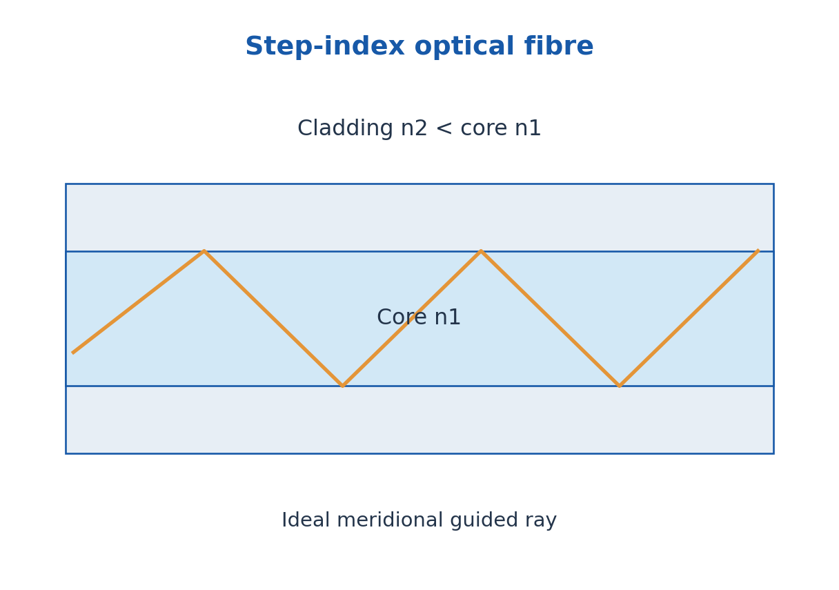
Light entering a fibre must be coupled into its guided paths or modes. A high-quality fibre does not recover light that was never coupled into it. Source alignment, connector condition, end-face preparation and bend radius can therefore influence a practical link as much as the ideal material indices.
Fibres offer compact flexible transmission and are used in communication, illumination and sensing. They carry optical energy rather than electric current along the glass core. A fibre sensing arrangement needs a specific transduction and readout mechanism; a generic cable is not automatically a calibrated temperature or strain instrument.
2. Refraction, Critical Angle and Propagation Conditions
Snell’s law is nA sin i = nB sin r, with angles measured from the interface normal. Total internal reflection requires incidence from the higher-index material toward the lower-index material and incidence angle greater than the critical value ic = sin^-1(n2/n1). The critical angle exists only when n1 > n2.
At the limiting angle, the refracted ray is tangent to the boundary. Beyond it, there is no propagating refracted ray in the elementary model, although an evanescent field extends into the cladding. Total internal reflection therefore does not mean the electromagnetic field is mathematically zero immediately beyond the interface.
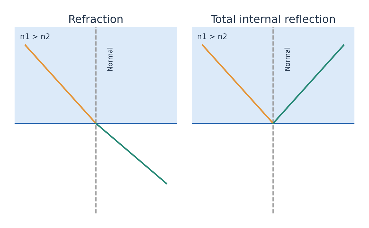
For a straight fibre meridional ray, the internal incidence angle to the cylindrical boundary normal is complementary to its angle to the fibre axis. A ray too steeply inclined to the axis may fail the guidance condition. Entrance angle to the axis and internal angle to the normal are different quantities.
Draw the normal at the actual interface before inserting a trigonometric function. A bend can change local incidence and increase radiation loss. The ideal guidance derivation assumes a straight uniform fibre, an appropriate entrance face and negligible imperfections.
Worked Problem 4.1: Internal Critical Angle
Problem: A fibre has n1 = 1.50 and n2 = 1.47. Find the internal critical angle at the core-cladding interface.
Method: ic = sin^-1(n2/n1), measured from the normal.
Calculation: Evaluate sin^-1(1.47/1.50).
Answer: ic = 78.5217 degrees.
Check: This is not the entrance angle relative to the fibre axis.
3. Acceptance Angle, Cone and Numerical Aperture
The acceptance half-angle θa is the largest ideal external meridional entrance angle measured to the fibre axis. Let the surrounding entrance medium have refractive index n0. At the limiting guided ray, combining entrance Snell refraction and the internal critical-angle geometry gives n0 sinθa = √(n1² – n2²).
The numerical aperture is NA = n0 sinθa. It is dimensionless and describes the ideal acceptance relation under the step-index assumptions. In air, n0 is approximately one; in water or another coupling medium, divide NA by n0 before taking the inverse sine.
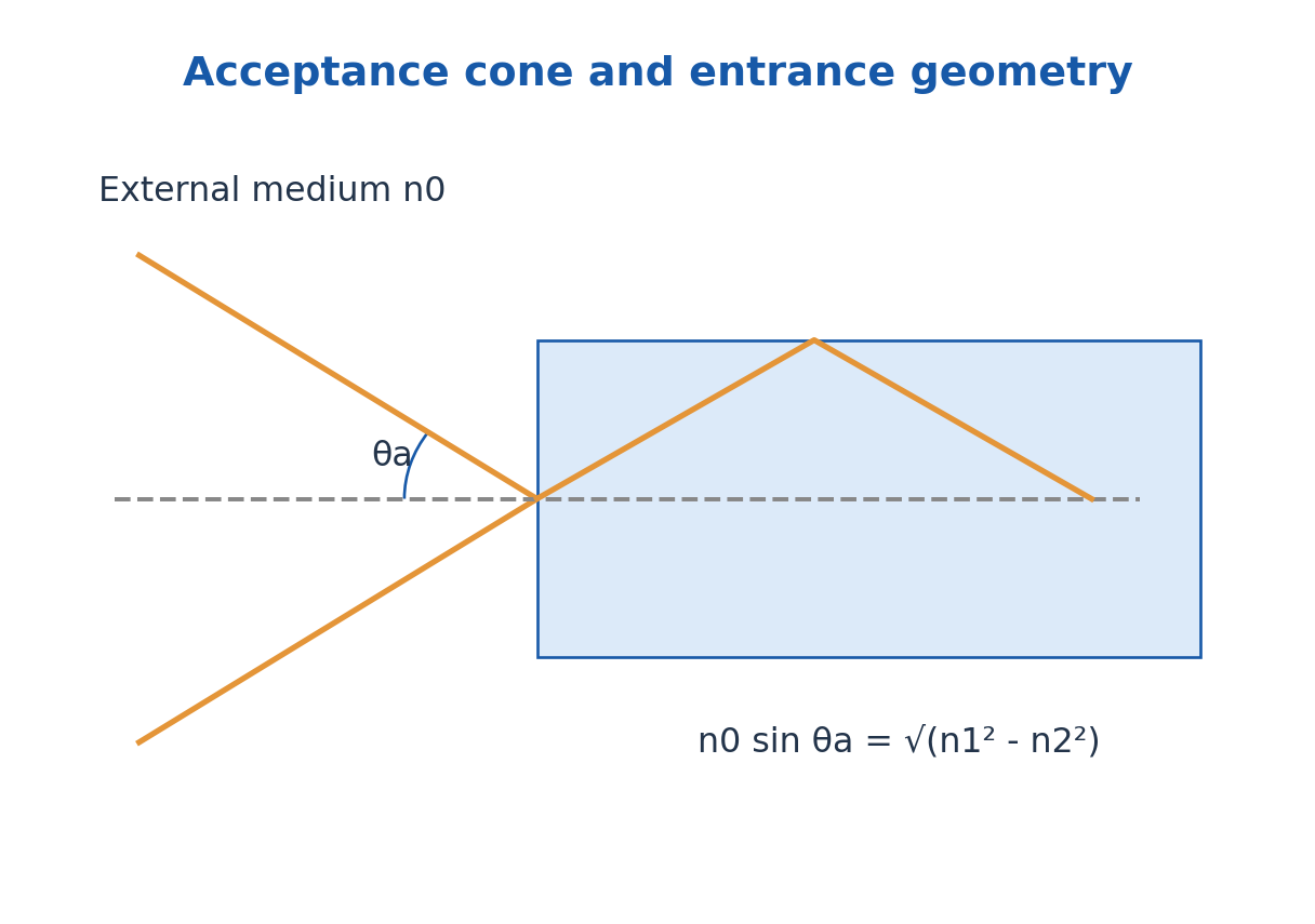
The acceptance cone has full apex angle 2θa. If the relative core-cladding index difference is Δ = (n1 – n2)/n1 and is small, NA ≈ n1√(2Δ). The exact square-root difference should be used when the small-Δ approximation is not justified.
Numerical aperture and collected power are related but not interchangeable. Power also depends on the source angular distribution, area, alignment and mode coupling. An acceptance angle alone does not specify a complete link budget.
Worked Problem 4.2: NA and the Full Acceptance Cone
Problem: For the same fibre in air, find NA, entrance half-angle and full cone angle.
Method: NA = √(n1² – n2²); θa = sin^-1(NA) in air.
Calculation: Use squared indices before taking the square root.
Answer: NA = 0.29850; θa = 17.3673 degrees; full cone = 34.7346 degrees.
Check: The cone angle is twice the half-angle; it is not twice the critical angle.
Worked Problem 4.3: Immersed Fibre Entrance
Problem: The preceding fibre end is immersed in a medium of index 1.33. Find entrance half-angle using the unchanged ideal NA.
Method: sinθa = NA/n0.
Calculation: Divide the previous NA by 1.33 before taking the inverse sine.
Answer: θa = 12.9696 degrees.
Check: The higher external index reduces the entrance half-angle under the ideal model.
Worked Problem 4.4: Small Index-Difference Estimate
Problem: For n1 = 1.50 and n2 = 1.47, compare n1√(2Δ) with the exact NA.
Method: Δ = (n1 – n2)/n1; NAapprox = n1√(2Δ).
Calculation: Δ = 0.0200; evaluate both formulas.
Answer: Approximate NA = 0.30000; exact NA = 0.29850; approximation is 0.5038% higher.
Check: The approximation is justified by small Δ, not by the numerical size of the entrance angle alone.
4. Fibre Profiles, Modes and Dispersion
A step-index profile changes abruptly at the core boundary. A graded-index profile decreases through the core, giving curved ray paths in the geometric model. In a suitable multimode design the changing speed along different paths reduces intermodal delay compared with a comparable step-index multimode fibre.
A single-mode fibre supports one spatial mode over the stated operating range, with polarisation structure treated separately. A multimode fibre supports several spatial modes. The approximate step-index normalised frequency is V = (2πa/λ)NA; the familiar V < 2.405 single-mode condition refers to the ideal weakly guiding circular fibre.
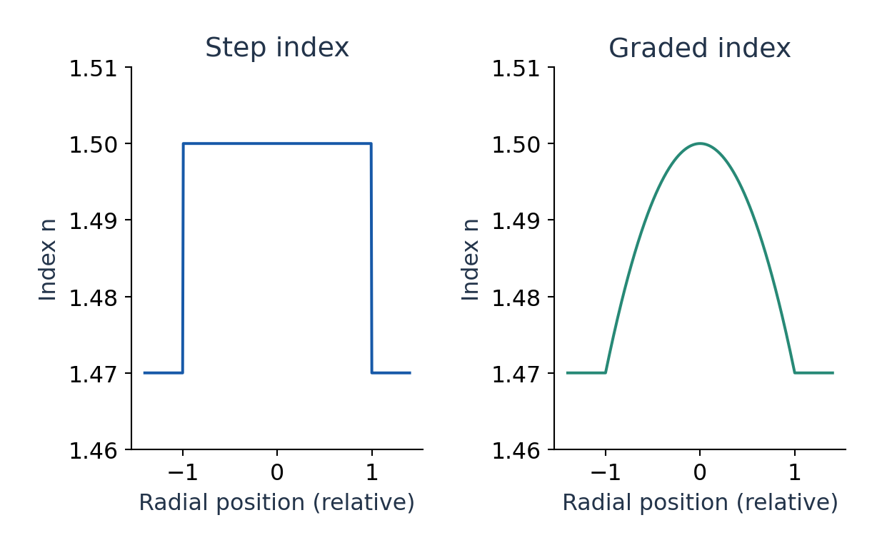
Intermodal dispersion comes from different modal delays. Material dispersion comes from refractive-index dependence on wavelength; waveguide dispersion comes from the guided structure. A finite source spectrum can therefore broaden a pulse even in a single-mode link.
Pulse broadening and attenuation are distinct limitations. A strong but badly broadened pulse can overlap neighbours; a narrow pulse can still be too weak to detect. These mode and dispersion details support the common fibre syllabus rather than replacing its prescribed acceptance and propagation derivations.
Worked Problem 4.5: Ideal Single-Mode Check
Problem: A weakly guiding circular step-index fibre has core radius 4.0 micrometres, NA = 0.10 and wavelength 1550 nm. Evaluate V and compare with 2.405.
Method: V = (2πa/λ)NA.
Calculation: Use a = 4 × 10^-6 m and λ = 1.55 × 10^-6 m.
Answer: V = 1.62147, below 2.405; the ideal single-spatial-mode condition is met.
Check: This is supporting mode theory; the cutoff assumes the specified ideal circular weak-guidance model.
Worked Problem 4.6: Pulse Broadening Estimate
Problem: A link model gives chromatic dispersion D = 17 ps/(nm km), length 8.0 km and source width 0.20 nm. Estimate broadening magnitude.
Method: Δt ≈ |D|LΔλ.
Calculation: 17 × 8.0 × 0.20 = 27.2 ps.
Answer: Estimated broadening = 27.2 ps.
Check: This linearised spectral estimate is distinct from power loss and excludes other broadening mechanisms.
5. CSE and BT: Attenuation and Optical Link Budgets
Attenuation describes loss of guided optical power with distance through absorption, scattering and radiation or bending effects. In the exponential power model P(L) = P0 exp(-αp L), αp is a power attenuation coefficient in inverse length. A field-amplitude coefficient would use a different factor in its exponent.
Decibel loss is A = 10 log10(Pin/Pout), and distributed loss is αdB = A/L. Thus αdB = 4.343αp when the same length unit is used. Conversely, Pout = Pin × 10^(-A/10). A positive passive loss decreases power; a gain factor is a different sign convention.
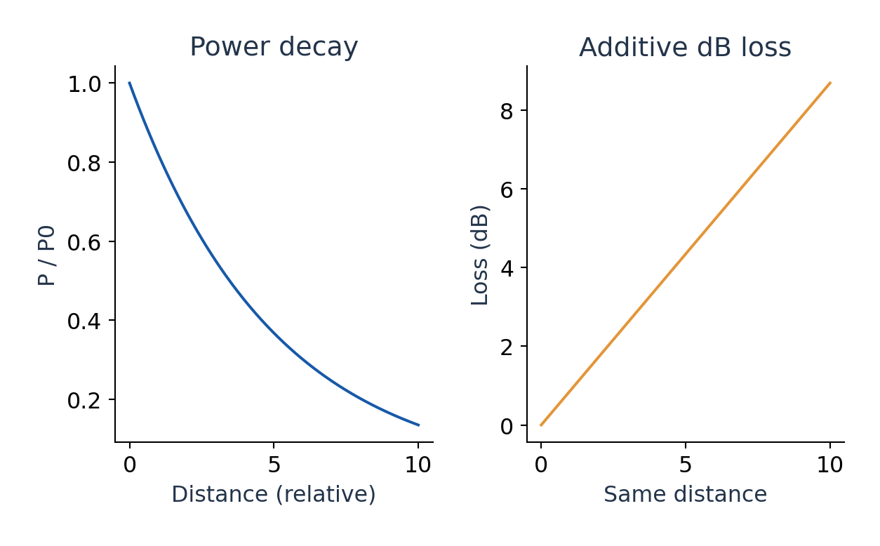
Fibre, splice and connector losses add in decibels for a series link. Add any stated design margin before comparing received power with detector sensitivity. Do not add linear transmission fractions as if they were dB losses.
TX distinction: Attenuation coefficients are explicitly listed for CSE and BT Unit IV, while the supplied TX Unit IV fibre list stops at propagation and numerical aperture. This section is useful link background for TX, not an additional claimed TX syllabus requirement.
Worked Problem 4.7: Exponential Loss to Decibels
Problem: A fibre has power coefficient αp = 0.080 km^-1 over 5.0 km. Input is 1.0 mW. Find output and dB loss.
Method: Pout = Pin exp(-αpL); loss = 10 log10(Pin/Pout).
Calculation: αpL = 0.400; multiply input power by exp(-0.4).
Answer: Pout = 0.67032 mW; total loss = 1.73718 dB.
Check: The coefficient is per kilometre and applies to power; no extra factor two belongs in this exponent.
Worked Problem 4.8: Complete Optical Link Budget
Problem: A 4.0 km fibre loses 0.35 dB/km. It has two 0.40 dB connectors and three 0.10 dB splices. Input is 3.0 mW. Find output.
Method: Add losses in dB, then convert once.
Calculation: Total loss = 1.40 + 0.80 + 0.30 = 2.50 dB.
Answer: Pout = 1.68702 mW.
Check: A receiver design margin would be an additional specified loss allowance, not a measured optical component.
6. Radiation-Matter Interaction and Laser Gain
Two levels separated by E2 – E1 = hν can interact with resonant radiation. Absorption promotes an atom from lower to upper level using field energy. Spontaneous emission occurs from the excited system without a stimulating photon, with random phase and emission timing across independent atoms.
Stimulated emission is induced by an incident field mode and adds radiation coherently into that mode. This supplies optical amplification when upper-level population and transition conditions favour emission over absorption. A source displaying spontaneous fluorescence alone is not a laser.
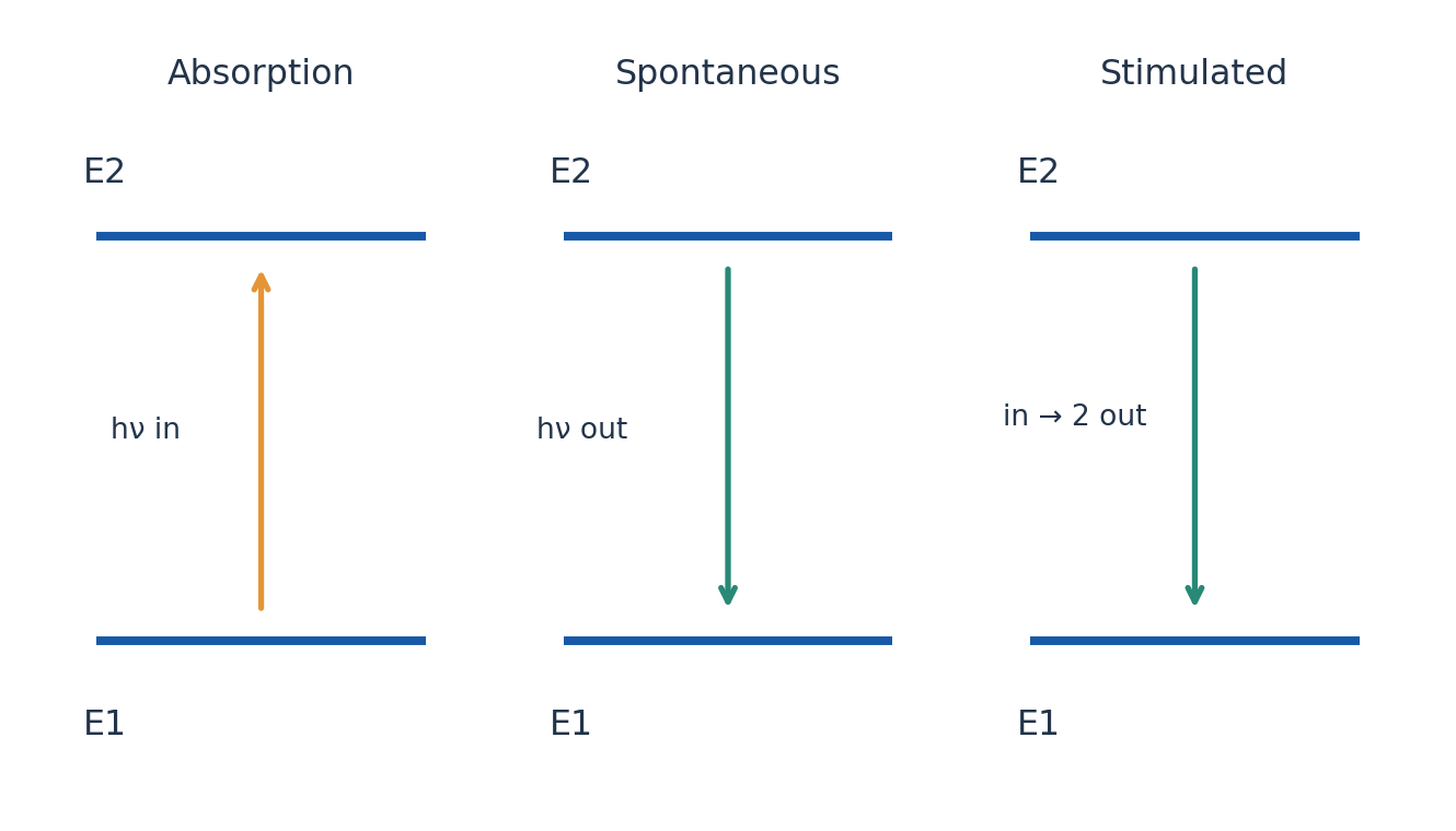
The stimulated photon shares the relevant optical mode properties, including frequency, direction and phase relation in the ideal single-mode description. Statements that every real laser has exactly one wavelength or perfect coherence are too strong: linewidth, modes and stability depend on the system.
Population inversion refers to a non-equilibrium population balance capable of net gain. For equal level degeneracies the elementary condition is N2 > N1; with unequal degeneracies compare N2/g2 with N1/g1. Pumping supplies energy to maintain this distribution against relaxation.
Worked Problem 4.9: Photon Energy from Level Spacing
Problem: A transition emits at 632.8 nm. Find photon energy in joules and eV.
Method: E = hc/λ.
Calculation: Convert wavelength to 632.8 × 10^-9 m, then divide joules by e for eV.
Answer: E = 3.13914 × 10^-19 J = 1.95930 eV.
Check: Transition energy depends on wavelength, not on beam power.
7. CSE and BT: Einstein Coefficients and Equilibrium
With spectral radiation energy density uν per unit frequency, absorption rate is N1B12uν, stimulated-emission rate is N2B21uν and spontaneous-emission rate is N2A21. A has units inverse time. The B units depend on the chosen spectral-energy-density convention, which must accompany a numerical ratio.
At thermal equilibrium, upward and downward transition rates balance. Combine N1B12uν = N2A21 + N2B21uν with the equilibrium population ratio and Planck’s radiation law. The comparison gives g1B12 = g2B21 and A21/B21 = 8πhν³/c³ for the vacuum spectral-frequency convention.
For equal degeneracies the absorption and stimulated coefficients are equal. The spontaneous-to-stimulated rate ratio for one excited atom is A21/(B21uν), not A21/B21 alone. The latter has the dimensions of spectral energy density and grows as ν³.
Thermal equilibrium does not provide the inversion needed by an ordinary positive-temperature laser. A pumped multilevel system and metastable storage create a non-equilibrium route. TX needs the interactions and laser components; this explicit coefficient analysis is the CSE/BT depth.
Worked Problem 4.10: Einstein Coefficient Ratio
Problem: Evaluate A21/B21 for 694.3 nm using vacuum spectral energy density per unit frequency.
Method: A21/B21 = 8πhν³/c³ = 8πh/λ³.
Calculation: Use λ in metres and the stated spectral-frequency convention.
Answer: A21/B21 = 4.9757 × 10^-14 J s/m³.
Check: The ratio is dimensional. Divide it by uν to obtain the spontaneous-to-stimulated rate ratio.
Worked Problem 4.11: Degeneracy and Gain Condition
Problem: Let g1 = 2, g2 = 4, N1 = 3.0 × 10^18 and N2 = 5.0 × 10^18 m^-3. Does N2 > N1 alone establish gain? Find B12/B21.
Method: Gain requires N2/g2 > N1/g1; g1B12 = g2B21.
Calculation: N2/g2 = 1.25 × 10^18; N1/g1 = 1.50 × 10^18.
Answer: No net inversion by this criterion; B12/B21 = 2.
Check: Ignoring degeneracy would give the wrong conclusion even though the upper population is larger.
8. Laser System: Pumping, Cavity and Output
A laser needs an active gain medium, a pumping mechanism and appropriate optical feedback or equivalent resonant structure. In the standard linear resonator a highly reflecting mirror and a partly transmitting output coupler return light through the medium while allowing a useful beam to leave.
A metastable upper level can hold population long enough for pumping to build gain. Rapid depletion of a lower laser level can help maintain inversion. A simple isolated two-level system cannot sustain ordinary inversion by resonant pumping alone because absorption and stimulated emission compete.
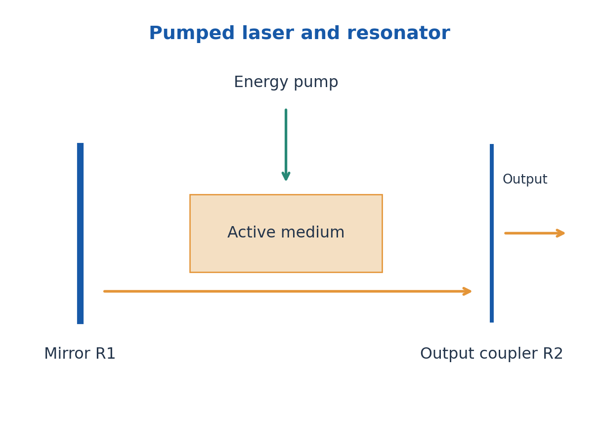
Using intensity gain g and distributed intensity loss α, a round trip of a cavity length L multiplies intensity by R1R2 exp[2(g – α)L]. Threshold occurs when that factor equals one, giving gth = α + ln[1/(R1R2)]/(2L). The mirrors use intensity reflectivities in this convention.
Above threshold saturation and dynamics determine the actual output; the unsaturated exponential expression does not predict unlimited power. Directionality, spectral width and coherence are useful laser features with finite practical values. Pump light, electrical discharge and output light must be distinguished in the diagram.
Worked Problem 4.12: Laser Threshold Gain
Problem: A cavity has L = 0.25 m, R1 = 0.98, R2 = 0.90 and intensity loss α = 0.080 m^-1. Find threshold intensity gain g.
Method: gth = α + ln[1/(R1R2)]/(2L).
Calculation: The reflectivity product is 0.882 and the round-trip distance is 0.50 m.
Answer: gth = 0.33113 m^-1.
Check: This uses intensity reflectivities and intensity gain/loss coefficients throughout.
9. Ruby Laser: Construction and Three-Level Operation
Ruby is chromium-doped aluminium oxide. Cr3+ ions supply the active optical levels while the host supports the solid medium. A flash lamp optically pumps ions into higher absorption bands; rapid non-radiative relaxation transfers population to a comparatively long-lived metastable level.
The useful stimulated transition is near 694.3 nm in the red. Its lower level belongs to the ground manifold, making ruby a three-level laser. Substantial ground-state depletion is needed for inversion, so the introductory ruby system has a relatively high pumping requirement and normally gives pulsed output.
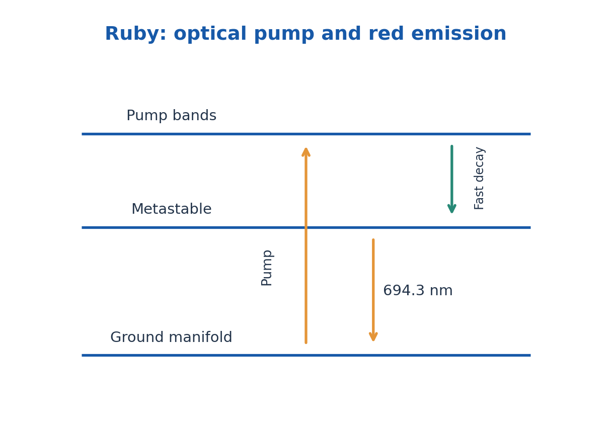
The rod ends or external mirrors form a resonator and an output coupler releases part of the amplified light. A flash-lamp pulse is not identical to the generated coherent optical pulse; energy transfer, losses and storage determine their relationship.
In an exam draw pump arrows upward, a fast non-radiative path into the metastable level and the laser transition downward. Label the active ion, host, pump and wavelength. Do not label the pump absorption as the 694.3 nm output.
Worked Problem 4.13: Ruby Pulse Photon Count
Problem: A ruby pulse has energy 0.050 J at 694.3 nm. Estimate emitted photon count.
Method: Nph = pulse energy/(hc/λ).
Calculation: Compute the energy per photon, then divide 0.050 J by it.
Answer: Nph ≈ 1.7476 × 10^17.
Check: This is an emitted-pulse estimate; pump-energy consumption would require an efficiency model.
10. He-Ne Laser: Discharge Pumping and Energy Transfer
A He-Ne laser uses a low-pressure helium-neon mixture excited by an electrical discharge. Electron collisions excite helium into metastable states. Collisions then transfer energy efficiently to suitable near-resonant excited neon states, building the population for a neon laser transition.
The familiar red output is at 632.8 nm. Neon emits this laser line; helium is primarily the energy-transfer partner. Fast relaxation from lower levels and continuing discharge pumping support continuous operation in the common laboratory arrangement.
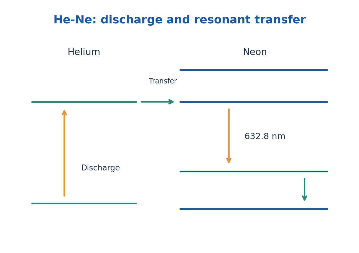
A resonator selects useful transitions among the available neon lines. The simplified energy-level picture is a multilevel arrangement, commonly represented by four effective levels. It should show helium excitation, transfer to neon, stimulated emission and lower-level depopulation.
Compare ruby and He-Ne by medium, pump, level structure, wavelength and operating mode. They share stimulated emission and feedback, but one is an optically pumped solid-state three-level system and the other is a discharge-pumped gas system with interspecies energy transfer.
Worked Problem 4.14: He-Ne Photon Rate
Problem: A 632.8 nm He-Ne beam has power 1.5 mW. Find photon rate.
Method: Rate = Pλ/(hc).
Calculation: Use P = 1.5 × 10^-3 J/s.
Answer: Rate = 4.7784 × 10^15 photons/s.
Check: The output line comes from neon, while helium transfers excitation energy.
11. Photonics Applications and Textile-Specific Selection
Optical fibres carry information in communication links and can deliver or collect light in sensing instruments. Laser alignment and ranging use directionality and stable optical referencing; spectroscopy uses a selected spectral interaction. A useful application explanation names the measured variable, optical interaction and detector output.
CSE examples include fibre data links and optical interconnect concepts. BT examples include fluorescence excitation, optical analysis and fibre-based observation. A laser source is only one component; wavelength selectivity, sample interaction, optics and detector calibration complete the instrument.
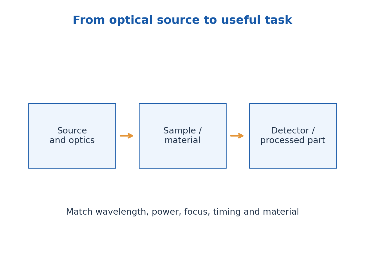
TX-prescribed applications: Laser cutting and engraving localise optical energy in suitable fabric, while alignment and inspection use optical measurement. Material absorption, wavelength, power, spot size, scanning speed and heat-affected zone determine the result. A laser that cuts one textile well may damage or poorly couple into another.
Fibres can be used for illumination, sensing or communication in textile systems. Match bend tolerance, optical response, durability and connector design to the application. Optical loss and source ageing are practical engineering considerations, not proof that every ideal ray model has failed.
Worked Problem 4.15: Pulse Average and Repetition Power
Problem: A laser produces 4.0 mJ pulses of rectangular 20 ns duration at 200 pulses/s. Find within-pulse power and long-time average.
Method: Ppulse = Epulse/Δt; Paverage = Epulse frep.
Calculation: 4.0 mJ = 0.0040 J; 20 ns = 20 × 10^-9 s.
Answer: Within-pulse power = 200 kW; long-time average = 0.800 W.
Check: The large pulse power is not the continuous average. Nonrectangular pulses need the stated temporal shape.
12. B. Ultrasonics: Wave Properties and Resonance – TX
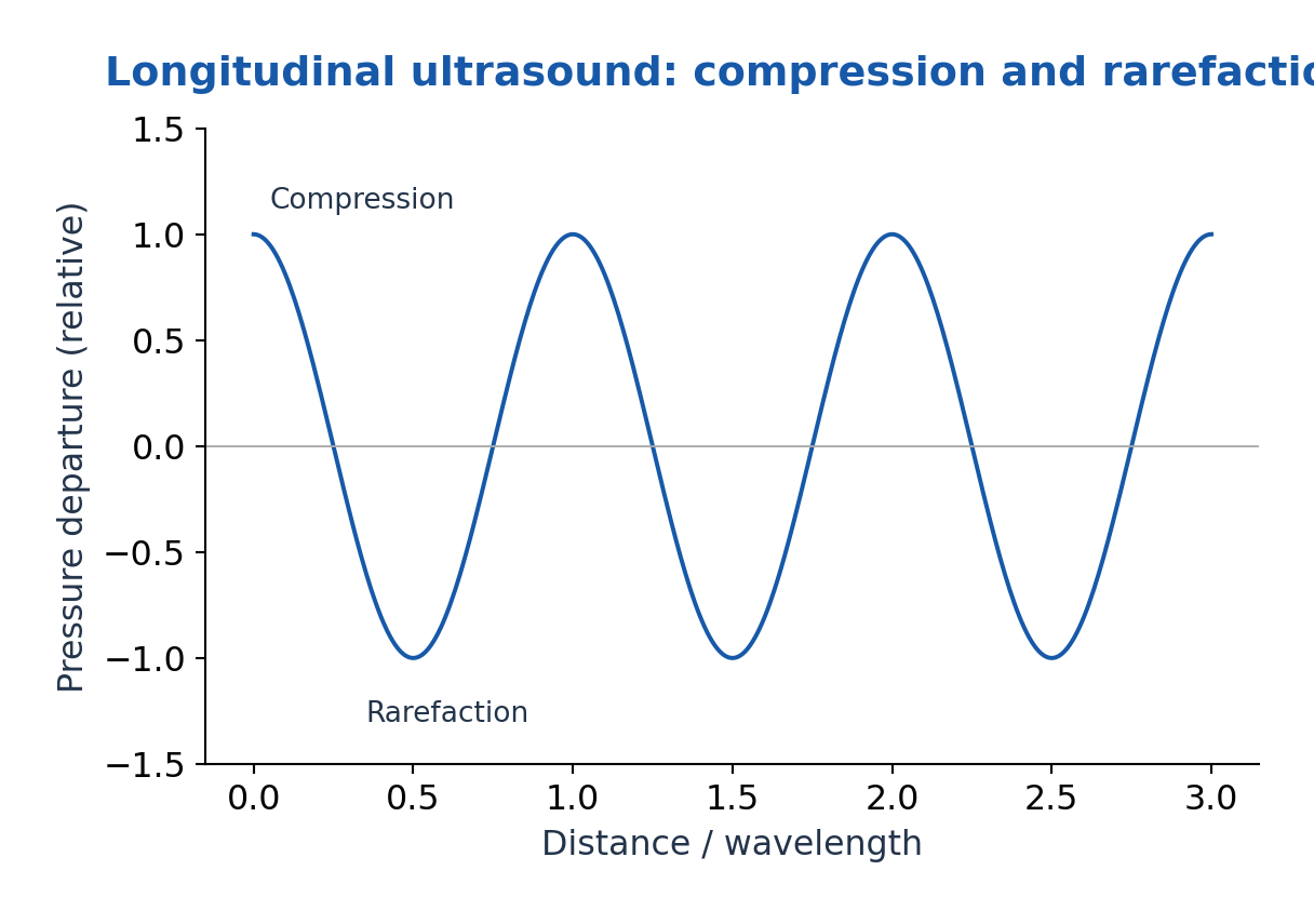
Ultrasound is sound above the conventional upper audible range, roughly 20 kHz for a typical introductory boundary. It is a mechanical wave requiring a medium. In fluids it propagates mainly as longitudinal pressure waves; solids can support longitudinal and shear waves depending on geometry and excitation.
Frequency f, wavelength λ and phase speed v satisfy v = fλ for the specified wave mode and medium. Acoustic impedance for a simple plane longitudinal wave is Z = ρv. At an ideal normal boundary the reflected intensity fraction is [(Z2 – Z1)/(Z2 + Z1)]² when losses and mode conversion are neglected.
A driven elastic element responds strongly near its natural resonance. The useful resonant frequency depends on material stiffness, density, dimensions and boundary conditions. Coupling the element to liquid or other loads can shift resonance and add damping; a free-element estimate is not an exact loaded-system value.
Ultrasonic processes can produce acoustic streaming, heating and cavitation under appropriate conditions. Cavitation involves bubble growth and collapse in liquid and can assist cleaning, but it is not a universal property of every weak ultrasound signal. Separate a measurement pulse from a high-power processing field.
Worked Problem 4.16: Ultrasonic Wavelength
Problem: A 2.0 MHz longitudinal wave travels at 1500 m/s in a liquid. Find λ.
Method: λ = v/f.
Calculation: Use f = 2.0 × 10^6 Hz.
Answer: λ = 0.750 mm.
Check: Ultrasound is mechanical, so use the sound speed of the liquid, not c.
Worked Problem 4.17: Acoustic Impedance Mismatch
Problem: A liquid has ρ = 1000 kg/m³ and v = 1500 m/s; a second medium has ρ = 2500 and v = 5000 in matching SI units. Find normal reflected-intensity fraction.
Method: Z = ρv; Rint = [(Z2 – Z1)/(Z2 + Z1)]².
Calculation: Z1 = 1.50 × 10^6; Z2 = 1.25 × 10^7 kg/(m² s).
Answer: Reflected fraction = 0.61735, or 61.735%.
Check: This ideal boundary result neglects absorption, mode conversion and oblique incidence.
13. Magnetostriction Generation of Ultrasound – TX
Magnetostriction is the change of a suitable ferromagnetic rod’s dimensions when its magnetic state changes. A coil driven by an alternating current creates an alternating magnetising field; the rod can then execute longitudinal vibration and transfer acoustic energy to a coupled medium.
A practical oscillator has an electronic drive and feedback or a controlled frequency source, a magnetising coil, a rod and a coupling arrangement. Tune the drive to a mechanical resonance. For the ideal slender free-free rod fundamental longitudinal mode, f ≈ (1/2L)√(Y/ρ); other supports and loads change the frequency.
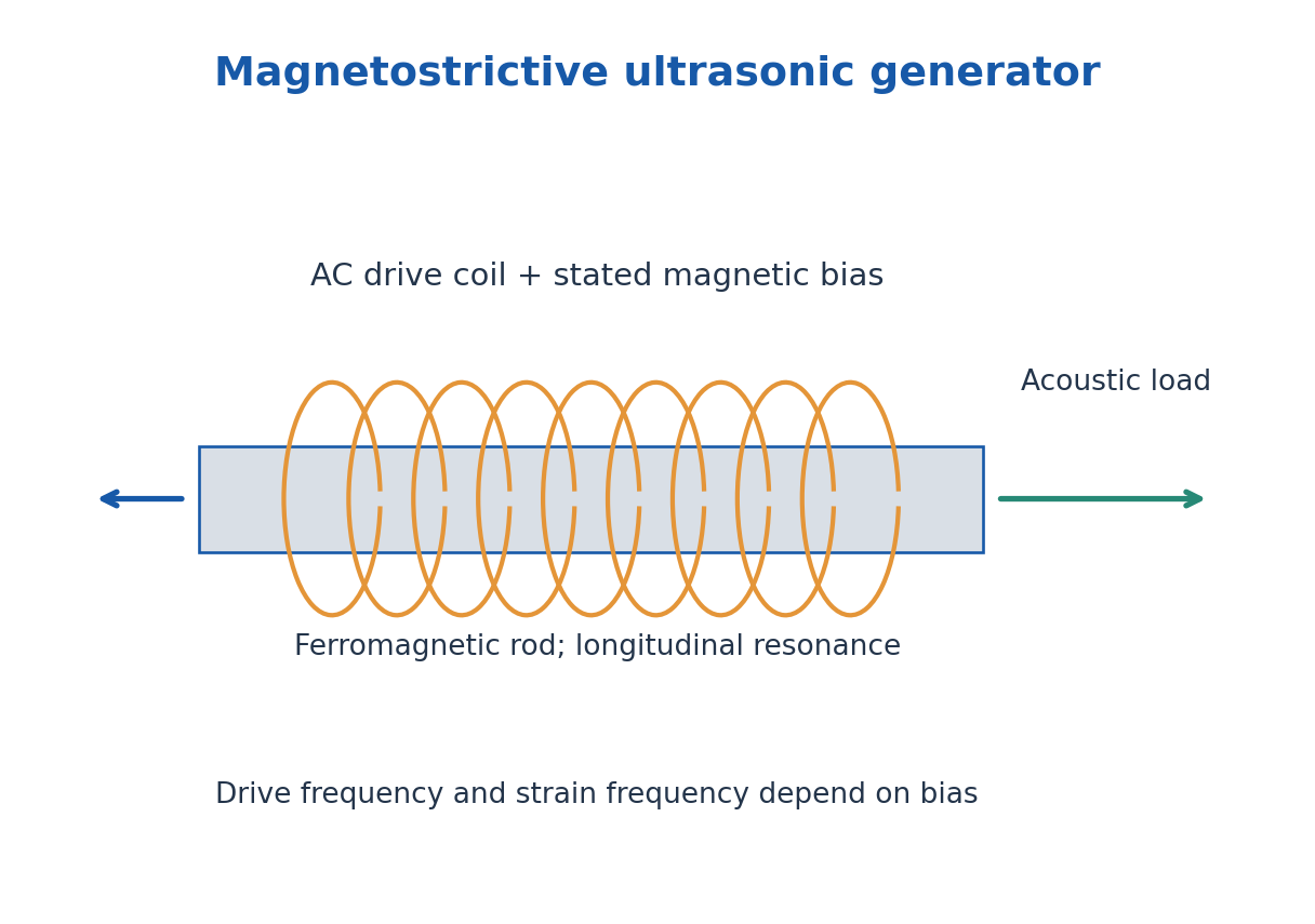
Because magnetostrictive strain can be approximately even in field near zero bias, an unbiased sinusoidal field may generate a strong strain component at twice the electrical drive frequency. A DC magnetic bias can provide a useful nearly linear response around its operating point. State the bias and frequency convention rather than equating all frequencies automatically.
Advantages include a robust mechanical drive; limitations include magnetic and eddy-current losses, restricted high-frequency response and material heating. The coil is not the emitted sound wave. In a labelled diagram keep the drive circuit, magnetic field, mechanical vibration and acoustic output separate.
Worked Problem 4.18: Longitudinal Rod Resonance
Problem: Estimate the fundamental free-free rod frequency for L = 0.100 m, Y = 200 GPa and ρ = 8000 kg/m³.
Method: f ≈ √(Y/ρ)/(2L).
Calculation: Elastic-wave speed estimate = 5000 m/s.
Answer: f ≈ 25.0 kHz.
Check: Actual supports, magnetic state and acoustic loading can shift the mechanical resonance.
Worked Problem 4.19: Unbiased Strain Harmonic
Problem: An unbiased sinusoidal magnetising field is at 15 kHz, and small-field strain follows λmag ∝ H². Find the non-DC strain frequency.
Method: cos²ωt = [1 + cos(2ωt)]/2.
Calculation: The squared sinusoid has a DC term and a term at twice drive frequency.
Answer: Non-DC strain component is at 30 kHz.
Check: DC bias changes the small-signal response; do not automatically double frequency in every magnetostrictive oscillator.
14. Piezoelectric Generation and Resonance – TX
The converse piezoelectric effect produces mechanical strain when an electric field is applied to a suitable crystal or poled ceramic. Electrodes across a plate supply an alternating field; near mechanical resonance the plate can emit a strong ultrasonic wave into the coupled load.
For an ideal thickness-mode plate, a simple estimate is f ≈ vt/(2t), where vt is the relevant longitudinal elastic-wave speed and t is plate thickness. The mode, electrical boundary, material constants and loading determine the precise resonance and antiresonance. Do not use an arbitrary bulk speed without specifying the intended mode.
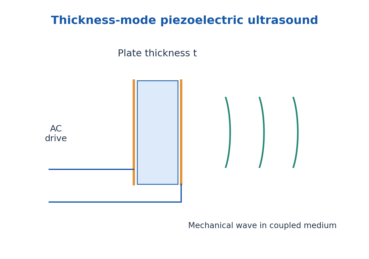
The direct effect converts received mechanical stress to electric charge, allowing the same physical element or a separate receiver to detect an echo. Electronics normally include a pulse or oscillator source, matching/drive stage, transducer, receiver amplification and timing or amplitude measurement.
Quartz is a familiar piezoelectric example; suitable ceramics can provide strong electromechanical coupling after poling. Not every dielectric is piezoelectric. Good mechanical coupling, electrode integrity and appropriate damping matter as well as the quoted frequency.
Worked Problem 4.20: Thickness-Mode Plate
Problem: A piezoelectric plate uses relevant longitudinal speed 4000 m/s. Find thickness for an ideal 2.0 MHz fundamental thickness resonance.
Method: t ≈ v/(2f).
Calculation: t = 4000/(2 × 2.0 × 10^6).
Answer: t ≈ 1.00 mm.
Check: Use the stated mode speed; an arbitrary transverse speed or loaded resonance requires a different model.
15. Ultrasound Detection and Textile Applications – TX
Piezoelectric receivers convert pressure-induced stress to an electrical signal. A hydrophone is an appropriately designed sound-pressure receiver for a fluid. Other demonstrations use thermal effects or diffraction of light by a periodic acoustic-density pattern; each detects a different consequence of the mechanical wave.
In pulse-echo measurement a pulse travels to an interface and back. With round-trip time Δt and known mode speed v, depth is d = vΔt/2. The factor two is essential. Through-transmission uses a separate receiver and a one-way travel path. Couplant reduces an unwanted air gap, whose impedance mismatch can otherwise reflect much of the signal.
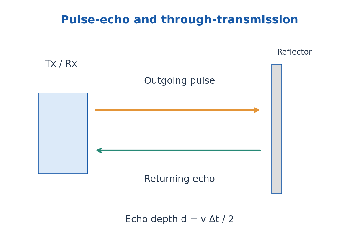
Textile applications include ultrasonic-assisted cleaning or wet processing, inspection, and bonding or cutting of suitable thermoplastic materials. Mechanical vibration and local heat can support welding at contact regions. Choice of fibre type, frequency, pressure, amplitude and dwell time controls the outcome.
An application answer should connect generation, coupling, interaction, detection or processing result and limitations. A strong echo can indicate an interface but its amplitude also depends on coupling, attenuation and geometry; it does not alone identify a unique defect size or material composition.
Worked Problem 4.21: Pulse-Echo Depth
Problem: An echo returns after 80 microseconds in a medium with speed 1500 m/s. Estimate reflector depth.
Method: d = vΔt/2 for a round trip.
Calculation: d = 1500 × 80 × 10^-6 / 2.
Answer: Depth = 0.0600 m = 60.0 mm.
Check: Without the half factor the calculation gives the full travelled path, not depth.
Worked Problem 4.22: Ultrasonic Intensity Loss
Problem: A stated intensity attenuation coefficient is 4.0 m^-1 over a one-way 0.10 m path. Find remaining fraction; for an ideal echo over the same depth find the propagation-only round-trip fraction.
Method: Intensity fraction = exp(-αIL); round-trip path is 2L.
Calculation: One-way exponent is -0.4; return-path exponent is -0.8.
Answer: One-way = 0.67032; round-trip = 0.44933.
Check: This explicitly uses an intensity coefficient and excludes reflection and transducer conversion losses.
16. C. Dielectric Vectors and Susceptibility – EE and ECE
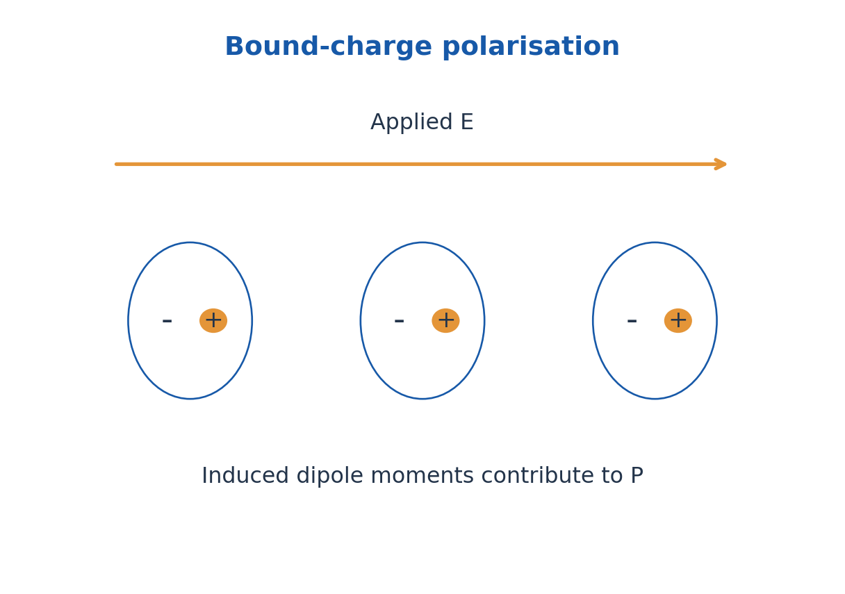
A dielectric responds to an applied electric field mainly through bound-charge displacement and orientation rather than large steady free-current flow. Polarisation P is electric dipole moment per unit volume, in C/m². The macroscopic displacement is D = ε0E + P and Gauss’ law uses ∇·D = ρfree.
For a linear isotropic dielectric, P = ε0χe E, ε = ε0(1 + χe) and relative permittivity εr = 1 + χe. Susceptibility is dimensionless. These simple scalar relations do not describe every anisotropic, nonlinear or frequency-dependent material.
A parallel-plate capacitor of area A and separation d has C = εA/d when fringe effects are negligible. Filling the gap with a suitable dielectric increases capacitance. At fixed voltage its stored energy rises because the source supplies charge; for a disconnected capacitor with fixed charge the energy falls. State the electrical constraint.
Useful properties include permittivity, dielectric strength, loss and stability. A high dielectric constant does not automatically mean low loss or high breakdown strength. Capacitors, insulation and sensing applications require different compromises.
Worked Problem 4.23: D, P and Susceptibility
Problem: A linear dielectric has εr = 6 and E = 1.0 × 10^5 V/m. Find χe, P and D.
Method: χe = εr – 1; P = ε0χeE; D = ε0εrE.
Calculation: χe = 5; multiply ε0E by five and six.
Answer: P = 4.4271 × 10^-6 C/m²; D = 5.3125 × 10^-6 C/m²; χe = 5.
Check: D – P must equal ε0E.
Worked Problem 4.24: Capacitance and Charge
Problem: A dielectric capacitor has εr = 4, A = 0.015 m², d = 0.50 mm and V = 50 V. Find C and Q, neglecting fringing.
Method: C = ε0εrA/d; Q = CV.
Calculation: Convert d to 5.0 × 10^-4 m.
Answer: C = 1.06250 nF; Q = 53.12513 nC.
Check: Area is in m² and the field geometry is assumed uniform.
Worked Problem 4.25: Energy After Disconnected Dielectric Insertion
Problem: A capacitor initially stores 12 microJ and is disconnected. A dielectric increases its capacitance by factor four with charge fixed. Find final energy.
Method: At fixed Q, U = Q²/(2C).
Calculation: The energy is inversely proportional to capacitance.
Answer: Final energy = 3.0 microJ.
Check: At fixed voltage the energy would increase instead, with energy supplied by the source.
17. Polarisation Mechanisms and Frequency Response
Electronic polarisation shifts the electron cloud relative to the nucleus. Ionic polarisation displaces positive and negative sublattices in ionic materials. Orientation polarisation aligns permanent dipoles against thermal disorder. Space-charge or interfacial polarisation results from charge accumulation at interfaces or in heterogeneous structures.
The mechanisms respond on different timescales. As field frequency rises, slower mechanisms can no longer follow the oscillation effectively, changing the real permittivity and dissipative loss. Orientation contributions generally weaken with increasing temperature in simple dilute-dipole models because thermal agitation opposes alignment.
If an individual induced dipole is p = αaE and interactions are neglected, P ≈ NαaE. The molecular polarizability αa has units C m²/V; it is not the same as dimensionless bulk susceptibility. Dense materials require a local-field model before connecting the two accurately.
Dielectric materials are used in capacitors, electrical insulation, substrates and sensors. In biotechnology, dielectric measurements can probe hydration and material response, but observed signals depend on geometry, frequency and conduction as well as polarisation. Select an operating frequency and calibration rather than assigning a specimen one universal dielectric value.
18. Dielectric Applications, Loss and Breakdown
A capacitor dielectric increases capacitance through its polarisation response. Insulation must also resist leakage and breakdown. Substrates need stable geometry and suitable dielectric loss over the operating frequency. These requirements make dielectric constant, loss, conductivity and strength separate selection properties.
Under a sinusoidal field, complex relative permittivity can be written εr* = εr′ – iεr″ with an exp(iωt) convention. The real part describes the in-phase storage response and the imaginary part the associated loss convention. The loss tangent is tanδ = εr″/εr′ under that convention.
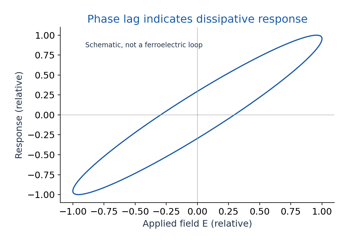
For a simple lossy capacitor driven by rms voltage Vrms, dielectric-loss power is approximately ωC Vrms² tanδ using the stated equivalent small-loss model. The capacitance and loss tangent should apply at the operating frequency and temperature. The DC leakage term may need separate treatment depending on how loss is defined.
Breakdown occurs when the material or assembly cannot sustain the applied field. A uniform-field estimate is E ≈ V/d, but edges, voids, humidity and defects can concentrate the local field. Increasing permittivity does not guarantee a larger breakdown voltage. Use stated model data for numerical exercises rather than inventing a universal strength.
Worked Problem 4.26: Small-Loss Capacitor Heating
Problem: A 2.0 nF capacitor at 10 kHz has tanδ = 0.020 and Vrms = 100 V. Estimate dielectric-loss power in the stated small-loss model.
Method: Ploss ≈ ωC Vrms² tanδ.
Calculation: ω = 2π × 10^4 rad/s; use rms voltage.
Answer: Ploss ≈ 0.025133 W.
Check: Using a peak voltage in the rms formula would introduce a factor-two error.
Worked Problem 4.27: Uniform Breakdown Estimate
Problem: A model dielectric strength is 12 MV/m. Estimate the uniform-field voltage limit across 0.80 mm thickness.
Method: V ≈ Emax d.
Calculation: Use Emax = 12 × 10^6 V/m and d = 8.0 × 10^-4 m.
Answer: Estimated limit = 9.6 kV.
Check: This is not a practical safety rating; edges, defects and environment can change local breakdown.
19. Magnetic Classes, Susceptibility and Domains
Magnetisation M is magnetic dipole moment per volume, in A/m. The macroscopic relation is B = μ0(H + M). In a weak linear isotropic response, M = χmH and μr = 1 + χm. Magnetic susceptibility χm is dimensionless; permeability has different units.
Diamagnets have a small negative susceptibility in the simple static description and tend to oppose applied field. Paramagnets have small positive susceptibility associated with permanent moments tending to align. Ferromagnets show cooperative ordering, domains, strong nonlinear response and hysteresis below the relevant transition temperature.
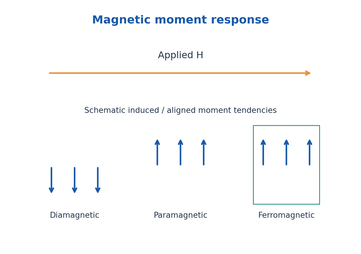
In a simple paramagnetic regime, Curie’s law gives χm = C/T with absolute temperature T. It is not a general law for every temperature, field or material. Ferromagnetic ordering disappears above a Curie temperature, where an appropriate paramagnetic description becomes necessary.
Domain-wall movement and moment rotation explain much of ferromagnetic magnetisation. A domain is a region of aligned moments, not a separate lump of electric charge. Soft magnetic materials are useful when magnetisation must reverse with low loss; hard magnetic materials retain strong magnetisation for permanent-magnet applications.
| Type | Ideal Weak-Field Trend |
|---|---|
| Diamagnetic | Small χm < 0; induced opposition |
| Paramagnetic | Small χm > 0; thermal competition |
| Ferromagnetic | Domains, nonlinearity and hysteresis |
Worked Problem 4.28: Magnetisation and Relative Permeability
Problem: A weak linear material has χm = 0.005 and H = 800 A/m. Find M, μr and B.
Method: M = χmH; μr = 1 + χm; B = μ0(H + M).
Calculation: M = 4.0 A/m; H + M = 804 A/m.
Answer: M = 4.0 A/m; μr = 1.005; B = 0.00101034 T.
Check: A full ferromagnetic loop cannot generally be replaced by one constant χm.
Worked Problem 4.29: Curie-Law Temperature Change
Problem: A suitable paramagnet has χm = 0.0040 at 300 K. Assuming χm = C/T over the interval, find χm at 450 K.
Method: χ2/χ1 = T1/T2.
Calculation: χ2 = 0.0040 × 300/450.
Answer: χm(450 K) = 0.002667 approximately.
Check: Use kelvin and the explicitly stated Curie-law range.
20. Hysteresis Loop, Coercivity, Remanence and Loss
When a ferromagnet is driven through a cycle, its response depends on previous magnetisation. In a B-H loop, remanent flux density Br is the remaining B when H returns to zero after magnetisation. Coercive field Hc is the reverse H needed to bring B to zero on the specified loop.
Saturation describes the approach to maximum alignment under strong field. Remanence, coercivity and saturation are distinct. A narrow loop generally indicates lower hysteresis loss and easier reversal, while a wide loop indicates greater resistance to demagnetisation. Measurement definitions and material conditions should be stated.
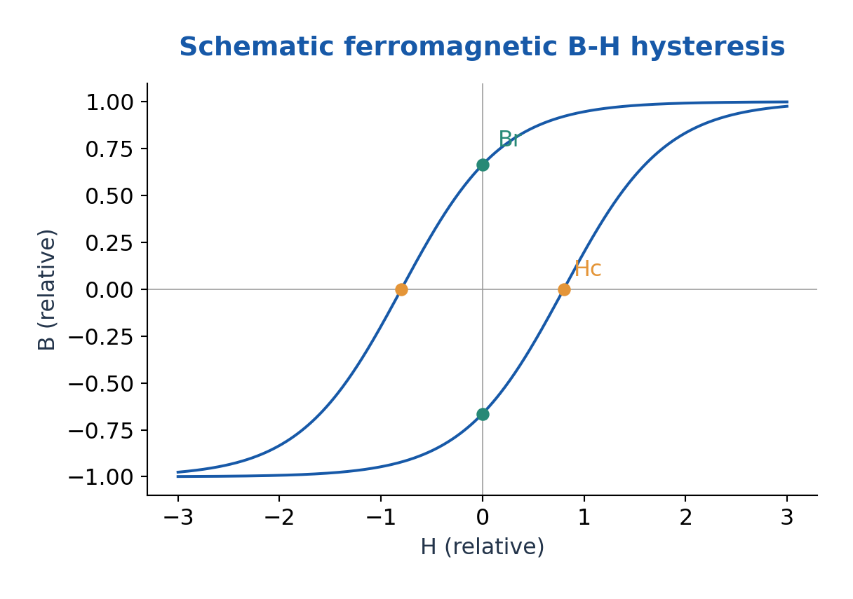
For quasistatic cyclic operation, hysteresis energy dissipated per volume per cycle is the magnitude of the loop area ∮H dB, in J/m³. Multiply by frequency and core volume to estimate hysteresis power under the stated assumption that loop area is unchanged. Eddy-current and other dynamic losses are additional.
Applications include transformer and motor cores, permanent magnets and magnetic recording. Reducing hysteresis loss is valuable for frequently reversing cores; high coercivity is valuable for magnets resisting accidental demagnetisation. A permanent magnet and an efficient AC core therefore need different properties.
Worked Problem 4.30: Hysteresis Energy and Power
Problem: A loop encloses 180 J/m³ per cycle. Core volume is 2.0 × 10^-4 m³ and cycle frequency is 60 Hz. Find energy per cycle and hysteresis power.
Method: Energy = loop area × volume; power = energy × frequency.
Calculation: Energy = 180 × 2 × 10^-4 = 0.036 J.
Answer: Energy per cycle = 0.036 J; hysteresis power = 2.16 W.
Check: Additional eddy-current loss is not contained in this fixed-area quasistatic estimate.
21. Magnetic Material Selection and Applications
Soft magnetic materials are magnetised and demagnetised comparatively easily. Low coercivity and a narrow appropriate loop help reduce loss in AC cores. Hard magnetic materials resist demagnetisation and are useful for permanent magnets. The labels do not refer directly to mechanical hardness.
Transformer and motor cores also need suitable saturation flux density, frequency response, resistivity and manufacturability. Thin insulated laminations reduce eddy-current loops in appropriate metallic cores; high-resistivity ferrites can be useful at higher frequencies. Hysteresis loss and eddy-current loss have different origins.
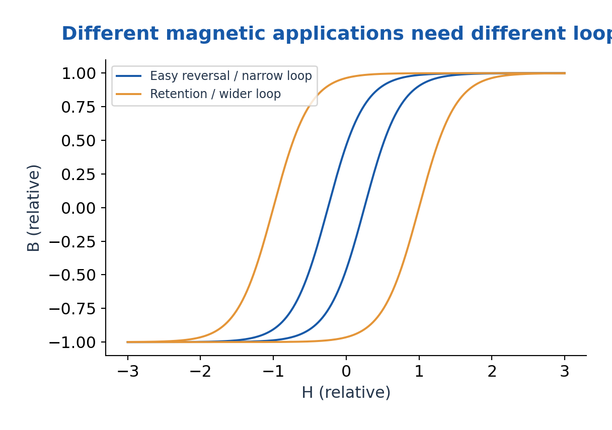
A magnetic sensor can convert a field or magnetisation change into another measurable signal, while an actuator uses magnetic forces to cause motion. Hysteresis can be useful for memory and retention but inconvenient for a reversible accurate sensor. The preferred loop therefore depends on the task.
An engineering comparison should specify operating field, frequency, temperature, allowable loss and required retention. A material with a large relative permeability in one weak-field test need not retain that value near saturation or at another frequency. Treat nonlinear loops and linear susceptibility models as different descriptions.
22. D. Band Theory and Electrical Material Classes – ME
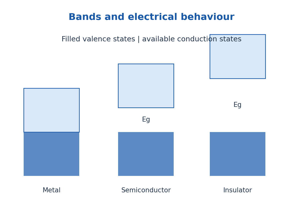
In a crystal, interacting atomic states form energy bands separated by forbidden gaps. Electrical conduction depends on allowed states, their occupation and carrier mobility. A partially filled band or suitable band overlap supports metallic conduction, while a full band alone cannot carry ordinary small-field net current in the ideal picture.
A semiconductor has accessible thermal or optical excitation across a gap from valence to conduction states. Excitation creates an electron and a valence hole. An insulator has a much less accessible excitation gap under ordinary operating conditions. There is no one temperature-independent numerical gap boundary that perfectly separates the categories.
Intrinsic semiconductors have equilibrium n = p. Doping supplies donors or acceptors that shift the majority-carrier balance. Conductivity is σ = e(nμn + pμp), and resistivity is its reciprocal. For metals, temperature commonly increases scattering; for intrinsic semiconductors, thermally activated carriers can dominate the temperature response.
Mechanical systems combine conductors for current paths, semiconductors for control or sensing and insulators for isolation. Temperature, contact resistance, vibration and material strain affect practical behaviour. Band classification supplies the electronic foundation but does not by itself determine every property of a finished component.
Worked Problem 4.31: One-Carrier Conduction
Problem: A material has n = 5.0 × 10^21 m^-3 and μ = 0.080 m²/(V s). Find σ and resistivity.
Method: σ = neμ; ρel = 1/σ.
Calculation: Multiply concentration, charge magnitude and mobility, then invert.
Answer: σ = 64.08707 S/m; ρel = 0.015604 ohm m.
Check: This model assumes a dominant carrier and ignores contact resistance.
23. ME: Dielectric, Piezoelectric and Ferroelectric Response
ME also requires dielectric materials: use D = ε0E + P to distinguish applied field, bound-charge response and free-charge flux. For a linear isotropic material P = ε0χeE and εr = 1 + χe. A dielectric stores field energy but real materials can also have conduction and polarisation loss.
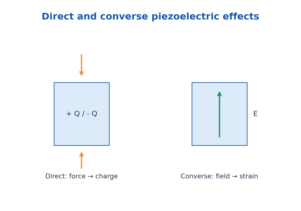
The direct piezoelectric effect is electric polarisation produced by suitable mechanical stress. The converse effect is mechanical strain produced by an applied field. It requires an appropriate non-centrosymmetric crystal symmetry; not every dielectric is piezoelectric. In a simplified one-dimensional sensor model, charge Q = dF with d in C/N.
Ferroelectric materials possess a spontaneous polarisation that can be switched by an applied electric field. Their P-E response can exhibit hysteresis, with remanent polarisation and coercive field. Ferroelectricity is not a requirement for iron atoms, and a permanent electric dipole alone does not prove switchable ferroelectric order.
Ferroelectric materials are piezoelectric in their polar phase, but many piezoelectrics are not ferroelectric. Applications include pressure and vibration sensors, actuators, ultrasonic transducers, capacitors and non-volatile memory. A mechanical sensor or actuator must transfer the intended stress without shorting or damaging the active layer.
Worked Problem 4.32: Piezoelectric Charge Readout
Problem: An ideal sensor has d = 200 pC/N, force 25 N and capacitance 1.0 nF. Estimate Q and open-circuit voltage.
Method: Q = dF; V = Q/C.
Calculation: Q = 200 × 10^-12 × 25 = 5.0 × 10^-9 C.
Answer: Q = 5.0 nC; V = 5.0 V.
Check: Leakage and measurement loading can reduce or change the observed time-dependent voltage.
24. Hall Effect: Transverse Force and Carrier Sign – ME
A current-carrying specimen in a perpendicular magnetic field can develop a transverse electric field because carriers are deflected sideways by the magnetic Lorentz force. Accumulated charge creates a balancing Hall field. The sign reveals carrier behaviour only with a declared axis, contact and polarity convention.
Choose conventional current density Jx along +x and magnetic field Bz along +z. Define RH = Ey/(JxBz). In a simple one-carrier isotropic Drude model RH = 1/(nq), where q is signed carrier charge. Thus electrons give RH = -1/(ne) and holes RH = +1/(pe) in this convention.
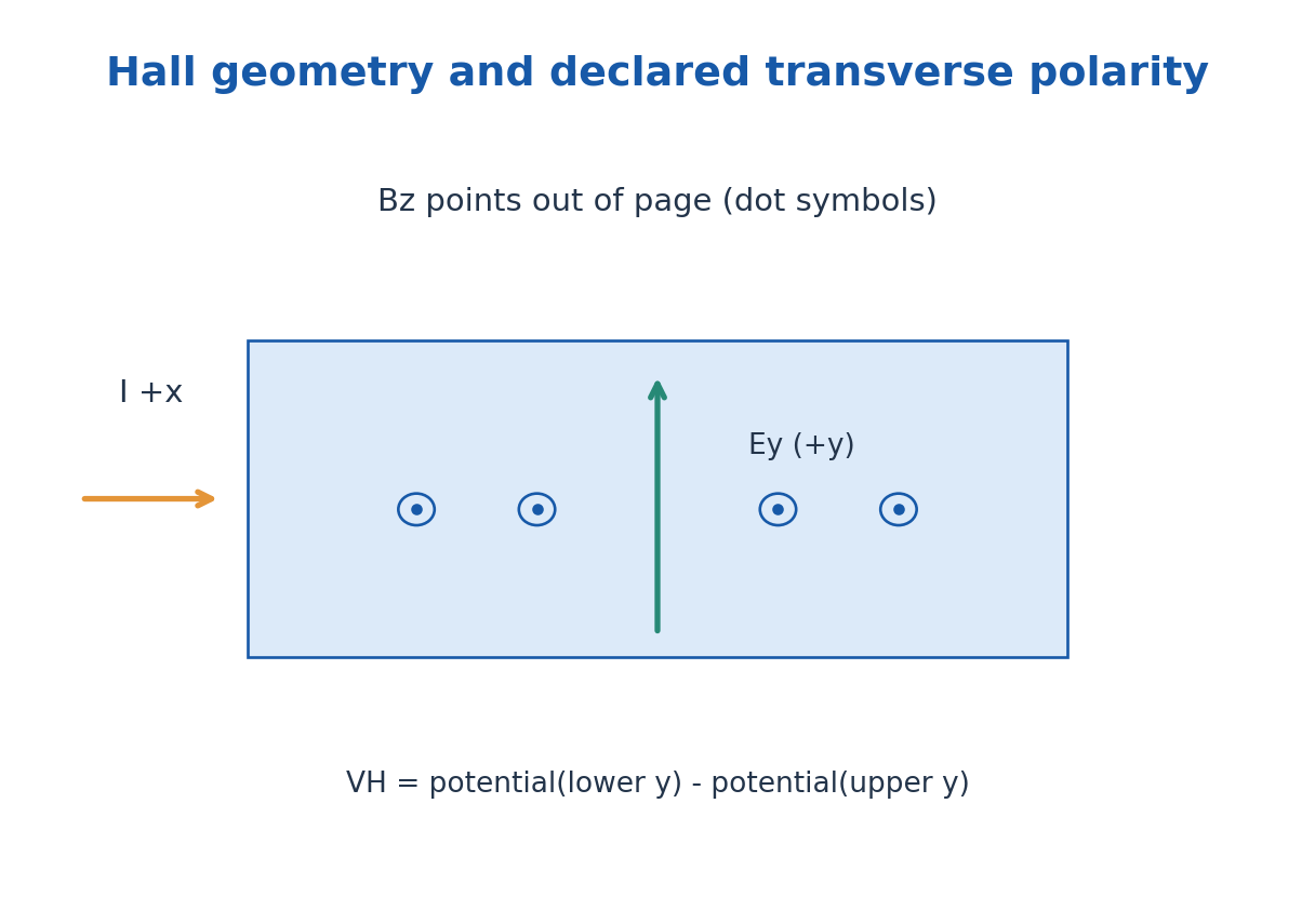
For a slab of width w in y and thickness t in z, Jx = I/(wt). Define the reported Hall voltage as Ey w, equivalent to potential at the lower-y contact minus potential at the upper-y contact for a uniform field.
Then VH = RH IBz/t. Reversing current or field reverses the ideal Hall contribution.
If both electrons and holes contribute, the simple inverse-density result need not hold; mobility weighting and material band structure can matter. Hall sign can be misleading outside the one-carrier approximation. State these limits rather than treating every measured Hall coefficient as an exact total-carrier counter.
Worked Problem 4.33: Hall Coefficient and Carrier Density
Problem: With VH = Eyw, a slab gives VH = -4.0 mV at I = 10 mA, Bz = 0.40 T and thickness 0.50 mm. Find RH and one-carrier density.
Method: RH = VHt/(IBz); n = 1/(e|RH|).
Calculation: Use VH = -0.004 V, t = 0.00050 m and I = 0.010 A.
Answer: RH = -0.0005 m³/C; n = 1.2483 × 10^22 m^-3; electron-like sign under the declared convention.
Check: The density inference requires the one-carrier model and the stated voltage polarity.
25. ME: Carrier Concentration, Mobility and Measurement Checks
With a reliable one-carrier Hall coefficient, n = 1/(e|RH|) gives carrier concentration per volume. A specimen thickness is needed to convert a sheet density to a volume density. A measured voltage alone is insufficient without current, magnetic field, geometry and polarity information.
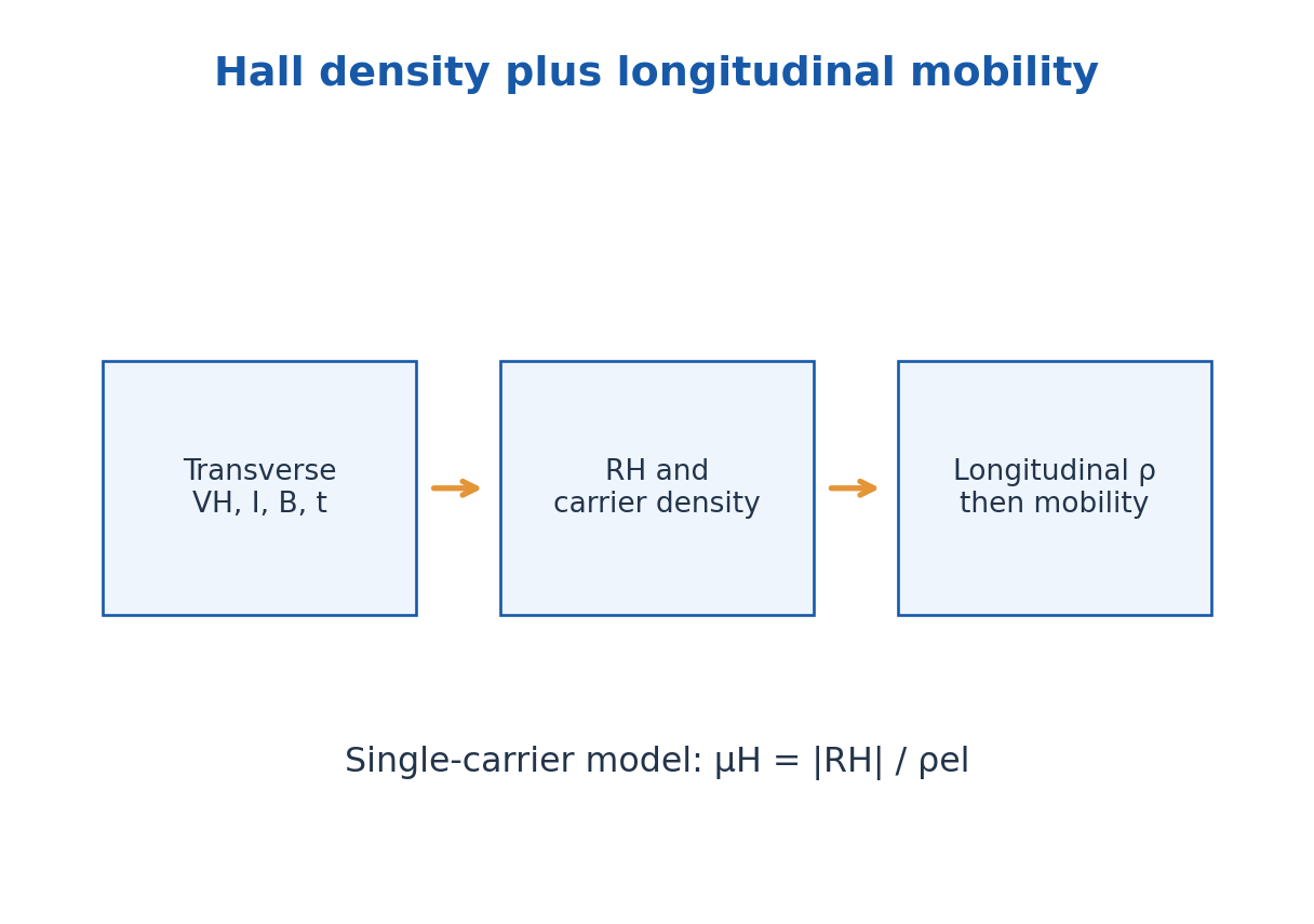
The longitudinal conductivity is σ = neμ for one dominant carrier, giving Hall-mobility magnitude μH = |RH|σ under the simple model. Resistivity is ρel = 1/σ. For a uniform bar, R = ρel L/A; the specimen resistance is not itself a material conductivity.
Concentration in cm^-3 converts to m^-3 by multiplying by 10^6; mobility in cm²/(V s) converts to m²/(V s) by multiplying by 10^-4. The Hall coefficient has units m³/C. Check that RHIB/t produces volts, not a current or field unit.
Experimental offsets from imperfect contact alignment can be reduced by reversing field and current and extracting the component odd in both. Temperature control matters because carrier density and mobility can vary. These procedures support the ideal Hall relation without replacing a proper multicarrier analysis when needed.
Worked Problem 4.34: Hall Mobility from Resistivity
Problem: A one-carrier specimen has |RH| = 5.0 × 10^-4 m³/C and longitudinal resistivity 0.020 ohm m. Find μH.
Method: μH = |RH|σ = |RH|/ρel.
Calculation: σ = 1/0.020 = 50 S/m.
Answer: μH = 0.0250 m²/(V s) = 250 cm²/(V s).
Check: The conductivity is a material value; do not substitute an uncorrected specimen resistance.
Worked Problem 4.35: Removing a Field-Even Hall Offset
Problem: At fixed positive current, voltages at +B and -B are +7.2 mV and -6.8 mV. Extract the field-odd Hall component and field-even offset.
Method: Vodd = [V(+B) – V(-B)]/2; Veven = [V(+B) + V(-B)]/2.
Calculation: Take the half-difference and half-sum.
Answer: Hall component at +B = +7.0 mV; even offset = +0.20 mV.
Check: Further current reversal can reject additional offsets; this two-reading calculation addresses field parity only.
26. E. Thermal Laws and Energy Balance – CE and CH
Temperature describes thermal equilibrium; internal energy is a state function; heat and work are transfers across a system boundary. The zeroth law supports temperature measurement. A thermometer should reach equilibrium without significantly disturbing the sample.
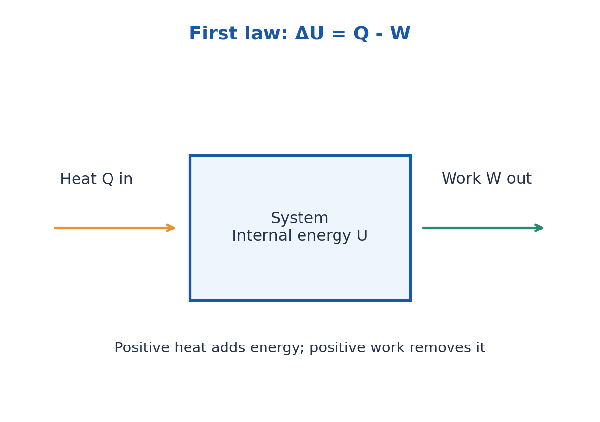
Using work done by the system as positive, the first law is ΔU = Q – W. For a quasistatic expansion W = ∫p dV. Constant-volume heating has no boundary expansion work, whereas an isothermal ideal-gas expansion can absorb heat while maintaining constant internal energy. State the sign convention before calculating.
The second law sets the direction of spontaneous processes and limits heat-engine efficiency. For a reversible transfer dS = δQrev/T; total entropy generation is nonnegative. A heat engine between reservoirs TH and TC cannot exceed Carnot efficiency 1 – TC/TH, with temperatures in kelvin.
The third law concerns the limiting entropy of a perfect crystal as temperature approaches absolute zero. Absolute zero cannot be reached by a finite sequence of ordinary cooling operations.
Engineering thermal processes must satisfy energy conservation and the direction imposed by entropy generation.
Worked Problem 4.36: First Law and Engine Bound
Problem: A closed system receives 1200 J and does 450 J work. Find ΔU. Separately find the reversible maximum engine efficiency between 500 K and 300 K.
Method: ΔU = Q – W; ηmax = 1 – TC/TH.
Calculation: 1200 – 450 = 750; 1 – 300/500 = 0.4.
Answer: ΔU = +750 J; maximum efficiency = 40.0%.
Check: These are separate systems; actual irreversible engine efficiency is lower than its reversible bound.
27. Fourier Conduction and Thermal Conductivity
Conduction transfers energy through microscopic interactions without requiring bulk material flow. In one dimension, qx = -k dT/dx, where qx is flux in W/m² and k is conductivity in W/(m K). The minus sign points the heat flow toward decreasing temperature.
For a uniform slab with constant k, steady one-dimensional conduction and no internal heat generation, Qdot = kA(Th – Tc)/L. A large temperature difference increases heat rate, while a larger thickness reduces it. Thermal conductivity is a material property under stated conditions; conductance kA/L also depends on shape.
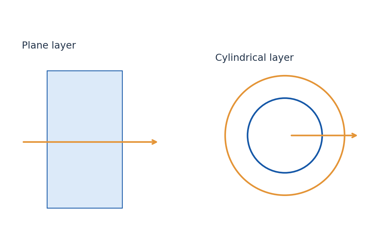
Cylindrical radial conduction has a changing area. For a long hollow cylinder with inner and outer radii r1 and r2, resistance is ln(r2/r1)/(2πkL) under the standard steady assumptions. Do not apply the plane-wall formula using an arbitrary average area without identifying it as an approximation.
Heat capacity controls energy storage, whereas conductivity controls transport for a given gradient. Thermal diffusivity k/(ρc) combines both in a simple transient conduction equation. A steady conductive calculation needs temperatures at the ends of that specific path, not unrelated room or furnace readings.
Worked Problem 4.37: Plane-Wall Heat Rate
Problem: A wall has k = 0.80 W/(m K), area 12 m², thickness 0.20 m and surface difference 15 K. Find steady heat rate.
Method: Qdot = kAΔT/L.
Calculation: Substitute the two actual wall-face temperatures through their difference.
Answer: Qdot = 720 W.
Check: Ambient air temperatures would require film resistances in addition to the wall.
Worked Problem 4.38: Cylindrical Insulation Resistance
Problem: A long cylindrical layer has r1 = 0.020 m, r2 = 0.030 m, k = 0.20 W/(m K) and length 2.0 m. Its radial temperature difference is 30 K. Find resistance and heat rate.
Method: R = ln(r2/r1)/(2πkL).
Calculation: Use the natural logarithm ln1.5.
Answer: R = 0.161329 K/W; heat rate = 185.95490 W.
Check: End effects are neglected. Plane-wall area changes cannot be ignored without a justified approximation.
28. Convection and Thermal Radiation
Convection exchanges energy between a surface and moving fluid. Newton’s boundary relation is Qdot = hA(Ts – Tfluid), with h in W/(m² K). Natural convection is driven by buoyancy associated with density variation; forced convection uses imposed motion such as a fan or pump.
Thermal radiation is electromagnetic transfer and needs no material medium. For a small grey surface exchanging with large isothermal surroundings, net rate is εσSB A(Ts^4 – Tsur^4). Temperatures must be kelvin. Emissivity, geometry and spectral behaviour affect real exchange.
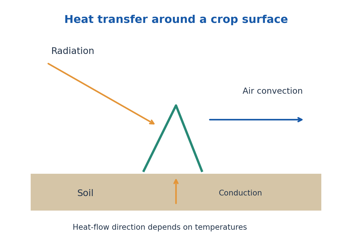
For a stated temperature pair, the simple radiation expression can be written hrA(Ts – Tsur), with hr = εσSB(Ts + Tsur)(Ts² + Tsur²). This effective coefficient generally changes as temperatures change; it is not a universal constant for all cooling intervals.
Convection and radiation can operate in parallel from the same surface, while conduction through a solid often supplies them in series with an interior source. Draw the physical path and label boundary temperatures before combining terms. Adding every available coefficient without a network is not an energy balance.
Worked Problem 4.39: Convection Plus Radiation
Problem: A 1.0 m² surface at 350 K faces large surroundings and air both at 300 K. h = 10 W/(m² K), ε = 0.80. Find net heat rate.
Method: Qdot = hAΔT + εσSB A(Ts^4 – Tsur^4).
Calculation: Convective term = 500 W; calculate radiation using absolute temperatures.
Answer: Radiation = 313.28819 W; total outward heat rate = 813.28819 W.
Check: Both paths share the same surface temperature here, so their rates add in parallel.
29. Heat Capacity, Thermal Conductivity and Expansion
Heat capacity C = dQ/dT under a specified process has units J/K; specific heat c is per unit mass in J/(kg K). For constant-volume and constant-pressure processes the capacities can differ because work differs. For an ideal gas per mole, CP – CV = R. For a finite temperature range use Q = m∫c(T)dT, or mcΔT when c is approximately constant.
Thermal conductivity k controls heat flow under a temperature gradient; heat capacity controls stored energy for a temperature change. They are not interchangeable. A material can conduct heat rapidly while storing comparatively little energy per volume. Diffusivity αth = k/(ρc) combines these effects for a simple medium.
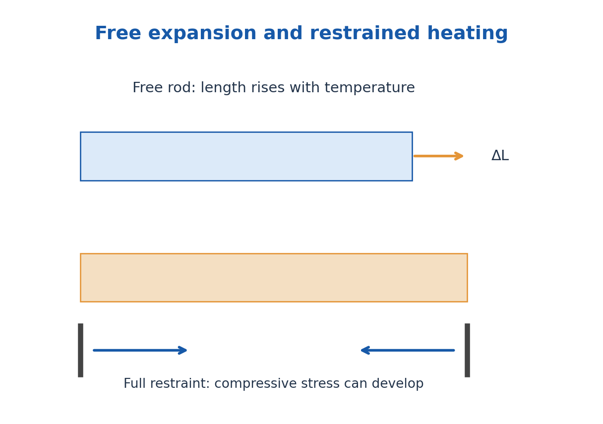
For small temperature changes, linear expansion is ΔL = αL L0ΔT. Isotropic area and volume expansion coefficients are approximately 2αL and 3αL. A hole in a freely expanding plate increases as if the missing material expanded with the plate. Nonuniform temperatures or constraints can produce stress.
Engineering extension: If a uniform linear elastic rod is completely restrained and would otherwise thermally expand, the axial stress magnitude is approximately YαLΔT, provided yielding, buckling and temperature-dependent changes are negligible. Free expansion produces strain without this constraint stress.
Worked Problem 4.40: Expansion of Length and Volume
Problem: An isotropic solid has αL = 10 × 10^-6 K^-1, L0 = 3.0 m and ΔT = 40 K. Find ΔL and approximate fractional volume rise.
Method: ΔL = αL L0ΔT; ΔV/V ≈ 3αLΔT.
Calculation: Linear thermal strain = 4.0 × 10^-4.
Answer: ΔL = 1.20 mm; ΔV/V ≈ 0.00120 = 0.120%.
Check: These are free, small, isotropic expansion estimates.
30. Melting, Solidification and Latent Energy
Heating a single phase generally changes temperature according to Q = m∫c(T)dT, or mcΔT for approximately constant specific heat. During a pure-substance phase change at fixed pressure, energy can change phase fraction without changing the equilibrium transition temperature.
Latent heat of fusion Lf is energy per mass for melting; freezing releases the corresponding latent energy under the same reversible transition conditions. Vaporisation and condensation use Lv. A complete heating calculation adds the sensible and latent terms for each stage in the specified initial-to-final path.
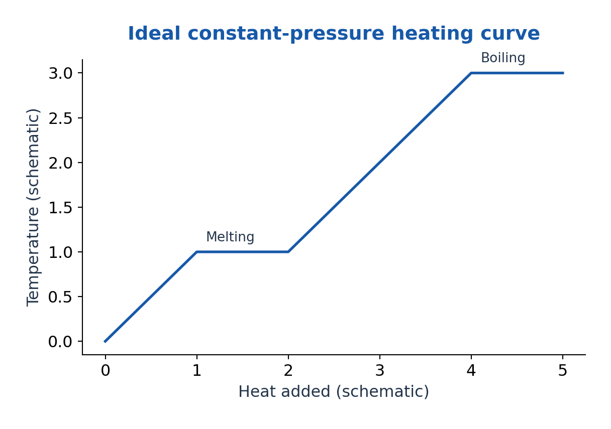
A heating curve for an ideal pure material can show a plateau while solid and liquid coexist. An alloy or impure mixture may transform over a range, and nonuniform heating can obscure an observed plateau. The ideal curve is a model, not a requirement that every measured specimen remain exactly isothermal.
Solidification in construction or process materials releases energy that must be removed. Thermal gradients and expansion or shrinkage can produce stress. A numerical heat total is not a cooling time unless the heat-transfer rate or transient model is also specified.
Worked Problem 4.41: Heat Through Melting and Warming
Problem: Take 0.20 kg ice at 0°C to water at 20°C. Use Lf = 334 kJ/kg and cwater = 4180 J/(kg K). Find heat.
Method: Q = mLf + mcwaterΔT.
Calculation: Latent term = 66800 J; sensible water term = 16720 J.
Answer: Q = 83520 J = 83.52 kJ.
Check: There is no initial ice-warming term because the starting temperature is already the melting point.
31. Enthalpy, Entropy and Equations of State
Enthalpy is H = U + pV. For a constant-pressure closed-system process with only pressure-volume work, heat equals ΔH. In steady flow, enthalpy conveniently incorporates flow work, but kinetic, potential and shaft-work terms may still be required in the full energy equation.
Entropy is a state function. Along a reversible path dS = δQrev/T; for an irreversible process the entropy balance includes generation. For a body with approximately constant specific heat heated reversibly from T1 to T2, ΔS = mc ln(T2/T1). Use absolute temperatures in the ratio.
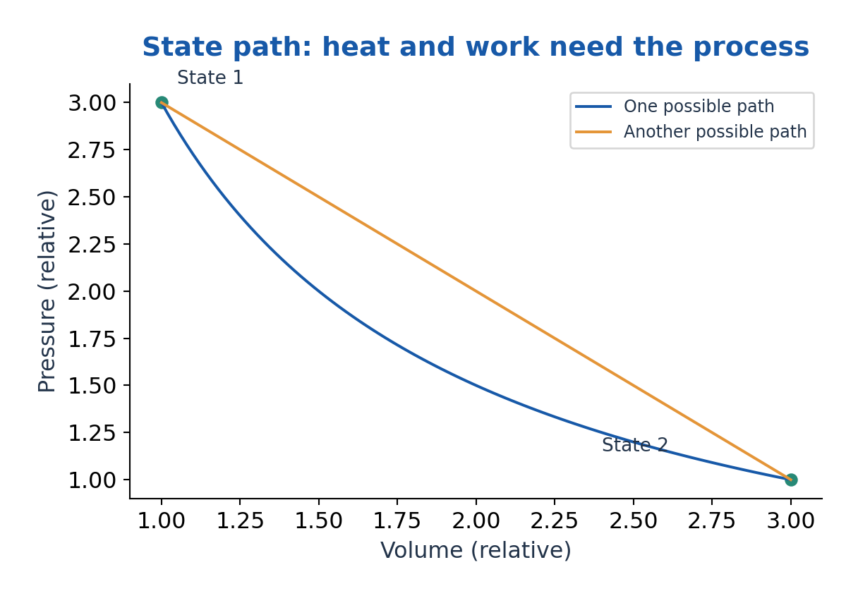
For a reversible isothermal phase change, ΔS = mL/T. A system’s entropy may decrease when it exports heat, while total entropy of system plus surroundings cannot decrease for an isolated overall process. Heat transfer and entropy are therefore not interchangeable quantities.
An ideal gas equation of state is pV = nRT. For n moles, ΔU = nCVΔT when molar CV is constant. Real gases can deviate, particularly near transitions or at high density; a van der Waals model uses (p + a/Vm²)(Vm – b) = RT per mole to represent attractions and finite volume approximately.
Worked Problem 4.42: Entropy Change and Ideal Gas Pressure
Problem: A 1.0 kg body with c = 500 J/(kg K) is heated reversibly from 300 to 330 K. Find ΔS. Separately find p for 2.0 mol ideal gas at 300 K in 0.050 m³.
Method: ΔS = mc ln(T2/T1); p = nRT/V.
Calculation: Use ln(330/300) and absolute gas temperature.
Answer: ΔS = 47.65509 J/K; gas pressure = 99.77355 kPa.
Check: The entropy result assumes constant specific heat over the interval; the gas result assumes ideal behaviour.
32. Thermal Resistance Networks and Boundary Temperatures
For a uniform plane slab, resistance is L/(kA); for a convective film it is 1/(hA). Resistances in a single steady series path add, giving Qdot = ΔT/Rtotal. The same heat rate passes through each element while each carries its own temperature drop.
For two independent paths between the same temperature nodes, conductances add: 1/Req = 1/R1 + 1/R2. A composite wall can have both series layers and parallel regions. Contact resistance and thermal bridges can alter practical performance even when individual material conductivities are known.
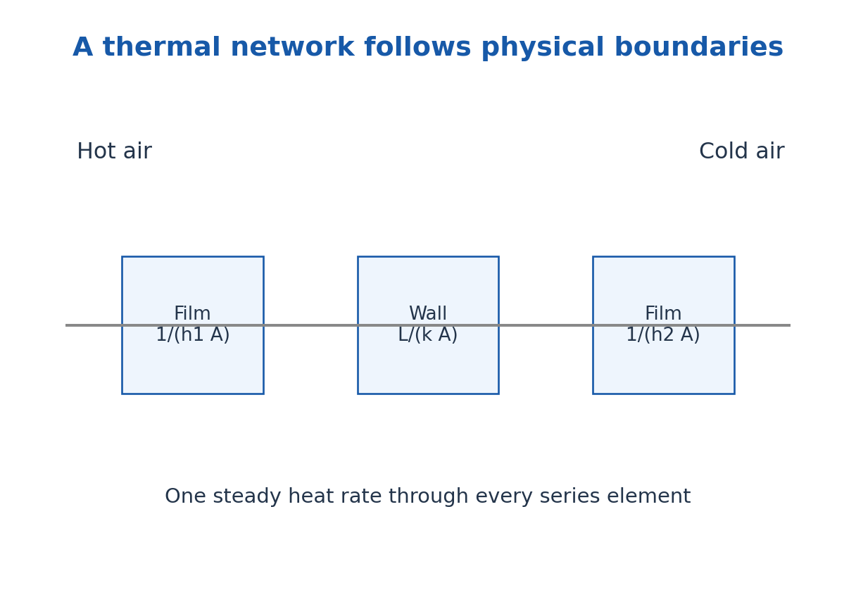
For a cylindrical layer use the appropriate logarithmic resistance, and use the actual surface area for each convective film. Inner and outer cylinder areas differ. A single film coefficient should not be multiplied by an unrelated cross-sectional area.
Start at a named hot node, trace every energy path to a named cold node, and check whether accumulation can be neglected. If the body is heating or cooling, include thermal storage; a steady network alone cannot determine its entire time evolution.
Worked Problem 4.43: Series Thermal Network
Problem: A 0.10 m wall with k = 0.50 W/(m K), area 2.0 m², has films h1 = 20 and h2 = 10 W/(m² K). Ambient difference is 30 K. Find heat rate.
Method: Rtotal = 1/(h1A) + L/(kA) + 1/(h2A).
Calculation: Rtotal = 0.025 + 0.100 + 0.050 = 0.175 K/W.
Answer: Heat rate = 171.42857 W.
Check: All three elements carry one steady rate. The ambient difference spans the full network.
33. Newton Cooling Law and Lumped Transient Response
In one-dimensional steady conduction through a uniform slab, thermal resistance is Rth = L/(kA) and heat rate is ΔT/Rth. Resistances in series add. A convective film has resistance 1/(hA). Contact resistance or radiation can add other paths; the correct network follows the actual physical boundaries.
Newton’s cooling law in lumped form gives mc dT/dt = -hA(T – T∞) when h, area, heat capacity and surroundings are constant and internal temperature gradients are negligible. The solution is T – T∞ = (T0 – T∞)exp(-t/τth), with τth = mc/(hA).
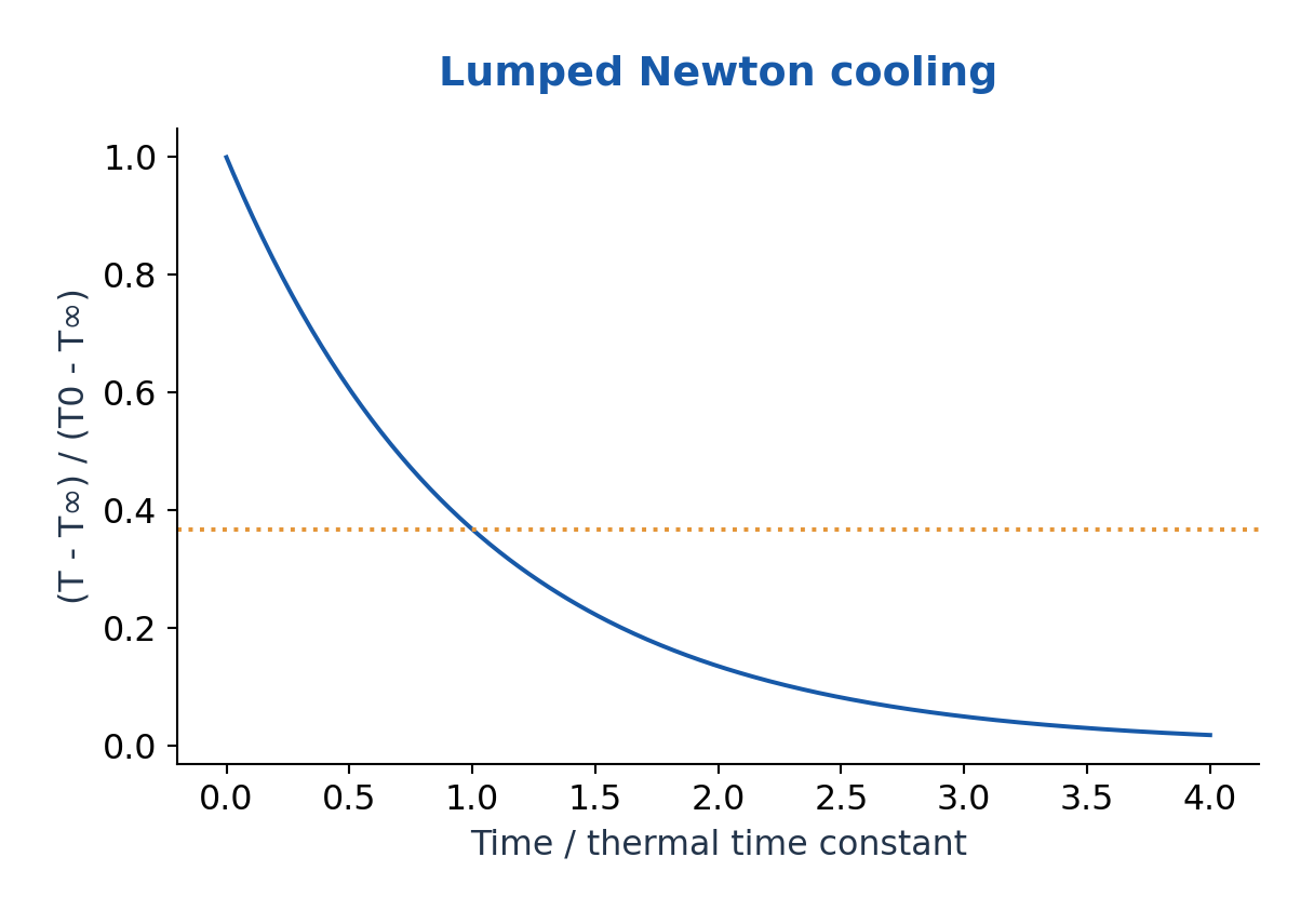
The lumped approximation is commonly checked by Bi = hLc/k much less than one, often using Bi < 0.1 as a practical criterion with characteristic length Lc = V/A. This concerns internal uniformity; it is not a statement that cooling is always slow.
For radiative cooling over a large temperature range, heat rate is not simply proportional to Celsius temperature difference; use the fourth-power law or a justified local linearisation. A measured cooling curve can estimate a model parameter, but heat leaks, evaporation and changing airflow may invalidate a single exponential fit.
Worked Problem 4.44: Cooling Time and Lumped Validity
Problem: A body has τth = 400 s and cools from 90°C toward 30°C. Find time to 50°C. Given h = 10 W/(m² K), Lc = 0.005 m and k = 5 W/(m K), evaluate Bi.
Method: t = τth ln[(T0 – T∞)/(T – T∞)]; Bi = hLc/k.
Calculation: Difference ratio = 60/20 = 3; Bi = 10 × 0.005/5.
Answer: t = 439.44492 s; Bi = 0.010, supporting the lumped approximation.
Check: A small Bi helps internal uniformity; it does not prove every boundary coefficient is constant.
34. F. Solar Radiation and the Agricultural Surface – AG
Solar radiation supplies the main external energy source for crop and soil systems. Direct radiation arrives from the solar direction, diffuse radiation is scattered by the atmosphere and clouds, and reflected radiation comes from surrounding surfaces. Global horizontal radiation is the combined direct contribution on that plane and diffuse component.
Shortwave radiation is partly reflected according to surface albedo, partly transmitted through a canopy and partly absorbed. Absorbed energy can support photosynthesis but much is redistributed as sensible heat, latent heat and storage. Incoming solar energy is not identical to useful biochemical energy.
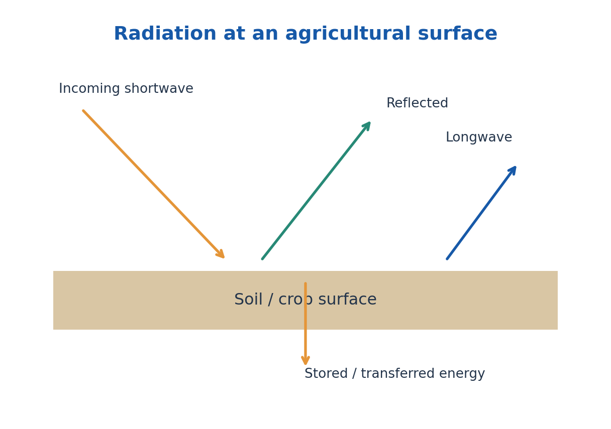
Photosynthetically active radiation is conventionally the 400–700 nm band. Photon-flux and energy-flux measures are different; conversion requires spectral information or a stated representative wavelength. A light reading should specify the spectral response and units.
Net radiation includes the shortwave balance and longwave exchange with atmosphere and surroundings. A simple surface balance is Rn = H + LE + G when storage and other terms are negligible, using upward sensible and latent flux and downward ground flux as positive losses. Declare the convention before solving.
Worked Problem 4.45: Absorbed Shortwave Energy
Problem: A surface receives 600 W/m² and has albedo 0.20, with no shortwave transmission. Find reflected and absorbed shortwave flux, and absorbed energy over 5.0 h at this constant rate.
Method: Reflected = albedo × incoming; absorbed = remainder.
Calculation: Reflected = 120 W/m²; absorbed = 480 W/m²; duration = 18000 s.
Answer: Absorbed shortwave = 480 W/m²; energy = 8.64 MJ/m².
Check: This is not full net radiation; longwave exchange and non-radiative fluxes are separate.
35. Crop-Radiation Interaction and Canopy Effects
Leaves reflect, transmit and absorb different wavelength bands differently. Chlorophyll absorption supports photosynthetic processes, while canopy structure and near-infrared scattering affect energy distribution. Leaf angle, density, row geometry and sun position influence the light reaching lower leaves and soil.
A simple attenuation model is I = I0 exp(-kext LAI), where LAI is leaf area per ground area and kext is an effective extinction coefficient under the stated geometry. The intercepted fraction is 1 – I/I0. Real canopies require treatment of direct/diffuse light, clumping and spectral differences for detailed prediction.
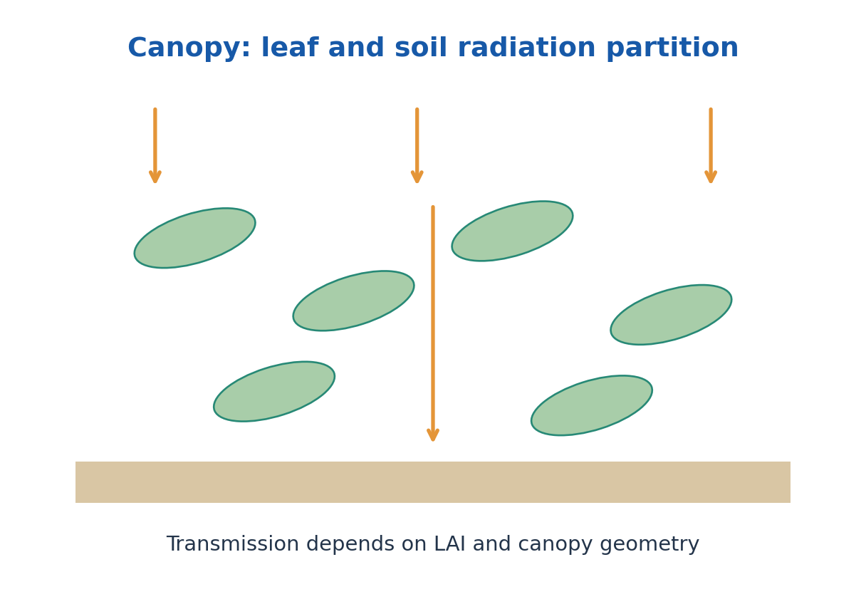
Crop response is not indefinitely proportional to incident radiation: light saturation, temperature, carbon supply and water status can limit growth. Shading can reduce radiation stress but may also reduce photosynthetic input. Its value depends on crop and environment rather than on one universal percentage.
A canopy changes the soil surface through shade, wind reduction, humidity and interception of rain. Mulch and row cover further alter reflection, evaporation and heat exchange. A good explanation connects the optical change with the resulting water and energy balance instead of equating every cooler surface with improved crop performance.
Worked Problem 4.46: Canopy Transmission
Problem: Use I/I0 = exp(-kext LAI) with kext = 0.60 and LAI = 3.0. Find transmitted and intercepted fractions.
Method: Evaluate exp(-1.8), then subtract from one.
Calculation: The extinction coefficient is an effective supplied canopy value.
Answer: Transmitted = 0.16530; intercepted = 0.83470.
Check: Interception alone does not give photosynthetic efficiency or yield.
36. Microclimate and Crop-Scale Energy Exchange
Microclimate is the local atmospheric and surface environment over a small region such as within a canopy or near a soil surface. It can differ from a standard weather-station reading because shading, transpiration, wind shelter, surface colour and moisture change the local energy exchanges.
Leaf temperature follows an energy balance involving absorbed radiation, thermal emission, convection, latent transfer and short-term storage. Transpiration can cool a leaf when water is available and stomatal conditions permit it. A leaf can also be warmer or cooler than the air, so air temperature alone does not specify every plant temperature.
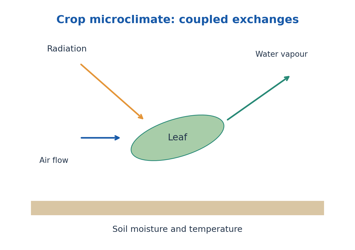
Wind generally changes convective and vapour transfer; humidity changes the vapour-pressure driving force. Shelter can reduce damaging wind but may also alter cooling and moisture persistence. Irrigation changes evaporation and thermal storage, not merely the amount of soil water.
Protected cultivation controls microclimate through ventilation, shading, heating, evaporative cooling and moisture management. Measure representative positions and times. A single sensor immediately beside a heater or wet patch can misrepresent the crop zone.
37. Weather Parameters, Humidity and Instruments
Weather describes atmospheric conditions over relatively short intervals; climate describes statistical behaviour over longer periods and includes variability and extremes. Important agricultural parameters include air temperature, humidity, wind, rainfall, radiation and sometimes pressure and soil temperature.
Relative humidity is RH = 100 ea/es(T), where ea is actual vapour pressure and es is saturation vapour pressure at the stated temperature. Vapour-pressure deficit is VPD = es – ea. Heating air without adding moisture can lower RH because saturation pressure rises; the moisture amount and percentage saturation are different ideas.
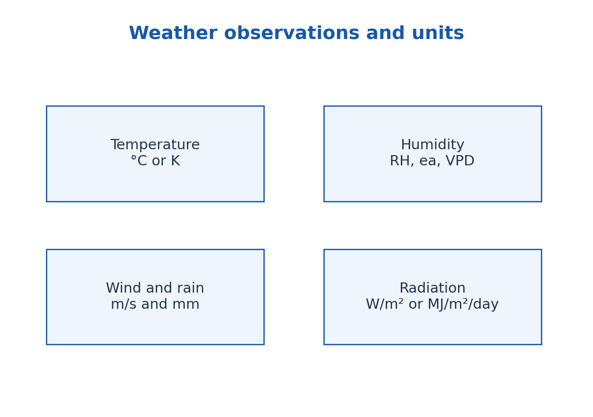
Thermometers or electronic sensors measure temperature, hygrometers humidity, anemometers wind speed, rain gauges precipitation depth and pyranometers broad shortwave radiation under their calibration. A soil probe measures at its actual burial depth. Shelter, radiation shielding and siting are essential to interpreting a reading.
Wind height, sensor exposure, time averaging and units should accompany comparisons. Rainfall in millimetres is a water-volume-per-area measure, not a flow rate by itself. Radiation in W/m² is instantaneous or averaged power per area, while MJ/m²/day expresses accumulated daily energy.
Worked Problem 4.47: Humidity and Vapour-Pressure Deficit
Problem: At the stated temperature, saturation vapour pressure is 3.2 kPa and actual vapour pressure is 2.0 kPa. Find RH and VPD.
Method: RH = 100 ea/es; VPD = es – ea.
Calculation: RH = 100 × 2.0/3.2.
Answer: RH = 62.5%; VPD = 1.2 kPa.
Check: Relative humidity and actual vapour pressure are different descriptors; temperature changes the saturation value.
Worked Problem 4.48: Rainfall Depth to Water Volume
Problem: A 12 mm rainfall event falls uniformly over 2.0 hectares. Estimate the gross water volume before runoff or other losses.
Method: V = depth × area.
Calculation: 12 mm = 0.012 m; 2.0 ha = 20000 m².
Answer: Gross volume = 240 m³.
Check: This is not the infiltrated or crop-available amount unless losses and storage are assessed.
38. Greenhouse Effect, Climate Change and Agricultural Impacts
The atmospheric greenhouse effect arises because greenhouse gases absorb and emit terrestrial infrared radiation, changing the radiative exchange between surface, atmosphere and space. It is not caused by an ozone hole admitting all extra solar heat. The natural effect contributes to surface warmth; increasing greenhouse-gas concentrations alters the planetary energy balance.
A glasshouse also warms through changes in convection and ventilation, as well as radiation. Therefore a physical greenhouse enclosure and the atmospheric greenhouse effect are not identical mechanisms. Use an energy-flow diagram rather than saying that all heat is permanently trapped.
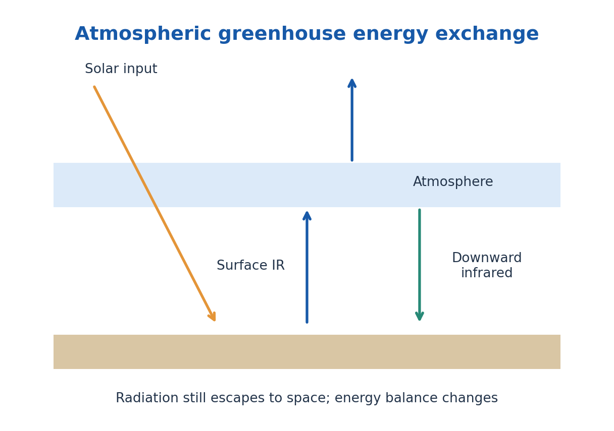
Climate change involves persistent shifts in climate statistics, including mean conditions and some extremes. One unusually hot or cold day alone does not establish or refute a long-term trend. Agricultural effects can involve heat stress, water demand, altered seasonality, pests and extreme-event risk, with differences across crops and regions.
Mitigation reduces the drivers, for example through lower emissions or changes in energy use.
Adaptation reduces harm under changing conditions, for example altered sowing dates, water management and crop choices. Evaluate a proposed response using its local water, energy, cost and environmental implications.
39. Air Pollution: Transport, Exposure and Crop Response
Air pollutants include particulate matter and gases such as ozone, nitrogen oxides and sulfur dioxide. Sources, chemical formation, transport, deposition and exposure determine effects. Ground-level ozone is a pollutant formed through atmospheric reactions; stratospheric ozone has a different protective role.
Wind transports pollutants, atmospheric turbulence disperses them and deposition transfers them to surfaces. A temperature inversion can suppress vertical mixing, increasing near-surface concentrations under suitable conditions. The emission rate alone does not determine the concentration at a crop or settlement.
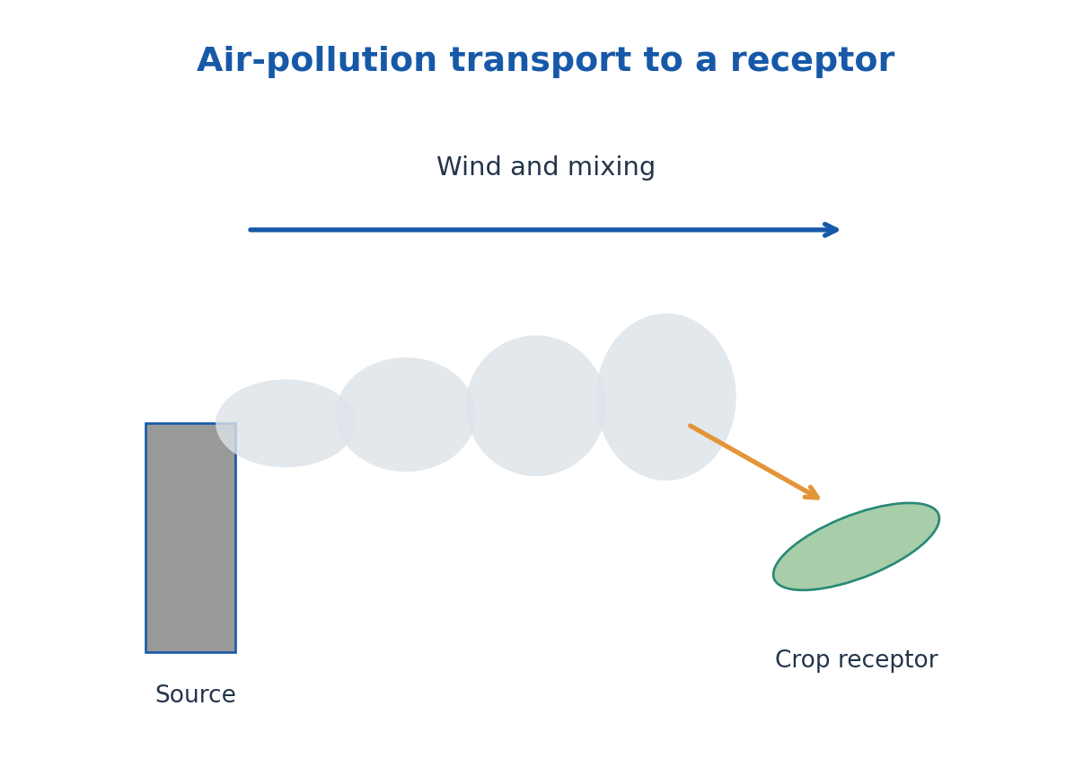
Particles can reduce light and deposit on leaves, while some gases enter through stomata and affect plant processes. Effects depend on concentration, duration, species, moisture and environmental context. A mass concentration such as micrograms per cubic metre is not the same as total emitted mass or dose.
Control can reduce emissions at source, capture particles or gases, change fuel or process conditions and monitor exposure. Vegetation can affect local deposition and flow but is not a complete substitute for source control. Use physical transport and measurement concepts when comparing interventions.
Worked Problem 4.49: Pollutant Mass in an Air Volume
Problem: Air concentration is 80 microg/m³ in a well-mixed 5000 m³ ideal control volume. Find contained pollutant mass.
Method: Mass = concentration × volume.
Calculation: 80 × 5000 = 400000 microg.
Answer: Mass = 0.400 g.
Check: This is instantaneous contained mass under the mixing assumption, not an emission rate or personal exposure dose.
40. Water Pollution: Physical Indicators and Conservation
Water pollution changes water quality through physical, chemical or biological contamination. Physical indicators include turbidity, temperature, colour and suspended solids. A clear appearance does not prove safe water, and high turbidity is not a direct numerical measure of every dissolved contaminant.
Dissolved oxygen supports aquatic processes and depends on temperature, mixing and biological demand. Oxygen-demand measurements and dissolved concentration represent different quantities. Thermal pollution can alter oxygen availability and organism conditions even when no visible solid waste is added.
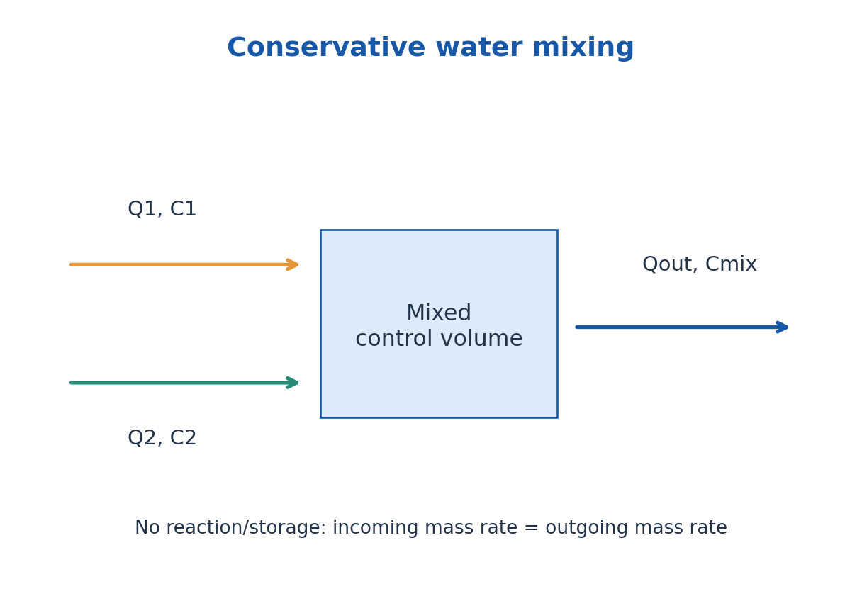
For a fully mixed conservative solute without reaction or loss, incoming mass rates add: Cmix = (Q1C1 + Q2C2)/(Q1 + Q2). This is a model with explicitly conserved substance. Settling, chemical transformation, volatilisation or biological uptake require additional terms.
Sedimentation removes some settleable particles; filtration separates according to filter and particle properties; aeration enhances gas exchange; biological and chemical treatment address other contaminants. Dilution lowers concentration under its assumptions but does not remove the pollutant mass. Agricultural management must consider both concentration and total loading.
Worked Problem 4.50: Conservative Water Mixing
Problem: A stream of 0.020 m³/s at 10 mg/L mixes completely with 0.005 m³/s at 50 mg/L. Find mixed concentration and outgoing pollutant load.
Method: Cmix = (Q1C1 + Q2C2)/(Q1 + Q2); convert concentration to kg/m³ for load.
Calculation: Cmix = (0.020 × 10 + 0.005 × 50)/0.025 = 18 mg/L; 18 mg/L = 0.018 kg/m³.
Answer: Mixed concentration = 18 mg/L; load = 0.000450 kg/s = 0.450 g/s.
Check: Mixing reduces or raises concentration according to the flows but conserves total pollutant mass for this model.
Complete Derivations and Exam Explanations
1. Fibre Acceptance: Connect the Two Refractions
Let θ1 be the meridional ray angle to the fibre axis inside the core and θa its maximum external entrance angle. At the core-cladding wall, incidence to the normal is 90° – θ1. At the limiting guided case that angle equals ic, where sin ic = n2/n1.
Therefore sinθ1,max = cos ic = √[1 – (n2/n1)²]. The entrance face is perpendicular to the axis, so Snell’s law gives n0 sinθa = n1 sinθ1,max. Substitute the preceding relation to obtain NA = n0 sinθa = √(n1² – n2²). The external and internal angles arise at different interfaces and use different reference lines.
For Δ = (n1 – n2)/n1, write n2 = n1(1 – Δ). Then NA² = n1²[1 – (1 – Δ)²] = n1²(2Δ – Δ²). Neglecting Δ² only when Δ is small yields NA ≈ n1√(2Δ). The exact formula is available when this approximation is not satisfactory.
The full acceptance cone is twice the half-angle. In a medium with n0 greater than one, the same NA corresponds to a smaller θa. The derivation assumes the ideal step-index meridional-ray geometry; it does not establish a complete optical-power coupling efficiency or a mode spectrum.
2. Einstein Balance and Why Pumping Is Necessary
For two levels at thermal equilibrium, upward absorption balances downward spontaneous plus stimulated emission: N1B12uν = N2A21 + N2B21uν. Rearrangement gives uν = A21/[(N1/N2)B12 – B21]. The population ratio includes level degeneracies and the Boltzmann energy factor.
Substitute N1/N2 = (g1/g2)exp(hν/kBT). Comparing the expression with Planck’s spectral radiation law for frequency in vacuum identifies g1B12 = g2B21 and A21/B21 = 8πhν³/c³. If the radiation convention uses angular frequency or a different density definition, the displayed coefficient relation must be adjusted consistently.
The competing stimulated contributions are N2B21uν and N1B12uν. Net stimulated gain requires N2/g2 > N1/g1. Equilibrium at positive temperature does not maintain that condition. A pump and suitable relaxation pathways move the system out of equilibrium.
This explains the use of metastable upper levels and rapidly emptied lower levels. In ruby, the lower laser manifold is the ground manifold and substantial pumping is required. In a common He-Ne system, discharge excitation and helium-to-neon energy transfer help maintain the relevant neon population distribution. Merely putting two mirrors around a thermal lamp does not create this inversion.
3. Laser Round-Trip Threshold and the Output Trade-Off
Follow one intensity component for one complete round trip. It crosses the active length L twice and therefore receives net distributed factor exp[2(g – α)L], with g the small-signal intensity gain and α the intensity loss per length. Reflection at the mirrors multiplies it by R1R2.
At threshold the round-trip multiplier equals one: R1R2 exp[2(g – α)L] = 1. Taking natural logarithms and isolating g gives gth = α + ln[1/(R1R2)]/(2L). Distributed and mirror losses thus enter the same threshold balance, but through different terms.
A more transmitting output coupler can extract more light on a pass but also lowers its reflectivity and raises the required gain, all else equal. It is therefore not valid to predict output by maximising transmission alone. Above threshold, gain saturation and pump balance determine the steady result.
This calculation uses intensity reflectivities and coefficients. A field-amplitude propagation model uses square roots or different factors and cannot be mixed into the same formula without conversion. Explain the convention in a numerical answer before assigning a threshold value.
4. Ultrasonic Generators, Reception and Depth Measurement
A magnetostrictive system converts an electrically produced magnetic variation into rod strain. A piezoelectric generator converts an electric field directly into elastic strain through the converse effect. Both require a mechanical mode and coupling into the intended acoustic medium, but their transduction mechanisms are different.
For a simple free-free longitudinal rod, a half-wavelength fits the length in the fundamental mode, giving λ = 2L and f = v/(2L). With ideal slender-rod v ≈ √(Y/ρ), this gives the quoted resonance estimate. A simple plate thickness mode similarly uses λ ≈ 2t, but the relevant elastic constant and electrical boundary conditions determine its mode speed.
A returning echo applies stress to a piezoelectric receiver and produces charge through the direct effect. If the same element sends and receives, the electronic chain must distinguish the outgoing pulse and later weak return. A sound couplant reduces an unwanted air interface; the acoustic impedance mismatch controls reflected and transmitted fractions under the appropriate boundary model.
For a straight pulse-echo path to a reflector at depth d, total distance is 2d. With known speed v and round-trip delay Δt, 2d = vΔt and d = vΔt/2. A through-transmission timing setup measures a different path. Attenuation, coupling and reflection all affect echo amplitude, so amplitude alone does not uniquely specify depth or flaw size.
5. Dielectric Energy and Magnetic-Loop Interpretation
For an ideal capacitor, U = Q²/(2C) = CV²/2. Inserting a dielectric increases capacitance under the same geometry. If it remains connected to a fixed-voltage source, U rises and extra charge enters. If it is disconnected with fixed charge, U falls. The difference follows from the electrical boundary condition, not a contradiction in energy conservation.
A real dielectric can have polarisation lag, conduction and breakdown limits. Under a stated small-loss sinusoidal model, power loss is ωC Vrms² tanδ. The frequency, capacitance, voltage convention and definition of the loss term all matter. A high storage response alone does not determine safe operating field or low dissipation.
For a ferromagnetic B-H cycle, remanence is the remaining B at H = 0 on the specified history branch; coercivity is the reverse H needed to reach B = 0. Loop area is dissipated energy per volume per cycle. Multiplying by actual volume gives specimen energy; multiplying again by frequency estimates its hysteresis power if the loop remains unchanged.
A narrow suitable loop benefits repeated reversal, while high coercivity and retention benefit permanent magnets. Add eddy-current and other losses separately when modelling an AC core. The loop’s nonlinear history dependence is not described by applying one constant susceptibility over every field.
6. Hall Coefficient and One-Carrier Density: Keep the Signs Explicit
Choose current along +x and magnetic field along +z. Define RH = Ey/(JxBz). A carrier with signed charge q and drift velocity v satisfies zero transverse net force at the ideal steady balance: Ey + (v × B)y = 0. With velocity along x, the cross-product y component is -vxBz, so Ey = vxBz.
Current density is Jx = nqvx. Dividing the balancing electric field by JxBz therefore gives RH = 1/(nq). This is negative for electrons and positive for holes within the one-carrier isotropic model. The sign statement must accompany the chosen directions and measured contact polarity.
A slab of width w and thickness t has Jx = I/(wt). Define VH = Eyw, equivalent to potential at lower y minus that at upper y. Substitution gives VH = RH IBz/t, so RH = VHt/(IBz). Density magnitude is 1/(e|RH|). Longitudinal conductivity then gives μH = |RH|σ under the same simple assumptions.
Contact misalignment can introduce a voltage even in magnetic field. The half-difference between +B and -B readings isolates the odd contribution at fixed current. Combining field and current reversal improves rejection of further offsets. None of these corrections makes a multicarrier specimen obey the one-carrier density formula; that physical assumption remains to be checked.
7. Thermal Network, Entropy and Cooling as Different Questions
A steady resistance network asks for heat rate under fixed endpoint temperatures. For a plane layer, integrating Fourier’s law with constant area gives resistance L/(kA). For a cylinder the conducting area is 2πrL and integration gives ln(r2/r1)/(2πkL). Convective films use their own surface areas and resistances 1/(hA).
The same heat rate crosses a series path, while parallel paths share temperature nodes and their rates add. Once the heat rate is known, each element’s temperature drop follows Qdot R. This is more informative than assuming ambient and surface temperatures are interchangeable.
An entropy question instead concerns a state change or generation. For a reversible constant-specific-heat path, ΔS = ∫mc dT/T = mc ln(T2/T1). For a reversible isothermal phase transition, ΔS = mL/T. A real irreversible path can have extra entropy generation even when its state-function change is computed using a convenient reversible path.
A cooling-time question requires storage. With a uniform body temperature, constant h and surroundings, mc dT/dt = -hA(T – T∞). Integrate to the exponential difference law. The lumped assumption can be supported by a small Biot number, but radiation, evaporation or changing boundary flow can still invalidate a single constant-coefficient fit.
8. AG: Connect Radiation, Microclimate and Pollution Balances
Incoming shortwave energy is divided into reflected, transmitted and absorbed parts. If transmission is negligible, absorbed shortwave equals (1 – albedo) times incoming radiation. This is not yet net radiation because longwave exchange also contributes. A canopy modifies both the shortwave partition and the wind and vapour environment near leaves and soil.
At the crop surface, a stated balance can distribute net radiation into sensible heating, latent energy, ground heat and storage. Weather parameters influence these paths differently. Wind changes transfer, actual vapour pressure and saturation pressure determine vapour deficit, and water availability constrains evaporation. One local air-temperature reading therefore does not specify the whole crop microclimate.
The same conservation approach helps interpret pollution. In a complete steady conservative water mixing problem, sum incoming mass rates QiCi and divide by outgoing volume rate to obtain concentration. Mixing changes concentration but does not destroy mass. A reactive or settling pollutant needs explicit removal, reaction or storage terms.
Air concentration likewise depends on emission, transport, mixing and deposition, rather than only on source mass. Temperature inversions can inhibit vertical mixing and raise near-surface accumulation under suitable conditions. Correct units separate concentration, stored mass, flux, emission rate and exposure. A credible agricultural explanation connects the measured quantity to its control volume and transport path.
9. CE/CH: Derive Cylindrical Thermal Resistance
Take a long hollow cylinder with constant conductivity k and steady purely radial heat flow. At radius r the conducting area is 2πrL. Fourier’s law gives Qdot = -2πkLr dT/dr. With no internal generation or axial loss, Qdot is independent of radius.
Separate variables: dT = -[Qdot/(2πkL)]dr/r. Integrate from inner radius r1 at T1 to outer radius r2 at T2. Then T2 – T1 = -[Qdot/(2πkL)]ln(r2/r1). Therefore Qdot = 2πkL(T1 – T2)/ln(r2/r1), and the corresponding resistance is ln(r2/r1)/(2πkL).
If r2 > r1 and T1 > T2, the heat rate is positive outward. Add inner and outer film resistances using their own areas 2πr1L and 2πr2L when ambient temperatures are the endpoint nodes. End effects, variable conductivity or heat generation need a more general balance.
10. AG: Move Correctly Between Flux, Total and Concentration
A radiation flux in W/m² is energy per time per area. To find accumulated energy under a constant flux, multiply by duration; multiply by area as well to obtain a whole-field total. For changing radiation, integrate over time rather than multiplying one unrepresentative peak reading by an entire day.
Rainfall depth is already volume per ground area. Converting millimetres to metres and multiplying by the catchment area gives gross water volume, not necessarily infiltration. Runoff, interception, evaporation and storage determine how the water is partitioned.
Pollutant concentration becomes a mass when multiplied by the corresponding water or air volume. It becomes a transported mass rate when multiplied by volume flow rate. For example, one mg/L equals one g/m³ or 0.001 kg/m³. This conversion makes the steady mixing equation a mass-conservation calculation rather than an arithmetic average of concentrations.
Formulas and Model Conditions
| Topic | Relation / Condition |
|---|---|
| Fibre guidance | ic = sin^-1(n2/n1), angle to internal interface normal; n1 > n2 |
| Acceptance | NA = n0 sinθa = √(n1² – n2²); full cone = 2θa |
| Small index step | Δ = (n1 – n2)/n1; NA ≈ n1√(2Δ) only for small Δ |
| Power loss | P = P0 exp(-αpL); loss(dB) = 10 log10(Pin/Pout) |
| Photon | Eph = hν = hc/λ; rate = optical power/Eph |
| Einstein | g1B12 = g2B21; A21/B21 = 8πhν³/c³: vacuum spectral-frequency convention |
| Laser threshold | gth = α + ln[1/(R1R2)]/(2L): intensity gain/loss and reflectivities |
| Ultrasound | v = fλ; Z = ρv; ideal reflected intensity fraction = [(Z2 – Z1)/(Z2 + Z1)]² |
| Resonance | Rod f ≈ √(Y/ρ)/(2L); plate f ≈ v/(2t): stated ideal mode and boundaries |
| Echo | Depth = vΔt/2 for a round trip; one-way transmission uses its actual path |
| Dielectric | D = ε0E + P; P = ε0χeE; εr = 1 + χe in a linear isotropic model |
| Capacitor loss | Ploss ≈ ωC Vrms² tanδ for the stated equivalent small-loss model |
| Magnetic | B = μ0(H + M); weak linear M = χmH; loop area = loss energy/volume/cycle |
| ME piezoelectric | Q = dF and ideal open-circuit V = Q/C in a stated 1D sensor model |
| ME Hall | RH = Ey/(JxBz); VH = Eyw = RHIBz/t; RH = 1/(nq) for one carrier |
| ME mobility | μH = |RH|σ = |RH|/ρel under the one-carrier model |
| First law | ΔU = Q – W: positive W done by the system |
| Thermal paths | Rslab = L/(kA); Rfilm = 1/(hA); Rcyl = ln(r2/r1)/(2πkL) |
| Radiation | Qdot = εσSB A(Ts^4 – Tsur^4): kelvin and stated geometry |
| Thermal storage | Q = mcΔT within one phase; Qlatent = mL at the stated transition |
| Entropy / state | H = U + pV; ΔS = mc ln(T2/T1) for constant c; ideal pV = nRT |
| Cooling | T – T∞ = (T0 – T∞)exp(-t/τth); τth = mc/(hA), lumped model |
| AG radiation | Absorbed shortwave = (1 – albedo) incoming when transmission is zero |
| AG canopy | I/I0 = exp(-kext LAI): supplied effective canopy model |
| AG humidity | RH = 100ea/es(T); VPD = es(T) – ea |
| AG mixing | Cmix = sum(QiCi)/sum(Qi): steady complete conservative mixing |
Conversions:
- 1 nm = 10^-9 m.
- 1 micrometre = 10^-6 m.
- 1 cm^-3 = 10^6 m^-3.
- 1 cm²/(V s) = 10^-4 m²/(V s).
- 1 mg/L = 0.001 kg/m³.
- 1 hectare = 10000 m².
Keep intensity and amplitude attenuation conventions separate.
Constants and Final Check
c = 2.99792458 × 10^8 m/s.
h = 6.62607015 × 10^-34 J s.
e = 1.602176634 × 10^-19 C.
ε0 ≈ 8.8541878 × 10^-12 F/m.
μ0 ≈ 1.2566371 × 10^-6 H/m.
σSB ≈ 5.6703744 × 10^-8 W/(m² K^4).
Physical checks: Check angle and voltage references, wave and loss conventions, thermal endpoint temperatures and pollutant mass conservation before accepting an answer.
Answered Revision Checks
What Must Be True for Total Internal Reflection?
The wave must approach the lower-index medium from the higher-index side, with internal incidence greater than the critical angle measured from the normal.
Why Does External Medium Index Enter Acceptance?
The entrance face refracts light before it reaches the core-cladding interface. Snell’s law introduces n0 into n0 sinθa.
Are Attenuation and Dispersion the Same Limit?
No. One lowers optical power while the other spreads pulse arrival times. Either can limit a link independently.
Can Einstein A/B Be a Dimensionless Rate Ratio?
No. Under the stated convention it has spectral-energy-density units. The rate ratio includes the actual radiation density.
Which Species Gives the Red He-Ne Output?
Neon emits the 632.8 nm laser line. Helium transfers excitation energy through collisions.
Why Can Magnetostrictive Frequency Double?
When unbiased strain is approximately proportional to H², a sinusoidal field contains a strain component at twice the drive frequency.
Does Pulse-Echo Depth Equal vΔt?
That product is the round-trip distance. Divide by two for the reflector depth in the simple straight-path model.
Does a Higher Dielectric Constant Imply Higher Breakdown Strength?
No. Polarisation response, loss, leakage and breakdown are separate properties affected by structure and conditions.
Why Are Hard and Soft Magnetic Materials Different Choices?
They serve different retention and reversal requirements; mechanical hardness is not the definition of the magnetic labels.
When Does Hall Coefficient Equal Inverse Signed Density?
In the stated single-carrier isotropic model. Multicarrier response, mobility weighting and material details can invalidate that simple inference.
Does Dielectric Insertion Always Increase Capacitor Energy?
No. At fixed voltage it increases stored energy, while at fixed isolated charge increasing capacitance lowers stored energy.
Why Does Cylindrical Thermal Resistance Contain a Logarithm?
The conducting area changes with radius, so integrating the radial temperature gradient differs from a constant-area slab.
Can a System Entropy Decrease?
Yes, by exporting entropy, provided total entropy of the isolated system-plus-surroundings does not decrease.
Is Solar Absorbed Flux the Whole Surface Energy Balance?
No. Longwave exchange, sensible heat, evaporation, ground transfer and storage can also contribute.
Are a Glasshouse and Atmospheric Greenhouse Effect Identical?
No. A glasshouse strongly changes ventilation and convection as well as radiation; atmospheric greenhouse warming concerns infrared absorption and emission.
Does Dilution Remove Pollutant Mass?
Not for a conservative mixing model. It changes concentration while preserving total incoming and outgoing mass rate.