
Course: Introduction to AI & Prompt Engineering | AKTU B.Tech First Year | Semester I & II
Course Codes: AAI101 / AAI201
Streams: CSE, EE, ECE, CE, ME, BT, CH, TX & AG
Unit II Overview
These AI and Prompt Engineering Unit 2 Notes explain the learning methods, evaluation measures and representation ideas introduced in Unit I. The focus is on tracing how a method reaches an output, checking a small numerical example and recognizing what the example establishes.
The unit covers K-Nearest Neighbors, Naïve Bayes, K-Means, classification metrics, Mean Absolute Error, artificial neurons, network training, deep learning, GPU acceleration, CNN operations, computer vision and Natural Language Processing. It also includes engineering applications and a no-code image-classifier activity.
Topics Covered
| Topic | Source PDF Pages |
|---|---|
| Learning-task foundation | 2 |
| K-Nearest Neighbors: voting, distance and k | 3–5 |
| Naïve Bayes: priors, likelihoods and smoothing | 6–8 |
| K-Means: assignment, updates and interpretation | 9–11 |
| Confusion matrix, accuracy, precision, recall and F1 | 12–14 |
| Mean Absolute Error for numerical prediction | 15 |
| Neurons, weights, bias, layers and training | 16–19 |
| Deep learning and GPU acceleration | 20 |
| CNN filters, stride, padding and pooling | 21–22 |
| Computer vision, faces and medical-image concepts | 23–24 |
| NLP, text and speech | 25–26 |
| Engineering applications and AlphaFold | 27 |
| No-code image-classifier activity | 28 |
| Revision and examination practice | 29–30 |
Learning Outcomes
- Trace a KNN vote and explain distance, representation and k.
- Explain class priors, likelihoods and the conditional-independence assumption of Naïve Bayes.
- Perform K-Means assignments and centroid updates.
- Calculate accuracy, precision, recall, F1 and MAE and interpret their denominators or units.
- Describe neurons, weights, bias, activation, network layers and parameter updates.
- Explain deep learning, GPU acceleration and basic CNN operations.
- Distinguish classification, detection, segmentation, recognition, NLP and speech tasks.
- Plan a small no-code image-classifier demonstration with a separate evaluation.
Included in These Notes
Detailed explanations, comparison tables, numerical dry runs, 22 numbered figures, one additional scientist illustration panel, worked reasoning checks, examination questions, a formula sheet and quick revision.
The 23 extracted PNG files follow the article’s Img numbering.
Study Approach
Define the task. Decide whether the desired output is a category, number, cluster, region, text or structure.
Trace the method. Work through distances, probability scores, centroid updates or forward calculations before memorizing a definition.
Check the measure. Define the positive class for classification metrics and retain target units for MAE.
Keep evaluation separate. Choose settings using development evidence and reserve a relevant independent check.
Explain one limitation. A correct classroom calculation does not establish dependable performance on every real input.
Stream and Course Coverage
| Applicable Streams | Semester I Code | Semester II Code | Unit |
|---|---|---|---|
| CSE, EE, ECE, CE, ME, BT, CH, TX and AG | AAI101 | AAI201 | Unit II: Core AI Concepts |
These AI and Prompt Engineering Unit 2 Notes follow the common coverage stated in the supplied Notes Gallery PDF. Additional unit-wise study resources are available at www.notesgallery.com.
Essential Vocabulary
| Term | Meaning |
|---|---|
| Neighbor | Nearby example under a selected distance |
| Prior | Class probability before current feature evidence |
| Likelihood | Probability of observed evidence under a candidate class |
| Centroid | Arithmetic mean position representing a cluster |
| True positive | Correct positive prediction for the defined positive class |
| Activation | Transformation applied to a neuron’s weighted input |
| Filter | Shared local-pattern operation in a CNN |
| Token | Unit produced by text tokenization |
Metric clarification: MAE evaluates numerical regression errors. Although it appears beside classification measures in the supplied syllabus coverage, it should not be described as a classification rate.
2.1 From a Task to a Model
A learning method is chosen for a defined task and representation. Classification predicts a category, regression predicts a numerical quantity and clustering explores groups without supplied target categories. A method’s name alone does not specify a complete application.
For labelled surface images, the goal might be acceptable versus defective. For unlabelled machine readings, the goal might instead be recurring operating groups. The first task supplies target outcomes; the second supplies a structure-discovery objective.
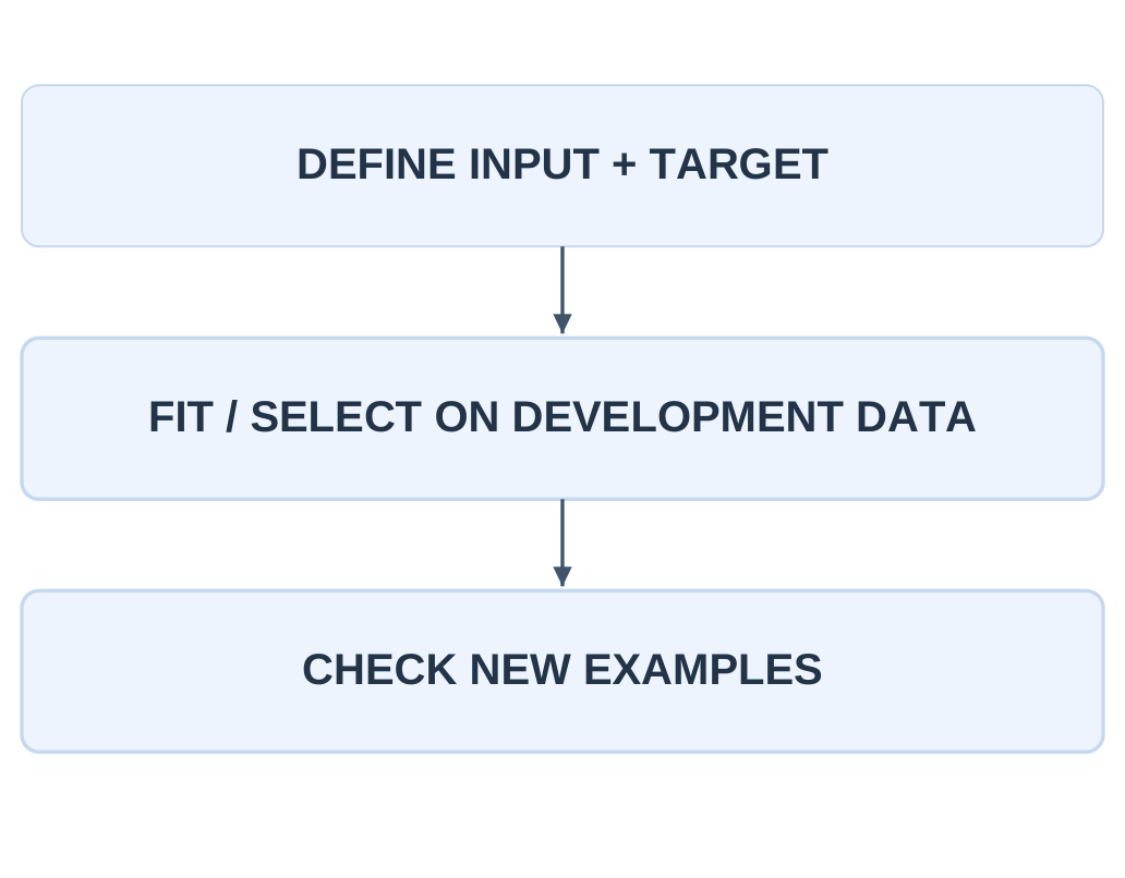
A learning workflow needs relevant data, consistent preprocessing, fitting or selection and a separate evaluation. Reusing development examples as the only check can reward memorization or a convenient collection pattern rather than useful generalization.

2.1.1 Methods Studied in This Unit
| Method | Learning Setup | Main Idea |
|---|---|---|
| KNN classifier | Supervised | Use nearby labelled examples |
| Naïve Bayes | Supervised | Compare class scores from probability estimates |
| K-Means | Unsupervised | Assign points to mean-based clusters |
| Neural network | Depends on objective | Learn weighted representations through layers |
KNN and K-Means both involve distance in their common forms, but they answer different questions. KNN uses known labels to predict a new label. K-Means discovers groups represented by centroids. Its cluster numbers are not pre-existing class names.
A numeric code can represent a category rather than a measured amount. Labels 0 and 1 for acceptable and defective define classification, even though numbers are used for storage.
2.1.2 Fair Comparison
- Use the same intended prediction-time information.
- Choose preprocessing using training information only.
- Use appropriate validation to choose settings.
- Compare final performance on held-out relevant examples.
- State what the selected measure counts and what it misses.
For example, predicting a known fault category from labelled past records is classification. Estimating hours of remaining operation is regression. Grouping unlabelled records by similarity is clustering.
The same source domain can support different tasks. The output and available feedback determine the learning problem.
2.2 K-Nearest Neighbors Classification
K-Nearest Neighbors (KNN) predicts a query’s class from nearby labelled training examples. In the simple uniform-vote version, select the k closest examples and give each one vote. The class with the most votes is predicted.
The choice of representation and distance determines what “nearby” means. A KNN classifier generally retains training examples rather than fitting one compact global formula in the introductory version. Prediction can therefore require substantial comparison work.
The value k is a chosen setting, not the number of classes. It must not exceed the available training examples. Distance ties and vote ties need a defined resolution policy.

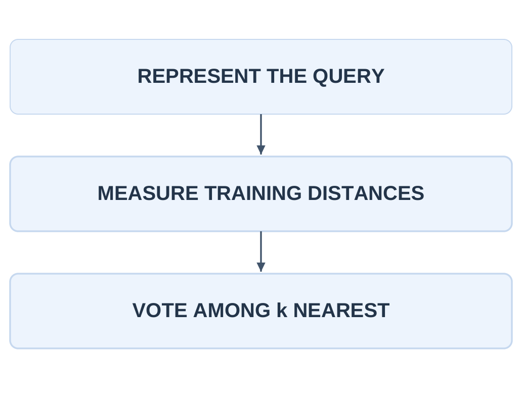
| Step | Action |
|---|---|
| 1 | Represent query and training inputs consistently |
| 2 | Calculate distances |
| 3 | Select k nearest training examples |
| 4 | Count votes and resolve any tie |
| 5 | Return the predicted category |
2.2.1 A Two-Feature Illustration

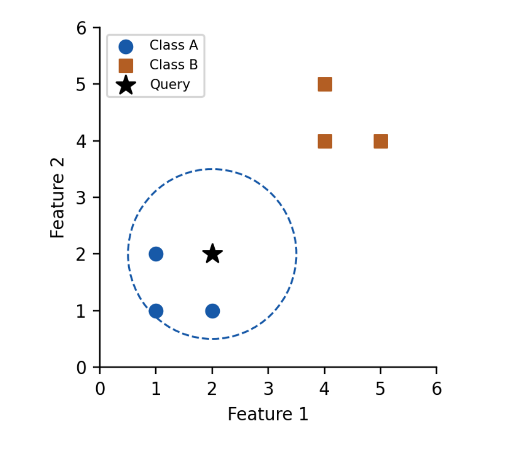
The Class A examples are (1,1), (1,2) and (2,1). Class B examples are (4,4), (4,5) and (5,4). The query is (2,2).
Under Euclidean distance, the three closest examples belong to A, so a uniform k = 3 vote predicts A.
The dashed circle illustrates the selected neighborhood. It is not a trained physical boundary. KNN’s prediction regions depend on all stored examples, the representation, distance and k.
2.2.2 What the Result Does Not Prove
A query far away from every known example can still receive a class under ordinary KNN. A confident-looking vote is not a guarantee that the query belongs to a well-represented situation.
Check whether the training distribution supports the intended use. There are two classes in the example, while k is three. These values do not conflict: class count describes possible labels; k describes how many neighbors participate in one prediction.
2.3 KNN: Distance and a Full Dry Run
For one numerical feature, absolute difference is a simple distance. For two features, Euclidean distance is the square root of the sum of squared coordinate differences. Both examples assume numerical features whose scales have been made meaningful.
For the point (2,2), the distance to (2,1) is 1; the distance to (1,1) is √2.
Taking the square root preserves the ordering of nonnegative squared distances, so a hand calculation can often compare squared values first.
Two-dimensional Euclidean distance
d = √[(x1 − q1)² + (x2 − q2)²]
Here x is a training point and q is the query. The same feature definitions must be used on both.
2.3.1 One-Feature Worked Example
Problem: Predict the class of query q = 3.2 using a uniform KNN classifier with k = 3.
| Training x | Class | Distance to q = 3.2 |
|---|---|---|
| 1 | A | 2.2 |
| 2 | A | 1.2 |
| 4 | B | 0.8 |
| 6 | B | 2.8 |
| 8 | B | 4.8 |
Step 1: Arrange the examples in ascending distance order.
4(B), 2(A), 1(A), 6(B), 8(B).
Step 2: Select the three nearest examples.
Selected labels: B, A, A.
Step 3: Count votes.
A receives two votes; B receives one vote.
Answer: The uniform k = 3 classifier predicts A.
Check: For k = 1, only 4(B) participates, so the prediction would instead be B.
Increasing k changes the neighborhood. A prediction need not remain the same when additional neighbors are included.
2.3.2 Scaling Affects Distance
| Feature | Possible Raw Scale | Issue |
|---|---|---|
| Temperature | 20–40 C | Tens of units |
| Rotational speed | 1000–5000 rpm | Thousands of units |
| Machine identifier | Digits naming a machine | Not a physical distance |
Without suitable preparation, a large numeric range can dominate distance even when the units do not justify that influence.
Scaling can help some distance-based comparisons, but it must be fitted using training information and applied consistently.
An identifier should not be treated as a meaningful quantity merely because it contains digits. Distance between arbitrary machine IDs says little about similarity of operation.
2.3.3 Ties and Weighting
For a query exactly at 3 between examples 2(A) and 4(B), the nearest-distance tie needs a policy.
An odd k helps avoid some two-class vote ties but does not prevent every tie, especially in multiclass settings.
A distance-weighted version gives more influence to nearer neighbors. It is a different prediction rule from the uniform vote used in the worked table.
State which rule is being applied before calculating an answer.
Practice check: For the same data and q = 7.5 with k = 3, the nearest examples are 8(B), 6(B) and 4(B), so the uniform vote predicts B.
2.4 Selecting k and Checking KNN
A very small k can make the classifier sensitive to an isolated erroneous or unusual example. A larger k averages over more neighbors but can smooth away meaningful local structure. There is no universally correct k for all datasets.
Choose k using a suitable validation process rather than repeatedly tuning it to a final test set. Keep the same permitted preprocessing in every comparison.
The test then assesses the chosen process instead of becoming a source of repeated design hints.
| Setting / Condition | Possible Consequence |
|---|---|
| k = 1 | Strong sensitivity to one nearest example |
| Larger k | Smoother vote; local minority can be outvoted |
| Irrelevant features | Distance becomes less useful |
| Unbalanced class counts | Large classes may dominate neighborhoods |
| Many stored examples | Prediction comparisons can be costly |
| New input far from training data | Class may be returned despite weak support |
2.4.1 Strengths
- Simple to explain with a labelled scatter plot.
- Naturally supports multiple classes through votes.
- Can model irregular class regions without one explicit linear boundary.
- Provides concrete neighboring examples that can be inspected.
Showing neighbors explains a particular vote, but it does not prove that the features or distance are appropriate, or that the examples are representative.
2.4.2 Small Engineering Example
Suppose labelled fabric patches are represented by a few meaningful texture features. A new patch can be compared with earlier patches using a chosen distance.
KNN supplies a category from the neighbors, while collection and representation determine whether that comparison is useful.
The original photographs should be separated into development and test groups before creating closely related crops. Otherwise near-duplicate patches can make evaluation unrealistically easy.
2.4.3 KNN Versus a Fixed Threshold
| Question | KNN | Manual Threshold |
|---|---|---|
| What defines the decision? | Stored examples, distance and k | Explicit rule chosen by designer |
| Does it use target labels? | Yes for the classifier | Not necessarily |
| Can new examples alter behavior? | Yes if stored reference set changes | Only if the rule changes |
| Is it automatically reliable? | No | No |
A simple threshold may be preferable when a known requirement directly defines the category.
KNN is useful when local similarity supplies a reasonable predictive basis. Complexity alone is not evidence of a better solution.
2.5 Naïve Bayes: Probability-Based Classification
Naïve Bayes is a family of supervised classifiers that compares class scores using Bayes’ theorem and a simplifying feature assumption.
It combines how common a class is with how compatible the observed features are with that class.
A prior probability expresses class frequency before the current feature evidence is considered.
A likelihood describes the probability of that evidence under a candidate class.
A posterior probability updates the class belief after considering the evidence.
Bayes’ theorem
P(C | X) = P(X | C) × P(C) / P(X)
C is a class and X is the observed feature vector. For comparing classes for the same X, the denominator P(X) is common and may be omitted from the scores when the comparison is defined.

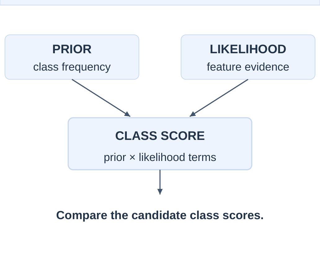
The largest unnormalized score gives the same selected class as the corresponding normalized scores, provided the denominator is positive.
A score by itself is not yet a probability that sums to one across classes.
2.5.1 What Makes It “Naïve”?
The model assumes that features are conditionally independent given the class.
It approximates the joint likelihood by multiplying individual feature likelihoods. This does not mean that all features are independent in the original population.
For features x1 and x2, the introductory class score is:
Score(C) = P(C) × P(x1 | C) × P(x2 | C)
The same idea extends to additional features. The assumption reduces the amount of probability information that must be estimated.
| Quantity | Meaning in a Spam Example |
|---|---|
| P(Spam) | Prior proportion of spam messages |
| P(urgent = 1 | Spam) | Chance that urgent appears among spam |
| P(link = 1 | Spam) | Chance that a link appears among spam |
| P(Spam | features) | Updated class probability under the model |
2.5.2 Why Use the Assumption?
Without a simplifying model, every combination of many features could require its own estimate. With limited examples, most combinations may be rare or unseen.
Naïve Bayes uses smaller sets of estimates, which can make fitting and prediction efficient.
Real features are often related. Words can occur together and sensor measurements can be correlated. The method can still be useful, but its assumptions and evaluation must be discussed.
Exam wording: “Features are conditionally independent given the class” is the required assumption. Writing only “all inputs are unrelated” changes its meaning.
2.6 Naïve Bayes: A Numerical Example
Consider ten labelled messages: four spam and six legitimate.
Two binary features indicate whether the word urgent and a link occur. A value of 1 means present and 0 means absent.
These are synthetic teaching records, not a recommended production spam dataset.
| Class | Feature Pairs (urgent, link) |
|---|---|
| Spam: 4 | (1,1), (1,1), (1,0), (0,1) |
| Legitimate: 6 | (1,0), (0,1), (0,1), (0,0), (0,0), (0,0) |
2.6.1 Estimate Priors and Likelihoods
| Estimate | Spam | Legitimate |
|---|---|---|
| Class prior | 4/10 | 6/10 |
| urgent = 1 | 3/4 | 1/6 |
| link = 1 | 3/4 | 2/6 |
The denominator for each feature likelihood is the number of training records in that class.
For example, urgent occurs in three of the four spam messages:
P(urgent = 1 | Spam) = 3/4
Do not divide that count by ten: 3/10 is a different probability.
Conditional probabilities use the class-specific group specified after the vertical bar.
Query: The new message has urgent = 1 and link = 1. Compare both candidate class scores using those same observed feature values.
2.6.2 Calculate the Scores
Spam score
Score(Spam) = (4/10) × (3/4) × (3/4)
Score(Spam) = 0.225
Legitimate score
Score(Legitimate) = (6/10) × (1/6) × (2/6)
Score(Legitimate) = 0.03333…
Answer: The spam score is larger, so the unsmoothed Naïve Bayes classifier predicts Spam.
The common evidence denominator is unnecessary for this class comparison.
2.6.3 Optional Normalization
The sum of scores is:
0.225 + 0.03333… = 0.25833…
The normalized spam score is:
0.225 / 0.25833… = 27/31 ≈ 0.871
The normalized legitimate score is:
4/31 ≈ 0.129
They sum to one under this fitted model.
This 0.871 follows from the chosen model, features and tiny synthetic sample. It does not establish an 87.1% real-world success rate or guarantee that this message is spam.
| Check | Answer |
|---|---|
| How many candidate classes? | Two |
| Do query labels enter prediction? | No |
| Which score is larger? | Spam |
| Are scores based on true joint counts? | No; likelihood product uses the naïve assumption |
| Does normalization change the winner? | No |
2.7 Naïve Bayes: Smoothing and Limits
If a feature value was never seen in a class, an unsmoothed likelihood estimate can be zero.
Multiplying it into a class score makes the whole score zero, even when other observed features support that class. A small training sample can therefore produce overly absolute exclusions.
Laplace smoothing adds one to each possible feature-value count.
For a binary feature within a class, the denominator increases by two because that feature has two possible values. Apply the chosen estimation rule consistently.
Binary Laplace estimate
P(x = v | C) = (count of v in class C + 1) / (number of class-C examples + 2)
This formula applies to the binary feature setup used here. Other Naïve Bayes variants estimate different distributions.
2.7.1 Apply It to the Previous Data
| Likelihood | Spam | Legitimate |
|---|---|---|
| urgent = 1 | (3+1)/(4+2) = 4/6 | (1+1)/(6+2) = 2/8 |
| link = 1 | (3+1)/(4+2) = 4/6 | (2+1)/(6+2) = 3/8 |
Keeping the earlier class priors:
Smoothed Spam score
0.4 × (4/6) × (4/6) ≈ 0.17778
Smoothed Legitimate score
0.6 × (2/8) × (3/8) = 0.05625
Answer: Spam still wins, but the estimates have changed.
Smoothing reduces zero-frequency problems. It does not remove dependence between features, repair misleading labels or prove that probabilities are calibrated.
2.7.2 Common Variants
| Variant | Typical Feature Interpretation |
|---|---|
| Bernoulli | Binary indicators such as presence / absence |
| Multinomial | Nonnegative count-style text features |
| Gaussian | Continuous features modelled with class-specific Gaussian distributions |
Do not apply the binary count formula blindly to a continuous temperature value.
The data representation and distribution assumption determine the appropriate likelihood model.
The common principle is prior times an approximated class-conditional likelihood.
2.7.3 Strengths and Limitations
- Often quick to fit and predict with simple feature estimates.
- Can provide a useful text-classification baseline.
- Needs labelled examples for the classification task.
- Related or redundant features can distort evidence.
- Unseen distributions and poor labels can reduce reliability.
- High model scores should be checked against held-out outcomes.
2.7.4 Compare with KNN
KNN relies on distances to stored labelled examples.
Naïve Bayes relies on estimated class priors and likelihoods.
A numeric feature range directly affects an ordinary Euclidean KNN distance. Naïve Bayes instead needs a suitable probability model for the feature.
Neither method is always superior.
2.8 K-Means Clustering
K-Means is an unsupervised method that groups numerical examples into k clusters.
Each cluster is represented by a centroid: the arithmetic mean of its assigned points.
The usual method alternates between assigning points and updating these means.
In standard K-Means, each point is assigned to a nearest centroid under Euclidean distance. The fitting objective is to reduce the sum of squared distances from points to their assigned centroids.
The method does not receive the target category of every training point.

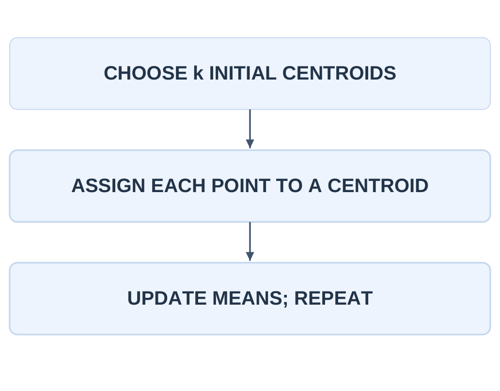
2.8.1 Algorithm Steps
Step 1: Choose k and initialize k centroid positions.
Step 2: Assign each point to a nearest centroid.
Step 3: Replace each centroid by the mean of its assigned points.
Step 4: Repeat assignment and update until assignments stabilize or another stopping rule is met.
2.8.2 Interpreting a Centroid
For a one-feature cluster {1, 2, 4}:
Centroid = (1 + 2 + 4)/3 = 7/3
It need not equal any observed value.
In two dimensions, take the mean of each coordinate separately.
Cluster numbers such as 0 and 1 are identifiers, not quality ranks or confirmed semantic classes.
Interpreting a group as a machine regime or fabric type requires further evidence.
| KNN Classification | K-Means Clustering |
|---|---|
| Uses known target labels | Uses unlabelled inputs for clustering |
| k counts neighbors in a vote | k counts clusters / centroids |
| Predicts a category from neighbors | Fits groups by assignment and mean update |
| Training examples provide labels | Centroids summarize assigned coordinates |
2.8.3 Distance Still Needs Preparation
A large-scale numerical feature can dominate squared distances. Use meaningful units and suitable scaling when needed.
Arbitrary identifiers should not be treated as measured coordinates.
K-Means is especially suited to compact groups under the selected geometry. Long curved groups, unequal spread or strong outliers can lead to misleading partitions.
A visible grouping is a hypothesis to assess, not a discovered law.
Important distinction: Setting k = 3 instructs the algorithm to fit three centroids. It does not prove that the data contains exactly three natural categories.
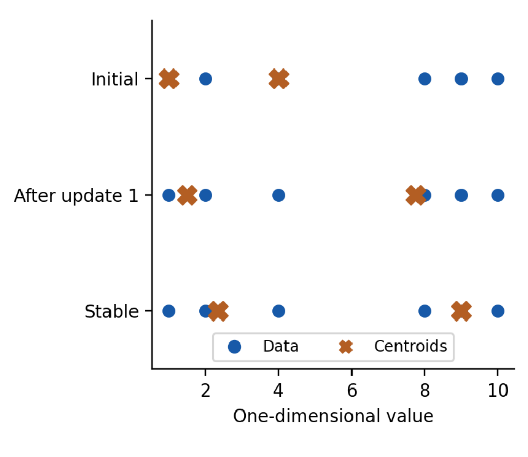
2.9 K-Means: Complete Numerical Dry Run
Take the one-dimensional data:
{1, 2, 4, 8, 9, 10}
Choose k = 2 with initial centroids:
c1 = 1 and c2 = 4
This simple initialization makes the repeated assignment-and-update process visible. No target labels are supplied.
2.9.1 First Assignment
| Point | Distance to 1 | Distance to 4 | Assigned |
|---|---|---|---|
| 1 | 0 | 3 | C1 |
| 2 | 1 | 2 | C1 |
| 4 | 3 | 0 | C2 |
| 8 | 7 | 4 | C2 |
| 9 | 8 | 5 | C2 |
| 10 | 9 | 6 | C2 |
The first groups are:
C1 = {1, 2}
C2 = {4, 8, 9, 10}
For this one-dimensional assignment, ordinary absolute distances give the same nearest-centroid choice as squared distances.
2.9.2 First Mean Update
c1 = (1 + 2)/2 = 1.5
c2 = (4 + 8 + 9 + 10)/4 = 31/4 = 7.75
The point 4 was initially a centroid, but that does not permanently bind it to that cluster.
Centroids move after the mean update; assignments are then recalculated.
Complete the assignment using the current centroids, then calculate the new means. Do not move a centroid after every individual point in this batch K-Means example.
2.9.3 Second Assignment and Update
| Point | Distance to 1.5 | Distance to 7.75 | Assigned |
|---|---|---|---|
| 1 | 0.5 | 6.75 | C1 |
| 2 | 0.5 | 5.75 | C1 |
| 4 | 2.5 | 3.75 | C1 |
| 8 | 6.5 | 0.25 | C2 |
| 9 | 7.5 | 1.25 | C2 |
| 10 | 8.5 | 2.25 | C2 |
Now:
C1 = {1, 2, 4}
C2 = {8, 9, 10}
The new centroids are:
c1 = (1 + 2 + 4)/3 = 7/3 ≈ 2.333
c2 = (8 + 9 + 10)/3 = 9
A further assignment leaves these groups unchanged, so the example has stabilized.
2.9.4 Check the Final Objective
For C1, squared deviations from 7/3 are:
16/9, 1/9 and 25/9
Their total is:
42/9 = 14/3
For C2, squared deviations from 9 are:
1, 0 and 1
Their total is 2.
The final within-cluster sum of squares is:
14/3 + 2 = 20/3 ≈ 6.667
This calculation uses squared deviations, not the unsquared distances shown for assignment.
Exam check: Show initialization, assignment distances, cluster memberships, new means and a stopping check. Naming only the final groups does not demonstrate the algorithm.
2.10 Assessing K-Means Results

Different starting centroids can produce different local solutions. Repeating fitting with appropriate initializations can help, but it does not prove that a universally best grouping has been found.
State the initialization when doing a hand calculation.
An empty cluster has no ordinary arithmetic mean of assigned points. A complete implementation needs a policy, such as reinitializing that centroid.
Introductory examples often avoid the case, but that does not make it impossible.
2.10.1 Choosing k
Choosing more clusters generally reduces the fitted within-cluster squared distance.
That reduction alone does not justify making every point its own cluster. Consider usefulness, stability and appropriate validation.
An elbow plot looks for a change in how much the objective improves as k increases.
The bend can be unclear. It is a heuristic rather than an automatic discovery of the true class count.
2.10.2 Practical Failure Cases
| Condition | Why Interpretation Can Fail |
|---|---|
| Unequal feature units | A large range dominates distance |
| Extreme outlier | The mean can move substantially |
| Curved or noncompact groups | Nearest-centroid partitions may not match shape |
| Wrong chosen k | Distinct patterns may merge or one pattern may split |
| Duplicate / biased collection | Groups can reflect the collection process |
2.10.3 A Fabric-Inspection Example
Suppose unlabelled fabric patches are represented by brightness and texture measurements.
K-Means can divide them into similarity groups. One group might later be inspected and found to contain many defects.
It would still be incorrect to call the original fit supervised defect classification. The clustering algorithm did not receive defect labels.
Human review and a later labelled prediction system are separate steps.
Use samples from different rolls and conditions when checking meaning. If all dark images form one group, that may describe lighting rather than a useful material difference.
2.10.4 Quick Comparison Check
For KNN, a new query inherits a label from nearby known examples.
For K-Means, a point can be assigned to a fitted nearest centroid, but that cluster ID has no guaranteed class meaning.
Keep the two uses of k separate throughout your answer.
2.11 Evaluating a Classifier
A classification metric summarizes predicted categories against known reference outcomes.
Begin by defining the positive class. Otherwise terms such as false positive are ambiguous.
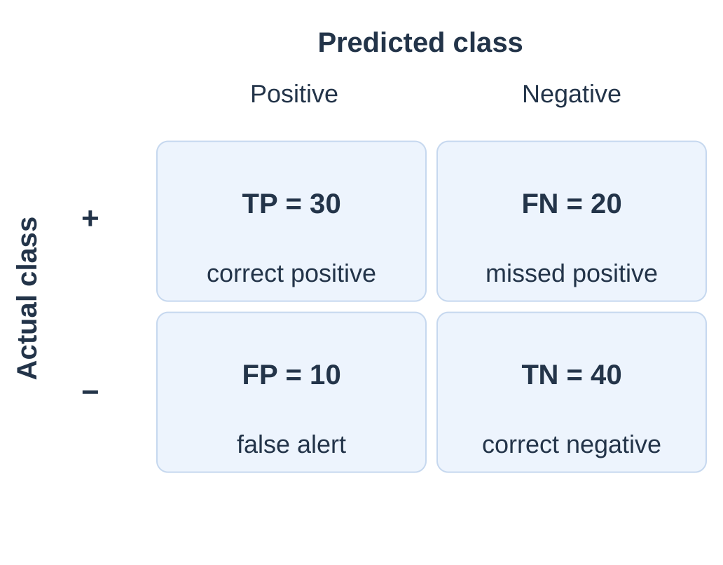
In this example, positive means “needs inspection.”
A true positive (TP) is an inspection-needed case predicted positive.
A false positive (FP) is a normal case incorrectly flagged.
A false negative (FN) is an inspection-needed case incorrectly missed.
A true negative (TN) is a normal case correctly left negative.

| Count | Practical Interpretation |
|---|---|
| TP = 30 | Correctly flagged inspection cases |
| FP = 10 | Unnecessary flags |
| FN = 20 | Missed inspection cases |
| TN = 40 | Correctly unflagged normal cases |
2.11.1 Read the Matrix Correctly
The actual positive count is:
TP + FN = 30 + 20 = 50
The predicted positive count is:
TP + FP = 30 + 10 = 40
These are different totals.
A question about all real positives uses the first denominator. A question about all predicted positives uses the second.
The total is:
30 + 10 + 20 + 40 = 100
Correct outcomes are:
TP + TN = 70
Incorrect outcomes are:
FP + FN = 30
Both row totals and column totals should sum to the same overall number.
2.11.2 Why One Score Is Not Enough
Accuracy combines correct predictions from both classes.
Precision asks how trustworthy the positive flags were.
Recall asks how many actual positives were found.
F1 balances precision and recall through their harmonic mean.
The preferred measure depends on the task. Unnecessary inspection consumes effort, while a missed defect may have a different consequence.
State the relevant error instead of claiming that one metric is best for every application.
| Question | Relevant Measure |
|---|---|
| How often are all predictions correct? | Accuracy |
| How many positive flags are correct? | Precision |
| How many actual positives are found? | Recall |
| How can precision and recall be combined? | F1 score |
Some books exchange rows and columns in confusion matrices. Read the labels before placing TP, FP, FN and TN.
The definitions refer to actual and predicted outcomes, not a memorized position on the page.
2.12 Accuracy, Precision, Recall and F1
2.12.1 Accuracy
Formula
Accuracy = (TP + TN) / (TP + TN + FP + FN)
Worked calculation
Accuracy = (30 + 40)/100
Accuracy = 0.70 = 70%
Accuracy gives the fraction of all cases classified correctly.
It can be useful when the evaluation population and error priorities are suitable, but it hides how errors are divided between classes.
2.12.2 Precision
Formula
Precision = TP / (TP + FP)
Worked calculation
Precision = 30/(30 + 10)
Precision = 0.75 = 75%
Among forty positive flags, thirty were correct.
High precision means relatively few false positive flags compared with the number of positive flags.
It does not tell us how many real positives were missed.
2.12.3 Recall
Formula
Recall = TP / (TP + FN)
Worked calculation
Recall = 30/(30 + 20)
Recall = 0.60 = 60%
Among fifty actual positives, thirty were found. The other twenty are false negatives.
High recall means few misses relative to the actual positive count. It does not alone describe the reliability of all generated flags.
2.12.4 F1 Score
Equivalent formulas
F1 = 2 × precision × recall / (precision + recall)
F1 = 2TP / (2TP + FP + FN)
Worked calculation
F1 = 60/(60 + 10 + 20)
F1 = 2/3 ≈ 0.667
F1 is the harmonic mean of precision and recall.
It becomes low when one of them is low and does not include TN directly in its binary count formula.
It is not simply the arithmetic average of 0.75 and 0.60.
Using the first form:
F1 = 2 × 0.75 × 0.60 / 1.35
F1 ≈ 0.6667
The arithmetic average would be 0.675, which is a different calculation.
| Measure | Value | Main Interpretation |
|---|---|---|
| Accuracy | 0.70 | 70 of 100 cases correct |
| Precision | 0.75 | 30 of 40 flags correct |
| Recall | 0.60 | 30 of 50 positives found |
| F1 | 0.667 | Harmonic balance of precision and recall |
2.12.5 Denominator Checks
If there are no predicted positives, precision has a zero denominator.
If there are no actual positives, recall has a zero denominator.
A reporting system may choose a stated convention, such as displaying zero in some cases, but the raw fraction is undefined.
Always state percentages or fractions consistently. Do not mix precision 75 with recall 0.60 in the same formula without converting them to a consistent scale.
Memory aid: Precision starts with the predicted-positive group. Recall starts with the real-positive group.
2.13 Imbalance and Decision Thresholds
Suppose a test set contains ninety-five negatives and five positives.
A classifier that predicts negative for everyone has 95% accuracy.
Its counts are:
TP = 0, FN = 5, FP = 0, TN = 95
Its recall is zero.
Its precision fraction is 0/0, which is undefined. An implementation may report a conventional zero if that rule is explicitly chosen.
High accuracy therefore does not prove that a rare positive class is being found.
2.13.1 Scores Versus Decisions
Some classifiers produce a positive-class score. A threshold converts that score to a category.
In this example:
Predict positive when score ≥ threshold.
Raising the threshold produces fewer or the same number of positive flags for the same fixed scores.
| Case | Actual | Score | At 0.5 | At 0.7 |
|---|---|---|---|---|
| A | 1 | 0.90 | 1 | 1 |
| B | 1 | 0.60 | 1 | 0 |
| C | 0 | 0.55 | 1 | 0 |
| D | 0 | 0.10 | 0 | 0 |
At threshold 0.5:
TP = 2, FP = 1, FN = 0, TN = 1
At threshold 0.7:
TP = 1, FP = 0, FN = 1, TN = 2
The model scores have not changed; the decision rule has.
Choose the operating threshold using development evidence and task needs. Repeatedly choosing it to maximize the final test score weakens that test’s independence.
2.13.2 Compare Both Operating Points
| Metric | Threshold 0.5 | Threshold 0.7 |
|---|---|---|
| Accuracy | 3/4 = 0.75 | 3/4 = 0.75 |
| Precision | 2/3 ≈ 0.667 | 1/1 = 1.00 |
| Recall | 2/2 = 1.00 | 1/2 = 0.50 |
| F1 | 4/5 = 0.80 | 2/3 ≈ 0.667 |

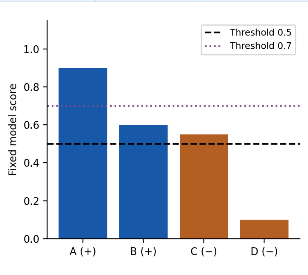
Both settings have the same accuracy, but different errors.
The stricter setting has perfect precision in this tiny example while missing one of the two real positives.
A metric comparison should name that practical change.
A score need not be a well-calibrated probability. Treat 0.90 as a model score unless its probability interpretation has been established.
More decimal places do not guarantee better evidence.
These formulas concern a defined binary positive class. Multiclass reporting needs stated class-wise comparisons and averaging rules.
2.14 Mean Absolute Error: Numerical Prediction
Mean Absolute Error (MAE) measures the average magnitude of numerical prediction errors.
It belongs to regression evaluation. The syllabus places it beside classification measures, but accuracy, precision, recall and F1 answer different questions.
For each example:
- Subtract the actual value from the predicted value.
- Take the absolute magnitude.
- Average across examples.
Absolute values prevent positive and negative errors from cancelling.
Formula
MAE = (1/n) × sum of |predicted value − actual value|
MAE ≥ 0, with zero meaning exact predictions on the evaluated examples.
| Actual | Predicted | Signed Error | Absolute Error |
|---|---|---|---|
| 10 | 12 | +2 | 2 |
| 20 | 18 | −2 | 2 |
| 30 | 33 | +3 | 3 |
| 40 | 37 | −3 | 3 |
Worked calculation
MAE = (2 + 2 + 3 + 3)/4
MAE = 10/4 = 2.5
If these values are durations in minutes, MAE is 2.5 minutes. The result retains the units of the target variable.
The mean signed error is:
(2 − 2 + 3 − 3)/4 = 0
That zero hides substantial individual errors. It describes cancellation rather than exact prediction.
2.14.1 Interpretation and Limits
MAE describes a typical absolute error magnitude across the supplied cases.
It does not indicate whether predictions are mostly too high or too low, and it does not describe the largest error.
Additional checks can be needed for the task.
An MAE of 2.5 has different significance for a process tolerance of 0.1 than for a target naturally varying by hundreds of units.
Interpret the value with target units, a useful baseline and the evaluation conditions.
| Question | Suitable Approach |
|---|---|
| Acceptable or defective? | Classification metrics |
| Predicted energy in kWh? | MAE can assess numerical errors |
| Average absolute temperature error? | MAE in temperature units |
| Are positive flags usually correct? | Precision |
| Are actual defects being missed? | Recall |
2.14.2 Do Not Average Arbitrary Label Codes
Coding three unordered classes as 0, 1 and 2 does not make their differences meaningful numerical distances.
MAE on such codes changes when the codes are reassigned, even though the categories are unchanged.
For regression, compare models on the same target and comparable held-out examples.
A lower test MAE can indicate better numerical predictions under those conditions, but it does not prove reliability in a different operating environment.
Exam correction: If asked to list classification metrics including MAE, give the requested formula and explicitly identify MAE as a regression error measure.
2.15 Artificial Neurons
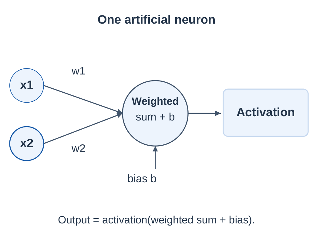
An artificial neuron combines input values using learnable weights, adds a bias and applies an activation function.
It is a mathematical computing unit inspired loosely by biological ideas. It is not a full simulation of a human nerve cell.
For inputs x1 and x2:
z = w1x1 + w2x2 + b
The output is:
a = f(z)
Here f is the activation function.
A network links many such units so that one layer’s outputs become inputs to another.

| Component | Role |
|---|---|
| Input x | A supplied feature or earlier-layer output |
| Weight w | Controls contribution of an input |
| Bias b | Adds an adjustable offset |
| Activation f | Transforms the weighted input |
| Output a | Value passed onward |
2.15.1 One Neuron: Worked Calculation
Given
x1 = 2
x2 = 1
w1 = 0.5
w2 = −1
b = 0.2
Step 1: Compute the weighted input
z = (0.5 × 2) + (−1 × 1) + 0.2
z = 1 − 1 + 0.2
z = 0.2
Step 2: Apply ReLU
ReLU(z) = max(0,z)
a = max(0,0.2) = 0.2
Answer: The neuron output is 0.2.
If x2 becomes 2 while other values remain unchanged:
z = 1 − 2 + 0.2 = −0.8
ReLU(−0.8) = 0
A negative weighted input does not produce a negative ReLU output.
2.15.2 Interpreting Weights Carefully
A positive weight raises z when that input increases with everything else fixed. A negative weight lowers it.
The practical meaning also depends on feature units, preprocessing and interactions in later layers.
A larger weight magnitude does not automatically prove that a feature is causally important.
Rescaling a feature changes the corresponding weight needed for the same weighted sum.
2.15.3 Bias Versus Input
The bias is a learned offset added after the weighted feature contributions.
It allows a neuron’s response to shift even when all supplied input values are zero.
It is not the same concept as unfairness in a social or data-bias discussion.
The network learns parameter values through a training procedure and objective.
Writing down a neuron equation specifies a computation; it does not by itself explain how useful weights were obtained.
2.16 Layers and Network Structure
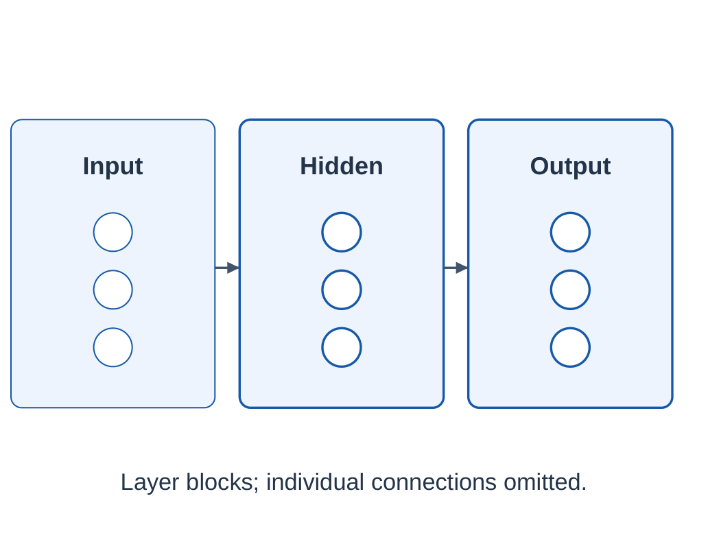
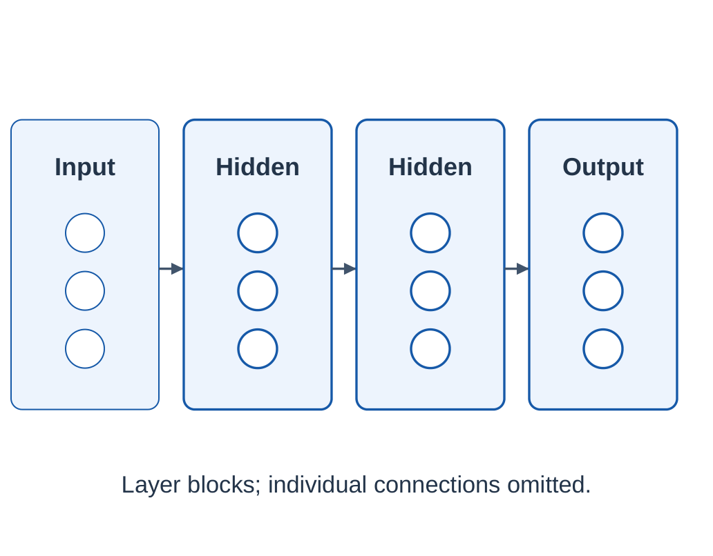
A neural network organizes connected computational units into layers.
The input layer represents the supplied features.
Hidden layers transform intermediate representations.
The output layer supplies values appropriate to the task.
A fully connected layer allows every unit in that layer to use all outputs from the preceding layer.
Other architectures use more selective connections, as convolutional layers do for local image patterns.

2.16.1 Feedforward Calculation
In a feedforward network, compute each layer from earlier-layer values and pass the outputs onward.
For one example, the forward calculation ends at a prediction or score.
Training uses that result to assess error and adjust parameters.
Two hidden layers can represent successive transformations. Their representations are learned numbers; they do not automatically correspond to familiar human concepts or words.
Width and depth
Width concerns the number of units in a layer.
Depth concerns the number of successive processing layers.
A wider shallow network and a narrower deep network are different structures.
2.16.2 Output Depends on the Task
| Task | Possible Output Arrangement |
|---|---|
| Binary classification | One positive-class score, with a stated decision threshold |
| Multiclass classification | One score per category, often normalized with softmax |
| Regression | One or more numerical target predictions |
A network output of 0.7 does not identify the class unless the task, score meaning and decision rule are known.
The output layer and training objective must match the target.
For a three-category classifier, the categories might be acceptable, stain and tear.
Three output scores can be compared to select a category, but this does not mean that the input contains only three features.
2.16.3 Count a Small Layer’s Parameters
A fully connected layer with two inputs and three neurons has:
Weights = 2 × 3 = 6
With one bias per neuron:
Biases = 3
Total trainable parameters = 6 + 3 = 9
If those three outputs feed a single output neuron, the next layer adds:
Weights = 3
Biases = 1
Additional parameters = 4
The two-layer calculation therefore has:
9 + 4 = 13 trainable parameters
Input features, neurons, layers and parameters count different things.
An input layer that merely supplies feature values does not itself add another set of learned weights.
2.17 Activation and Representation Learning
An activation function transforms a neuron’s weighted input.
Nonlinear activations allow a network to represent functions that cannot be achieved by simply collapsing a sequence of ordinary linear transformations into one.
If every layer applies only an affine transformation, stacking them still produces one overall affine transformation.
Extra layers then do not supply the same nonlinear representational benefit.

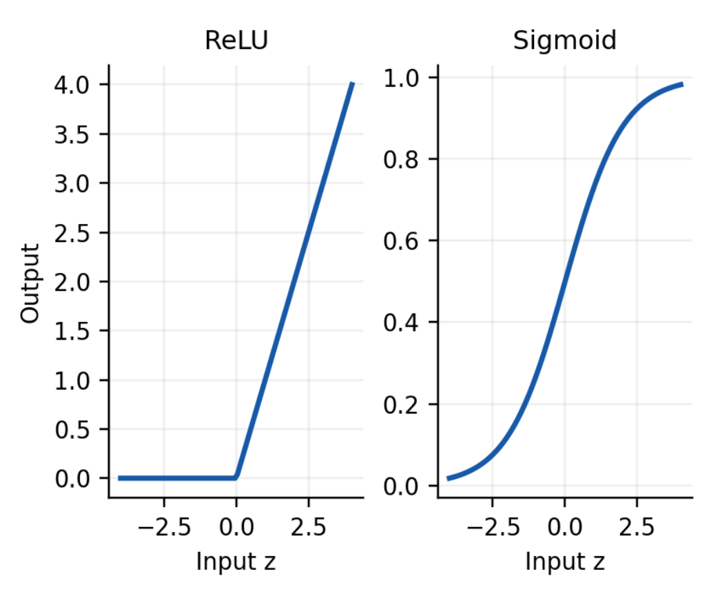
| Activation | Basic Expression / Behavior |
|---|---|
| ReLU | max(0,z) |
| Sigmoid | 1 / (1 + exp(−z)) |
| Linear output | Returns z directly |
The activation choice depends on where the layer is used and what output is needed.
A linear output can be suitable for unrestricted numerical prediction; a sigmoid output can supply a binary score.
No single activation is required at every position.
2.17.1 Features Supplied and Features Learned
A traditional model may receive carefully designed input measurements, such as texture summaries from an image.
A neural network can learn intermediate transformations while optimizing its target task.
The initial input preparation still matters.
For an image, an early convolutional layer may respond to local patterns. Later transformations combine information across larger regions.
This is an explanatory tendency, not a promise that every unit corresponds to a named object part.
2.17.2 Historical Connections

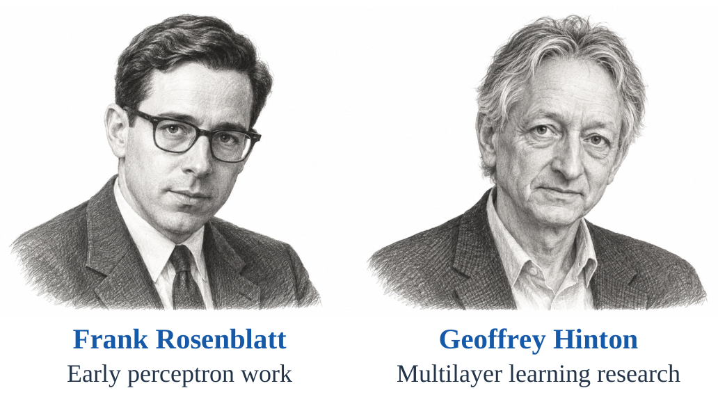
Frank Rosenblatt’s perceptron work helped establish early trainable neural classifiers.
A single-layer linear-threshold perceptron has important representational limits, including the usual XOR example.
Geoffrey Hinton contributed to multilayer neural-network learning and later deep-learning research.
Backpropagation was developed through contributions from multiple researchers. It should not be credited to one scientist alone.
Modern neural systems differ greatly in architecture and scale.
These portraits provide historical anchors for trainable weighted units and learning through multiple layers. They do not imply that today’s systems are direct copies of one early model.
2.18 How Network Training Changes Weights
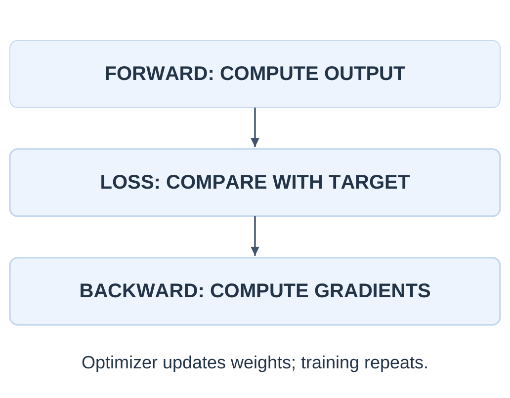
Training seeks parameter values that reduce a chosen loss on training examples.
A forward pass produces model outputs.
The loss compares outputs with targets according to the task.
Backpropagation computes derivatives that describe how the loss changes with parameters.
An optimizer uses those derivatives to update weights and biases.
Backpropagation computes gradient information; the optimizer performs the update. The two are related steps, not interchangeable names for the entire training process.

2.18.1 A Tiny Update Example
Given
Current weight w = 0.50
Computed loss gradient = +0.20
Learning rate = 0.10
Simple gradient-descent rule
w_new = w − learning rate × gradient
Substitution
w_new = 0.50 − 0.10 × 0.20
w_new = 0.48
Answer: The updated weight is 0.48.
A negative gradient would move the weight upward under this rule.
A gradient is a local direction signal, not a target class or a distance to a training example.
A very large learning rate can overshoot useful regions. A very small rate can make learning slow.
2.18.2 Epochs, Batches and Generalization
| Term | Meaning |
|---|---|
| Batch | Examples used together for an update or computation |
| Epoch | One pass through the chosen training dataset |
| Loss | Objective quantity used to guide fitting |
| Validation | Development check used for selection |
| Inference | Using fixed learned parameters to produce an output |

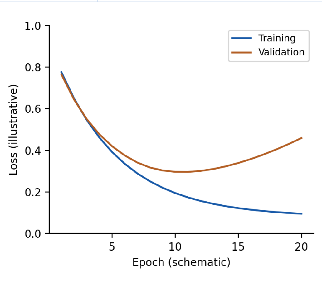
Lower training loss alone does not establish better performance on new examples.
Overfitting occurs when learned behavior matches training-specific details that do not generalize well.
Use appropriate held-out data, a suitable model size and other justified training controls.
Once selection is complete, an independent test gives a more useful assessment than a repeatedly consulted development set.
Ordinary inference does not necessarily update weights.
2.19 Deep Learning and GPU Acceleration
Deep learning uses neural networks with multiple processing layers to learn representations for a task.
There is no single universal layer-count cutoff that makes every architecture deep.
The important idea is successive learned transformations.
Depth can support hierarchical representations, but a deeper network is not automatically more accurate.
Useful training also depends on appropriate architecture, optimization, data, compute and evaluation.

2.19.1 Why Computation Grows
Training repeatedly performs matrix multiplications and related array operations across examples, parameters and layers.
Large images, many examples or wide layers can increase computational and memory requirements.
A model’s needs depend on its actual size and workload.
A small neural network can be trained on a CPU. It is incorrect to say that every deep-learning experiment requires a GPU.
Adding layers, data or compute without addressing the real task can increase cost while leaving collection or evaluation problems unresolved.
2.19.2 Why GPUs Are Useful

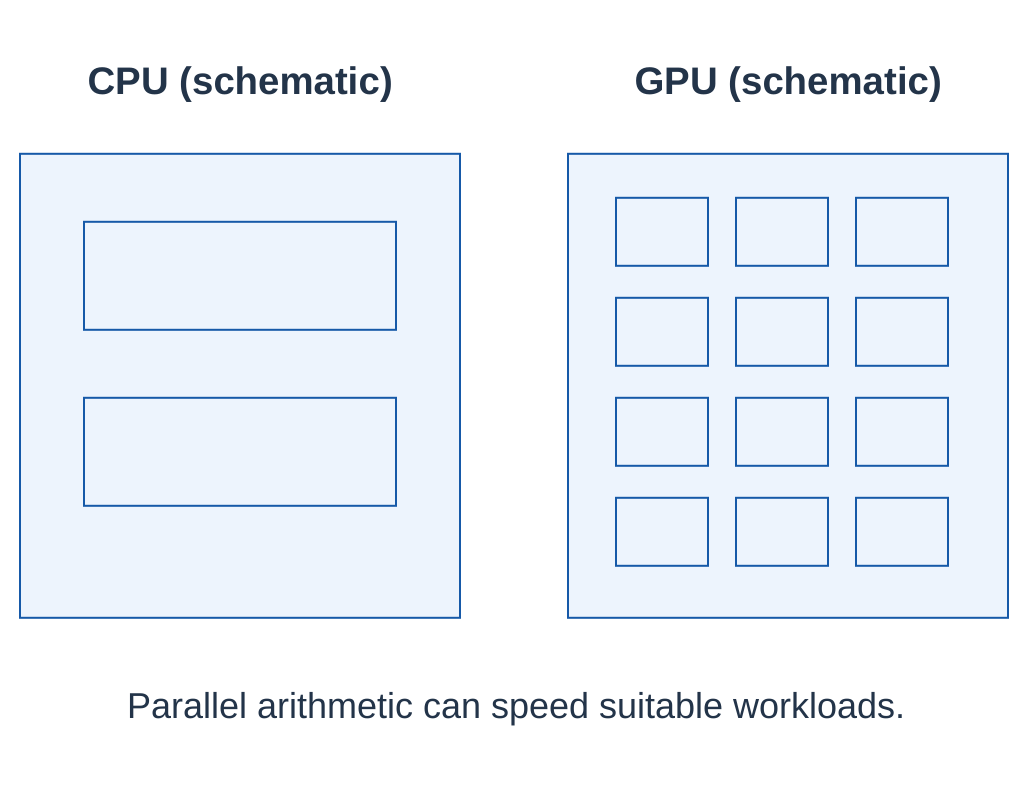
A Graphics Processing Unit (GPU) can execute many suitable arithmetic operations in parallel.
Dense matrix and tensor computations often expose the kind of parallel work that GPUs can accelerate.
Specialized libraries organize these operations efficiently.
A CPU remains important for general program control, data preparation and tasks that do not map well to a GPU.
Moving data between memories and fitting arrays into available memory can affect total speed.
A GPU does not select correct labels or make a biased dataset representative.
Faster computation accelerates the supplied procedure; it does not establish its validity.
| Consideration | Question to Ask |
|---|---|
| Parallel workload | Can operations be performed together? |
| Memory | Do data and model fit? |
| Transfer overhead | Does movement outweigh saved computation? |
| Scale | Is a CPU already sufficient? |
2.20 Convolutional Neural Networks
A Convolutional Neural Network (CNN) uses learned local filters to process spatially arranged data such as images.
The same filter parameters are applied at different image positions. This weight sharing makes a filter reusable across locations.
A small filter examines a local neighborhood, multiplies corresponding values and combines the results.
Sliding the filter produces a feature map.
A CNN learns filter values during training rather than requiring a person to design every useful pattern detector.

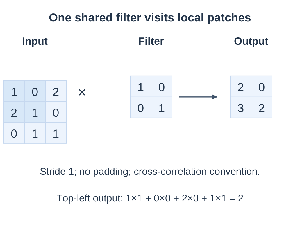
2.20.1 Read One Output Cell
Input
[[1,0,2], [2,1,0], [0,1,1]]
Filter
[[1,0], [0,1]]
Settings
Stride = 1
Padding = 0
The filter is not flipped.
The upper-left input patch is:
[[1,0], [2,1]]
Multiply corresponding values and add:
1×1 + 0×0 + 2×0 + 1×1 = 2
Moving one column right uses:
[[0,2], [1,0]]
This gives:
0×1 + 2×0 + 1×0 + 0×1 = 0
Repeat on the lower two patches.
Output feature map
[[2,0], [3,2]]
This example has no additional bias or activation.
2.20.2 Locality and Weight Sharing
A fully connected image layer would assign separate connections to many pixel positions.
A convolutional filter uses a small local region and shares its weights across positions.
One filter therefore tests a related pattern throughout the input.
Different learned filters can respond to different patterns.
A feature map contains the responses of one filter across spatial locations. Multiple filters can produce multiple feature channels.
| Term | Meaning |
|---|---|
| Kernel / filter | Small learned array used locally |
| Feature map | Spatial output of the filter operation |
| Stride | Movement between filter positions |
| Padding | Extra border values used during the operation |
| Channel | One component of the representation, such as an input color component |
2.20.3 Stride and Output Size
For one spatial dimension:
Output size = floor((N + 2P − F)/S) + 1
Where:
- N = input size
- F = filter size
- P = padding
- S = stride
The settings must define valid filter positions.
In the worked example:
N = 3, F = 2, P = 0 and S = 1
Output size = floor((3 − 2)/1) + 1
Output size = 2
The output is therefore two by two.
A larger stride samples fewer filter positions. Padding can help control spatial size and border treatment.
Terminology detail: Strict mathematical convolution flips the filter. Common CNN layers use the unflipped cross-correlation shown here. State the operation used in a numerical answer.
2.21 Pooling and a CNN Pipeline
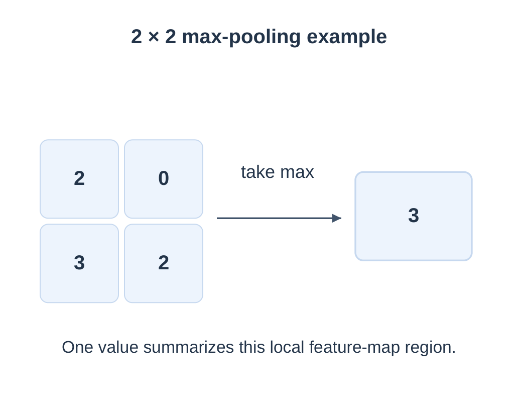
Pooling summarizes a local feature-map region.
Max pooling selects the largest value.
Average pooling takes the mean.
These operations can reduce spatial dimensions and computation.
A basic fixed pooling rule does not learn a weight for every position.
For the feature map:
[[2,0], [3,2]]
A 2 × 2 max-pooling window covering the whole map returns:
max(2,0,3,2) = 3
The corresponding average is:
(2 + 0 + 3 + 2)/4 = 1.75
These are different summaries.

2.21.1 Typical Introductory Pipeline
| Stage | Purpose |
|---|---|
| Prepare image | Use consistent dimensions and value preparation |
| Convolution + activation | Learn and transform local responses |
| Further feature stages | Combine patterns across regions |
| Pooling or another reduction | Summarize spatial information |
| Output head | Produce task-specific predictions |
2.21.2 What CNNs Do and Do Not Guarantee
Local filters can respond to a pattern at several positions, and pooling can reduce sensitivity to some small shifts.
A CNN is not automatically invariant to all translations, rotations, lighting changes or camera types.
Test conditions still matter.
For a classifier, the output head may predict an image category.
A detection system also estimates object locations.
A segmentation system assigns labels to pixels or regions.
CNN features can be used in these different systems. The output requirement determines the rest of the design.
2.21.3 A Short Design Example
To classify fabric images as acceptable or defective:
- Collect examples from relevant materials.
- Prepare images consistently.
- Train an image model.
- Inspect held-out results.
A classifier label alone does not show the exact defect position.
If the practical need is to mark a tear’s location, specify detection or segmentation labels and an evaluation method suited to location quality.
Do not assume that an image-level classifier has solved that additional task.
2.21.4 Historical Context
Yann LeCun and collaborators helped develop influential convolutional approaches for document recognition.
The 1998 work on gradient-based document recognition connects learned filters, network training and practical recognition tasks.
This history illustrates how an architecture can fit the structure of its input.
It does not imply that CNNs are the only possible image architecture or that every computer-vision system uses the same network.
2.22 Computer Vision: How AI Uses Images
Computer vision develops methods for extracting useful information from images or video.
A camera converts light into measurements. Software represents the resulting image as numerical arrays.
A model then transforms those values into a task-specific output.
A grayscale image can be represented by one intensity channel.
A typical color image has red, green and blue channels.
Pixel values are measurements in an encoding, not semantic descriptions such as leaf or disease.

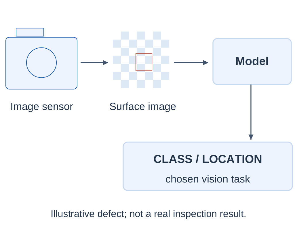
2.22.1 From Pixels to a Prediction
Step 1: Capture a suitable image under known conditions.
Step 2: Prepare its shape and numerical values consistently.
Step 3: Extract or learn relevant visual representations.
Step 4: Generate a category, location or other defined output.
Step 5: Check the result using appropriate reference information.
2.22.2 Main Vision Tasks
| Task | Output | Example |
|---|---|---|
| Classification | Image-level category | Healthy-looking / affected leaf |
| Detection | Object categories and locations | Locate visible surface defects |
| Segmentation | Pixel / region labels | Mark the affected image region |
| Recognition / matching | Similarity or identity decision | Compare a face with enrolled references |
An image model can learn a shortcut.
If every defective sample was photographed on one table and every normal sample on another, the background may be predictive in development but useless for the actual task.
Images of the same object can be highly related.
Split by the underlying object, subject, roll or collection episode when appropriate, rather than allowing near-duplicate frames into both development and test groups.
2.22.3 Sources of Visual Variation
- Lighting, shadows and reflections alter observed values.
- Pose, distance and perspective change appearance.
- Occlusion hides useful regions.
- Different sensors and processing pipelines change inputs.
- Unrepresented materials or conditions can shift the data.
The model processes numerical observations and learns task-related patterns.
A correct label on one image does not establish reliability on every related image.
2.23 Face Recognition and Medical Imaging
2.23.1 Detection Versus Recognition
Face detection locates a face in an image.
Face recognition compares information about a detected face with enrolled references.
Detecting a face does not by itself identify the person.
A recognition pipeline can:
- Detect and align a face.
- Compute a learned representation.
- Compare it with a reference representation.
- Convert a similarity score into a decision using a chosen threshold.
| Task | Question |
|---|---|
| Detection | Is there a face, and where? |
| Verification | Does this face match the claimed identity? |
| Identification | Which enrolled identity, if any, is a match? |
Verification typically compares against a claimed identity.
Identification searches a reference set.
A larger reference set and different operating conditions can change the error situation. A match score is not proof of identity.
Pose, lighting, age differences and occlusion can affect comparisons.
Evaluate relevant populations and conditions. A single overall average can hide important differences.
A strict match threshold can reduce false matches while increasing rejected genuine matches.
2.23.2 Medical-Image Analysis Concepts
AI can support tasks such as identifying image patterns, locating a suspicious region or segmenting an anatomical structure.
Possible inputs include radiographs, scans and microscope images.
The required reference labels and validation depend on the exact task.
A model score is not a confirmed diagnosis.
Image findings must be interpreted with relevant clinical information and qualified review. These examples explain computing concepts and do not provide clinical decision rules.
| Computing Task | Illustrative Output |
|---|---|
| Classification | An image-level flag for review |
| Detection | A proposed region to inspect |
| Segmentation | A boundary around an anatomical area |
| Measurement support | A numerical image-derived measurement |
2.23.3 Why Validation Is Demanding
Different hospitals, devices and collection protocols can produce different image distributions.
Related images from the same patient should not create misleadingly easy development and test comparisons.
A classifier may respond to markings or acquisition artifacts instead of a medically meaningful pattern.
Examine representative external conditions, error types and the limits of reference labels before claiming usefulness.
High accuracy in a constructed classroom dataset is insufficient evidence for deployment.
The underlying distinction between predictions and verified outcomes remains essential.
2.24 Natural Language Processing
Natural Language Processing (NLP) develops computational methods for working with human language.
Tasks include classifying text, extracting information, translating language and producing responses.
The representation must account for meaningful language patterns and context.
Text is converted into computational units such as tokens and numerical representations.
A token is not always a whole word. It may represent a word part, punctuation or another unit chosen by the tokenizer.

2.24.1 Why Context Matters
“The result is good” and “The result is not good” contain many of the same words but express different judgments.
Ignoring negation can reverse a sentiment label.
In “the bank of the river” and “the bank approved a loan,” the same word has different meanings.
A useful representation should use surrounding context rather than assume that each word has one fixed interpretation.
Recognizing the word urgent can support a spam baseline, but it does not provide complete understanding of a message.
Word occurrence, sentence structure and context supply different levels of evidence.
2.24.2 Common NLP Tasks
| Task | Input → Output |
|---|---|
| Text classification | Message → spam / legitimate |
| Sentiment analysis | Review → attitude category or score |
| Information extraction | Sentence → names, dates or relations |
| Translation | Text in one language → another |
| Summarization | Long text → shorter account |
| Question answering | Question + information → answer |
A count-based text classifier may represent a document through word occurrences.
A neural method can learn representations that depend on surrounding units.
Both need evaluation suited to the output. Fluent text does not guarantee factual correctness.
2.24.3 Preparation Decisions
- Choose a tokenizer suited to the language and task.
- Handle missing or malformed text consistently.
- Preserve information such as negation when it matters.
- Separate related documents across evaluation groups carefully.
- Check the languages, spelling styles and domains represented.
Lowercasing and removing punctuation are not universally harmless.
Capitalization can help identify names, and punctuation can affect meaning.
Select transformations for a stated purpose rather than deleting every unusual symbol automatically.
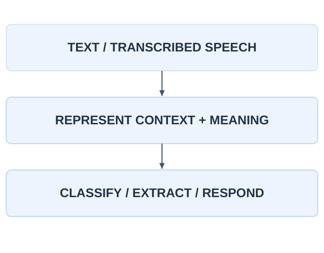
2.25 Speech and Language Processing
Speech begins as an audio signal.
Automatic Speech Recognition (ASR) converts audio into text.
NLP can then interpret the text or perform a language task.
A voice interaction can also use speech synthesis to turn an answer back into audio.
These stages solve different problems.
A word may be transcribed incorrectly because of noise, even if the language component would interpret the correct sentence successfully.
Conversely, a perfect transcript can still be misunderstood.


2.25.1 Trace a Spoken Request
For “show tomorrow’s class schedule”:
Input: A microphone supplies audio.
Recognition: ASR produces a transcript.
Language task: A component identifies the schedule request and relevant date.
Application action: The system retrieves the permitted schedule and formats the response.
Not every stage must be learned, and not every stage is NLP.
Database retrieval and access rules are application functions.
A complete system can combine learned and fixed components.
2.25.2 Challenges in Speech and Text
| Challenge | Possible Consequence |
|---|---|
| Background noise | Words are missed or altered |
| Accent / speaking variation | Training coverage may be insufficient |
| Similar-sounding words | Ambiguous transcription |
| Code-switching | More than one language appears together |
| Context-dependent date | Tomorrow needs a reference date |
| Ambiguous intent | Correct words still allow several requests |
For a classroom demonstration, compare a reference sentence with the transcript and then assess the language task separately.
That separation helps locate an error rather than treating every failure as one unexplained language problem.
2.25.3 Text-to-Speech Is Another Direction
Speech synthesis takes text or a language representation and produces audio.
It is distinct from recognizing incoming speech.
A system may perform both directions during a conversation.
An expressive synthesized voice does not verify the content spoken.
The factual quality of an answer and the audio quality of its delivery are different evaluation questions.
2.25.4 Vision Versus NLP
A camera image is a spatial numerical array.
Text is represented through a sequence of language units.
Both can use learned representations and neural networks, but their structure, errors and outputs differ.
Some tasks combine modalities, such as reading words from an image and then interpreting their meaning.
Optical character recognition supplies recognized text; the subsequent language task operates on that text.
2.26 Engineering Connections
| Stream | Connection to This Unit |
|---|---|
| ECE | Image sensors supply arrays that vision models process |
| BT | Protein sequence can be used for structure prediction |
| AG | Plant images support a defined visual classification task |
| TX | Surface images can support fabric-defect inspection |
For ECE, the sensor is an essential measurement source.
Resolution, exposure, noise and camera placement affect information available to the model.
A poor capture cannot be repaired simply by naming a more complex classifier.
For AG, a leaf-image model can flag a visual category for review.
Different lighting, varieties, growth stages and non-disease damage can make the task difficult.
A photo label is not a complete agronomic assessment.
For TX, classification can flag a patch. Detection or segmentation can help locate a defect.
Sampling across rolls and materials reduces the risk that the model learns only one collection setup.
2.26.1 Other Stream Examples
- CSE can implement and evaluate a classifier.
- EE can study labelled equipment-fault readings.
- CE can explore image-based surface inspection.
- ME can classify condition-monitoring signals.
- CH can predict numerical process-quality values.
Each example needs a precise input, output and validation plan.
Use classification measures for category decisions and MAE for numerical predictions.
A stream abbreviation does not determine the learning method or metric.
2.26.2 BT Connection: AlphaFold
AlphaFold is a prominent protein-structure prediction example.
Its task is to estimate three-dimensional structure from sequence-related information using learned models and other supplied information.
A structure prediction is different from predicting a simple class label.

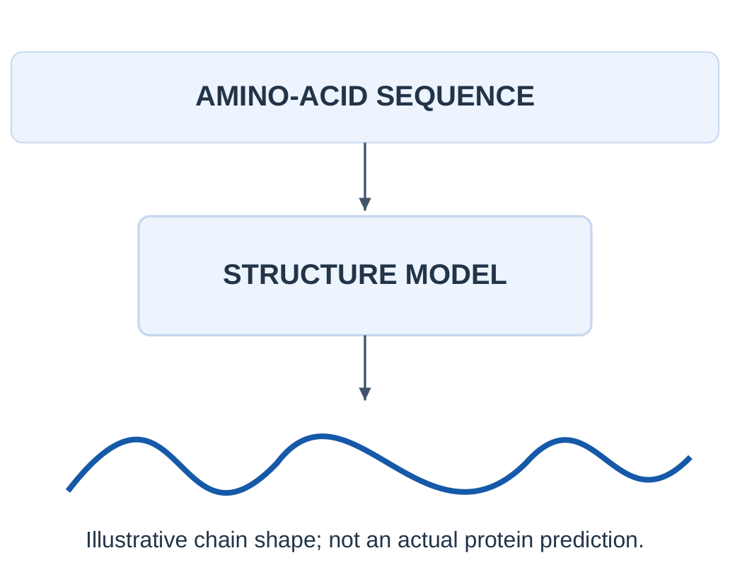
The AlphaFold2 work demonstrated major progress in protein-structure prediction.
Confidence estimates help identify parts that are more or less supported by the model.
A predicted structure should not be treated as equally reliable at every position.
A protein can adopt different conformations and interact with other molecules.
One predicted structure does not explain every motion, biochemical function or experimental condition.
Experimental evidence and domain interpretation remain important.
2.26.3 A Five-Part Application Answer
Step 1: Name the engineering problem precisely.
Step 2: Describe the available input measurements.
Step 3: Specify category, number, region or structure output.
Step 4: Choose a matching evaluation approach.
Step 5: State a concrete data or deployment limitation.
Sensors, labels, representations and evaluation connect mathematical methods to engineering practice.
2.27 Activity: A No-Code Image Classifier
Use Google Teachable Machine for a brief classroom demonstration of image classification.
The supplied syllabus outline suggests an approximately five-minute activity. Actual time depends on preparation, device and training.
The steps below are a plan, not a claim that a model has been trained in these notes.
Choose two nonsensitive object categories, such as a notebook and a pen case.
Use your own permitted objects and images.
The aim is to observe how examples, labels and collection conditions affect a classifier.

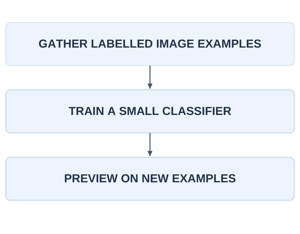
2.27.1 Procedure
Step 1: Open Teachable Machine and choose an image project.
Step 2: Name the two classes clearly.
Step 3: Gather several varied examples per class using permitted images or a camera.
Step 4: Train the project using the available training control.
Step 5: Preview predictions on fresh examples of each class.
Control names and placement can change. Follow the available image-project workflow rather than relying on one screenshot’s exact coordinates.
2.27.2 Make the Check Meaningful
Change object position, distance and background.
If the notebook was always held on the left and the pen case on the right, swap their positions during checking.
This tests whether the classifier used an irrelevant collection pattern.
Do not use nearly identical consecutive frames as your only evidence of generalization.
Record a small independent test with known categories and note the collection conditions.
| Test Case | Actual | Predicted | Observation |
|---|---|---|---|
| New notebook view | Notebook | Record result | Change angle |
| New pen-case view | Pen case | Record result | Change position |
| Same object, new background | Known class | Record result | Check shortcut |
| Unrelated object | Outside classes | Record result | Watch unsupported score |
This is an illustration of evaluation, not a certified product assessment.
2.27.3 Discussion and Submission
- What did the class names represent?
- Which changes caused errors?
- Did a high displayed score always mean a correct label?
- Was the object or the background more influential?
- What would improve the next collection?
Submit the class definitions, example-collection description, test observations and one limitation.
If the interface only offers the trained classes, an unrelated object may still receive one of them.
That does not prove it belongs to either category.
Training examples influence the decision. Varied, relevant collection and a separate check matter more than a polished-looking confidence display.
2.28 Quick Revision: Methods and Measures
| Concept | One-Line Recall |
|---|---|
| KNN | Vote among k nearby labelled examples |
| Naïve Bayes | Prior × conditionally independent likelihood terms |
| K-Means | Assign to centroids and update means |
| Centroid | Mean of assigned numerical points |
| Accuracy | (TP + TN) / total |
| Precision | TP / (TP + FP) |
| Recall | TP / (TP + FN) |
| F1 | 2TP / (2TP + FP + FN) |
| MAE | Average absolute numerical prediction error |
| Neuron | Weighted sum + bias, then activation |
| CNN | Local shared filters create feature maps |
| NLP | Computational processing of human language |
2.28.1 Choose the Method
Nearby labelled reference readings suggest a KNN baseline.
Class priors and simple feature likelihoods suggest Naïve Bayes.
Unlabelled numerical grouping by centroids suggests K-Means.
Learned multilayer image representations suggest a neural architecture such as a CNN.
These are conceptual matches, not automatic recommendations.
A useful design also checks representation, data scale, available labels and the evaluation goal.
2.28.2 Correct These Misconceptions
| Incorrect Idea | Correct Statement |
|---|---|
| KNN k counts classes | It counts selected neighbors |
| K-Means learns known labels | It fits groups without supplied target categories |
| Naïve means all data are independent | The assumption is conditional on class |
| High accuracy finds all rare positives | Recall may still be zero |
| MAE is a classification rate | It measures numerical regression error |
| Every deep model needs a GPU | Small workloads can run on CPUs |
| A classifier locates every defect | Locations require an appropriate output task |
| ASR and NLP are identical | Audio recognition and language tasks differ |
2.28.3 A Connected Case
A team photographs labelled fabric patches and trains a CNN classifier.
The input is an image array, the target is a patch category and the learned filters create intermediate representations.
Held-out patches provide TP, FP, FN and TN for a defined defect-positive class.
If the team instead groups unlabelled texture measurements around centroids, that is a K-Means setup.
If it predicts a numerical defect-area measurement, MAE may become relevant.
The domain stays fabric inspection while the mathematical task changes.
2.29 Examination Practice
2.29.1 Short-Answer Questions
- Define k in KNN and contrast it with k in K-Means.
- State the conditional-independence assumption of Naïve Bayes.
- What is a centroid, and must it be a training point?
- Define TP, FP, FN and TN for a stated positive class.
- Explain why accuracy alone can be misleading.
- Why does MAE use absolute values?
- Identify the roles of weight, bias and activation.
- Distinguish width from depth in a network.
- Why can GPUs accelerate neural-network training?
- Differentiate a CNN filter and a pooling operation.
- Distinguish face detection, verification and identification.
- Explain the relationship between ASR and NLP.
2.29.2 Longer-Answer Questions
- Explain KNN with an ordered-distance example and two limitations.
- Derive Naïve Bayes class comparison from Bayes’ theorem and solve a two-feature example.
- Explain K-Means initialization, assignment, update and stopping with a dry run.
- Compare accuracy, precision, recall and F1 using one confusion matrix.
- Draw a labelled neuron and explain forward computation, loss, gradients and parameter updates.
- Explain CNN filtering and pooling with a numerical example.
- Distinguish image classification, detection and segmentation.
- Explain the stages of a speech-enabled application.
2.29.3 Numerical Practice with Checks
Problem 1: KNN
Training values are 1(A), 2(A), 4(B), 6(B) and 8(B).
Query = 3.2.
Uniform k = 3.
Find the nearest labels and predicted class.
Check: B, A, A; predict A.
Problem 2: K-Means
Values are {1,2,4,8,9,10}.
Initial centroids are 1 and 4.
Show two assignments and updates.
Check: First means are 1.5 and 7.75. Stable means are 7/3 and 9.
Problem 3: Classification Metrics
TP = 18, FP = 6, FN = 12, TN = 24.
Calculate accuracy, precision, recall and F1.
Check:
Accuracy = (18 + 24)/60 = 0.70
Precision = 18/24 = 0.75
Recall = 18/30 = 0.60
F1 = 36/(36 + 6 + 12) = 2/3
Problem 4: MAE
Actual values = {5,10,15}
Predicted values = {6,8,18}
Check:
Absolute errors = {1,2,3}
MAE = (1 + 2 + 3)/3 = 2 target units
Problem 5: Neuron
x1 = 2, x2 = 1, w1 = 0.5, w2 = −1, b = 0.2
Use ReLU activation.
Check: Weighted input = 0.2; output = 0.2.
Problem 6: CNN
Apply filter [[1,0],[0,1]] to input [[1,0,2],[2,1,0],[0,1,1]].
Use stride one, no padding and no filter flipping.
Check: Feature map = [[2,0],[3,2]].
Whole-map max pooling gives 3.
2.29.4 Diagram Practice
Draw:
- KNN vote workflow
- K-Means assignment-and-update loop
- Labelled confusion matrix
- Artificial neuron
- Input, hidden and output layers
- CNN patch calculation
- Pooling operation
- Audio-to-language pipeline
Name what every arrow carries: examples, feature values, scores, gradients or text.
A longer answer should include a definition, labelled figure or table, traceable example and one meaningful limitation.
Explain what the computed result establishes rather than ending at a number.
COMPLETE EXPLANATIONS FOR EXAM ANSWERS
The following connected answers support revision from these AI and Prompt Engineering Unit 2 Notes.
Explain KNN with a Numerical Example
K-Nearest Neighbors classification predicts a query’s label from nearby labelled reference examples.
Define the input representation and distance, calculate the distances, select the k nearest examples and apply the stated voting rule. The parameter k counts neighbors, not classes.
For values 1(A), 2(A), 4(B), 6(B) and 8(B), a query at 3.2 has distances 2.2, 1.2, 0.8, 2.8 and 4.8.
The three closest examples are 4(B), 2(A) and 1(A). A uniform k = 3 vote therefore predicts A. With k = 1, the prediction would instead be B.
Distance depends on representation and scale. An irrelevant high-range feature can distort the neighborhood.
Choose preparation and k using suitable development evidence, state a tie policy and check relevant unseen examples.
A unanimous vote does not guarantee that a query far outside the reference distribution is well supported.
Derive the Naïve Bayes Class Comparison
Bayes’ theorem gives:
P(C | X) = P(X | C)P(C)/P(X)
For a fixed query X, the evidence P(X) is common to candidate classes.
Provided the comparison is defined, the class maximizing the posterior also maximizes the numerator.
Naïve Bayes assumes features are conditionally independent given the class.
It approximates the joint likelihood as a product of feature likelihoods:
Score(C) = P(C) × product of P(xj | C)
This is not a claim that all features are unconditionally independent.
In the message example, Spam has prior 0.4 and present-feature likelihoods 3/4 and 3/4, giving score 0.225.
Legitimate has prior 0.6 and likelihoods 1/6 and 2/6, giving approximately 0.03333.
Spam wins.
Dividing by the sum of these two fitted scores gives normalized values 27/31 and 4/31. It does not establish a real-world success rate.
Laplace smoothing can address zero-frequency estimates. For a binary feature it uses:
(count + 1)/(class count + 2)
It does not repair incorrect labels, feature dependence or distribution change.
Explain K-Means with Assignment and Update
K-Means groups unlabelled numerical points around k centroids.
Choose initial centers, assign every point to a nearest center, replace each center by the mean of its assigned points and repeat until a specified stopping condition holds.
The standard objective is the within-cluster sum of squared distances.
For {1,2,4,8,9,10}, initialize the centers at 1 and 4.
The first assignment gives {1,2} and {4,8,9,10}, whose means are 1.5 and 7.75.
Reassignment moves 4 into the first cluster.
The new groups are {1,2,4} and {8,9,10}, with means 7/3 and 9.
The midpoint between the final means is 17/3. Each point remains on the appropriate side, so the groups are stable.
The final squared-error objective is:
14/3 + 2 = 20/3
A centroid need not be an observed point, and a cluster number is not a verified semantic class.
Initialization, scaling, outliers and the chosen k affect the result.
Compare Accuracy, Precision, Recall, F1 and MAE
First define the positive class.
TP and TN are correct positive and negative predictions.
FP is a negative case incorrectly flagged positive.
FN is a positive case incorrectly missed.
For TP = 30, FP = 10, FN = 20 and TN = 40, there are 100 cases.
Accuracy is:
70/100 = 0.70
Precision is:
30/40 = 0.75
It asks how many positive predictions were correct.
Recall is:
30/50 = 0.60
It asks how many actual positives were found.
F1 is:
60/(60 + 10 + 20) = 2/3
It is the harmonic balance of precision and recall, not their arithmetic mean.
High accuracy can conceal failure on a rare class. Predicting negative for all 95 negatives and 5 positives gives 95% accuracy but zero recall.
Undefined denominators require an explicit reporting convention.
MAE instead evaluates numerical predictions. Average the absolute prediction errors and retain target units.
For absolute errors 2,2,3,3:
MAE = 2.5 target units
Applying MAE to arbitrary unordered category codes does not give a meaningful classification measure.
Explain a Neural-Network Training Cycle
A neuron computes:
z = sum(wj xj) + b
It then applies:
a = f(z)
Layers pass their outputs onward.
A forward pass produces a prediction; a loss compares that output with the target under a chosen objective.
Backpropagation computes gradients of the loss with respect to parameters.
An optimizer then uses those gradients to update weights and biases.
In simple gradient descent:
w_new = w − learning rate × gradient
With w = 0.50, learning rate 0.10 and gradient 0.20:
w_new = 0.48
Repeat over batches and epochs while monitoring suitable validation evidence.
Falling training loss alone does not establish improving generalization.
An independent final test checks the selected process.
Ordinary inference uses fitted parameters and does not necessarily update them.
Explain CNN Filtering and Pooling
A CNN applies learned local filters at multiple spatial positions.
Reusing the same filter weights is weight sharing.
For input [[1,0,2],[2,1,0],[0,1,1]] and filter [[1,0],[0,1]], stride one and no padding, the unflipped multiply-and-add operation produces:
[[2,0], [3,2]]
The upper-left value is:
1×1 + 0×0 + 2×0 + 1×1 = 2
Repeat at the remaining valid positions to complete the feature map.
This is the cross-correlation convention commonly called convolution in CNNs.
A 2 × 2 max-pooling operation over the whole feature map returns 3.
Average pooling returns 1.75.
The pooling rule summarizes a region separately from learning the filter.
The output task still matters: an image classifier returns a category, while detection and segmentation require location-related outputs and suitable reference labels.
FORMULA SHEET WITH CONDITIONS AND CHECKS
| Relation | Condition / Meaning |
|---|---|
| d(x,q) = sqrt(sum of (xj − qj)²) | Euclidean distance on meaningfully represented numerical features |
| KNN prediction = majority label among selected k neighbors | Uniform voting; define distance and tie handling |
| P(C | X) = P(X | C)P(C)/P(X) | Bayes’ theorem where P(X) is positive |
| Naïve Bayes score = P(C) × product of P(xj | C) | Conditional-independence approximation given the class |
| Binary Laplace estimate = (count + 1)/(class count + 2) | Binary feature with both values smoothed consistently |
| Centroid = mean of assigned points | Compute each coordinate separately; empty groups need a policy |
| K-Means objective = sum of squared point-to-assigned-centroid distances | Standard Euclidean K-Means objective |
| Accuracy = (TP + TN)/(TP + TN + FP + FN) | Fraction of all predictions correct |
| Precision = TP/(TP + FP) | Correct fraction among predicted positives |
| Recall = TP/(TP + FN) | Found fraction among actual positives |
| F1 = 2PR/(P + R) = 2TP/(2TP + FP + FN) | Harmonic balance; state zero-denominator conventions |
| MAE = sum of absolute prediction errors / n | Numerical regression; retains target units |
| z = sum(wj xj) + b; a = f(z) | Neuron weighted input and activated output |
| ReLU(z) = max(0,z) | Zero for negative inputs; unchanged nonnegative inputs |
| Sigmoid(z) = 1/(1 + exp(−z)) | Maps finite real inputs between zero and one |
| Dense-layer parameters = inputs × neurons + neurons | One bias per neuron in the specified fully connected layer |
| w_new = w − learning rate × gradient | Simple gradient-descent update |
| Output size = floor((N + 2P − F)/S) + 1 | One spatial dimension; valid stride, padding and filter settings |
| Max pooling = maximum in the selected region | Average pooling instead takes the region’s mean |
Memory check: Neighbors vote, Bayes compares probability scores, K-Means updates means, metrics count defined outcomes, neurons transform weighted inputs and CNN filters share local weights.
QUICK REVISION: EXPLAIN AND CONNECT
What Does k Mean in KNN and K-Means?
In KNN it counts selected neighbors.
In K-Means it counts fitted clusters or centroids.
Neither meaning automatically equals the number of true real-world categories.
Must a Centroid Be a Training Point?
No. It is an arithmetic mean and can lie between observed points.
What Does the Naïve Bayes Assumption Say?
Features are conditionally independent given the class.
It does not say that all recorded variables are unrelated in the full population.
Why Can Accuracy Mislead?
A large majority class can dominate the correct-count fraction while the model misses every rare positive.
Inspect the confusion matrix and relevant error types.
How Do Precision and Recall Differ?
Precision uses predicted positives as its denominator.
Recall uses actual positives.
Write the group being counted before substituting numbers.
Is MAE a Classification Percentage?
No. It measures average absolute error for numerical predictions and keeps the target’s units.
Does More Training Always Improve a Model?
No. Training-specific fitting can improve training loss while worsening held-out performance.
Monitor relevant validation evidence.
Does Backpropagation Perform the Entire Update?
Backpropagation computes gradients.
The optimizer uses them to update parameters under a specified rule.
Does Every Deep Model Need a GPU?
No. A GPU can accelerate suitable parallel workloads, but small models can run on a CPU.
Hardware does not repair poor labels or leakage.
Are Convolution and Pooling the Same?
No. A convolutional layer applies shared local filter weights.
A pooling rule summarizes a region, such as by taking its maximum.
Does Classification Locate a Defect?
An image-level category does not give the defect’s position.
Detection or segmentation requires a suitable location-related output and evaluation.
Are ASR and NLP Identical?
No. ASR turns audio into text.
NLP performs language tasks on text or related language representations.
Their errors should be checked separately.
Use these AI and Prompt Engineering Unit 2 Notes to revise definitions alongside numerical traces and diagrams. Additional resources are available at www.notesgallery.com. The university website is https://aktu.ac.in.