
University: Dr. A.P.J. Abdul Kalam Technical University (AKTU)
Programme: B.Tech First Year, Semester I & II
Course Codes: AME101A / AME201A
Branches: Common to All
Unit: III — Machine Elements and Power Transmission
Introduction
Machine Elements and Power Transmission explains how individual components join parts, support rotation and deliver useful motion. The applications connect these elements to robotic joints, 3D-printer axes and drone motors.
A working machine contains several different mechanical functions. A motor supplies torque and speed. A transmission changes or transfers motion. Shafts and hub connections carry useful torque. Bearings support rotating members, while housings and frames receive reaction loads.
Understanding the assembly requires more than identifying component names. The torque path and support path must be traced separately. A bearing can support a shaft without acting as the intentional connection that transmits torque from the shaft to a pulley. A key can transmit torque without automatically retaining the pulley axially.
The numerical relationships in this unit describe supplied geometrical, static and steady-motion models. A speed ratio predicts nominal motion. A force divided by an area gives a stated average intensity. Neither result automatically establishes fatigue life, complete positioning accuracy or the capacity of every part in an assembly.
Topic Map
| Topic | Main Coverage |
|---|---|
| Threaded fasteners | Bolts, nuts, washers, screws and mating threads |
| Thread geometry | Major diameter, minor diameter, pitch and lead |
| Joint behaviour | Grip, engagement, clamping and retention |
| Shaft connections | Keys, keyways, hubs and separate axial retention |
| Rotating members | Shafts, axles, torque, speed and power |
| Couplings | Rigid and flexible types, alignment and limits |
| Bearings | Rings, rolling elements, cages, radial and axial loads |
| Belt drives | Friction belts, timing belts and pulley motion |
| Printer motion | Travel per revolution and commanded increments |
| Chain drives | Pitch, sprockets, mean speed and ratios |
| Gear trains | External meshes, idlers and compound reductions |
| Applications | Robotic joints and drone-motor bearings |
Symbols and Conventions
| Symbol | Meaning |
|---|---|
| N | Rotational speed in rpm |
| ω | Angular speed in rad/s |
| T | Torque, normally in N·m |
| P | Mechanical power in W |
| η | Efficiency of the stated transmission |
| F | Force in N |
| σ | Average normal stress |
| τ | Average shear stress |
| A | Resisting area |
| p | Compatible thread, belt or chain pitch |
| l | Screw lead |
| z | Tooth count |
| D, d | Stated diameters |
| r | Stated effective radius |
| Fr | Radial force |
| Fa | Axial force |
Reduction is defined here as:
Reduction = Input speed / Output speed
Torque calculations must use consistent units. A torque in N·m must be converted to N·mm when a diameter or radius is inserted in millimetres.
Rotation directions must use one common viewing side. Looking at opposite ends of the same shaft reverses the apparent clockwise or anticlockwise description.
How to Study This Unit
- Identify the component and its principal function.
- Trace torque and support loads separately.
- Distinguish pitch from lead.
- Identify the actual mating thread.
- Check grip, usable engagement and clearance references.
- Use the stated resisting area.
- Define driver and driven members before calculating a ratio.
- Convert rpm before using P = Tω.
- Apply efficiency at the boundary for which it is supplied.
- Separate nominal command spacing from actual accuracy.
- State the assumptions behind equal load sharing.
- Interpret a screening result only within its supplied criteria.
1. Machine Elements and the Power Path
A machine element performs a useful mechanical function within an assembly.
Fasteners join parts. Shafts carry torque. Couplings connect shafts. Bearings support relative motion. Belts, chains and gears transmit motion between members.
The same element can appear in a robot, printer, motor or cooling assembly.

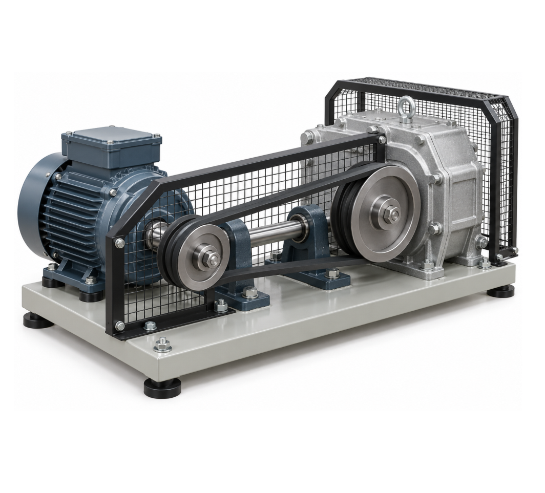

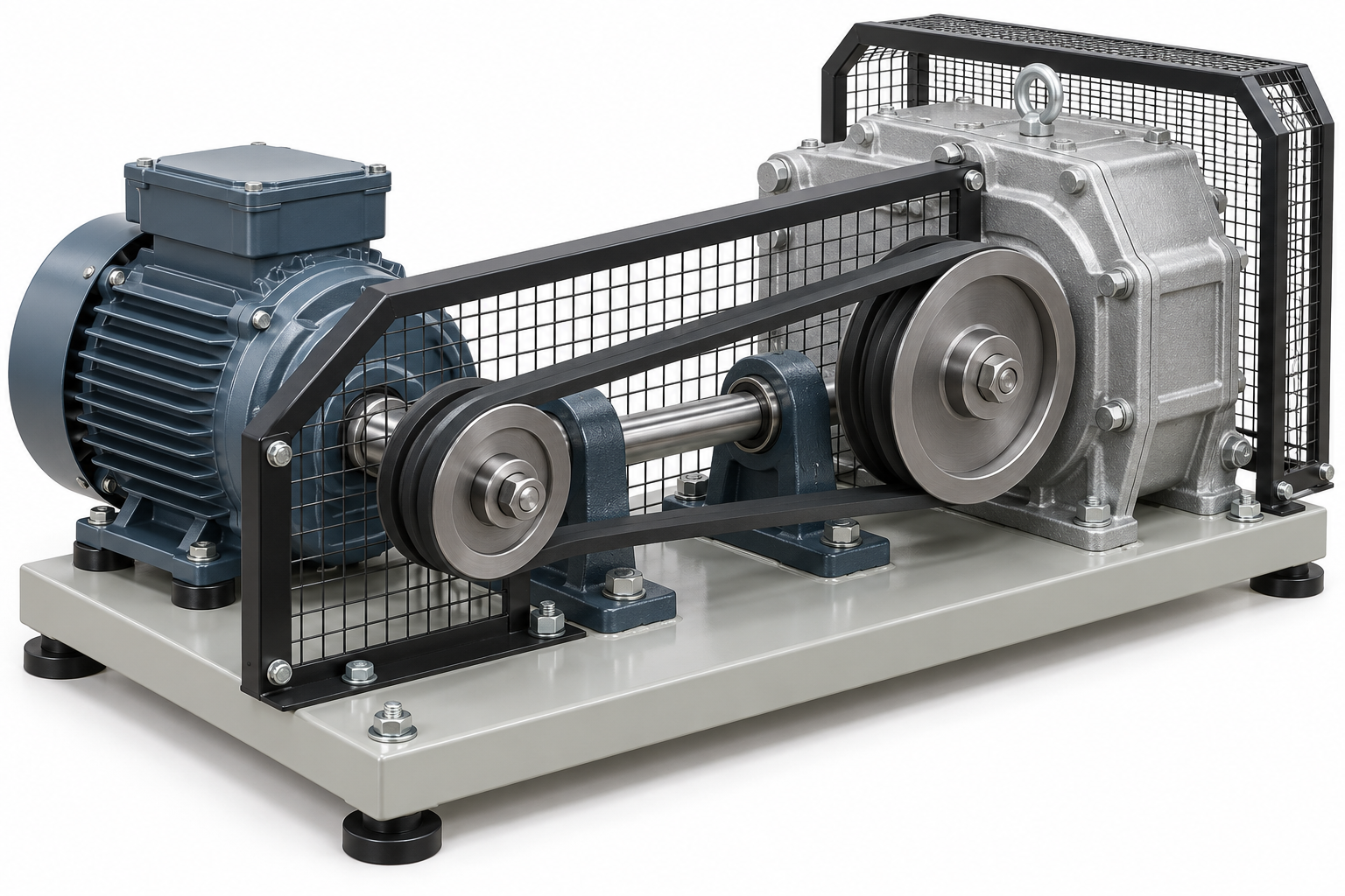

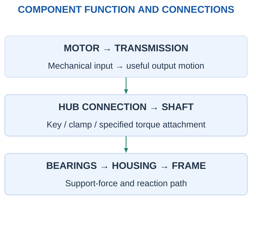
A power path follows energy from the source to the load.
A support path follows forces into bearings, housings and the frame.
The paths are related, but they are not identical. A rolling bearing supports the shaft and allows intended rotation. It normally does not replace the key, clamp or other deliberate connection between that shaft and its gear or pulley.
Three Questions About a Component
- What motion or load does it transmit or constrain?
- Which neighbouring parts connect to it?
- What operating conditions affect its suitability?
A useful application answer identifies an element and explains its mechanical job. Listing bolts, bearings and gears without showing their connections does not explain the assembly.
Power and Loss
For a supplied transmission efficiency:
Pout = ηPin
The represented loss rate is:
Ploss = Pin − Pout
For constant operation over time t:
Eout = Pout t
The supporting reactions cannot be determined from a power balance alone. Their calculation also needs geometry and load information.
Worked Problem 3.1: Power Through a Transmission
Problem: A motor supplies 200 W mechanical power to a transmission with efficiency 0.9. It operates steadily for 30 s. Find output power, loss rate and output energy.
Step 1: Output power is 0.9 × 200 = 180 W.
Step 2: Loss rate is 200 − 180 = 20 W.
Step 3: Output energy is 180 × 30 = 5400 J.
Step 4: Input energy is 6000 J. Represented loss energy is 600 J, so 6000 = 5400 + 600 J.
The loss leaves the useful mechanical power path. It is not additional output.
Worked Problem 3.2: A Larger Transmission Input
Problem: Input is 500 W, efficiency is 0.8 and operating time is 60 s.
Step 1: Pout = 0.8 × 500 = 400 W.
Step 2: Ploss = 500 − 400 = 100 W.
Step 3: Eout = 400 × 60 = 24000 J.
Step 4: Input energy is 30000 J and loss energy is 6000 J.
The power balance does not establish the force on an individual bearing or fastener. Those quantities belong to a separate support-load model.
2. Bolts, Nuts, Washers and Detachable Joints
Threaded fasteners allow parts to be assembled and, in suitable arrangements, separated again.
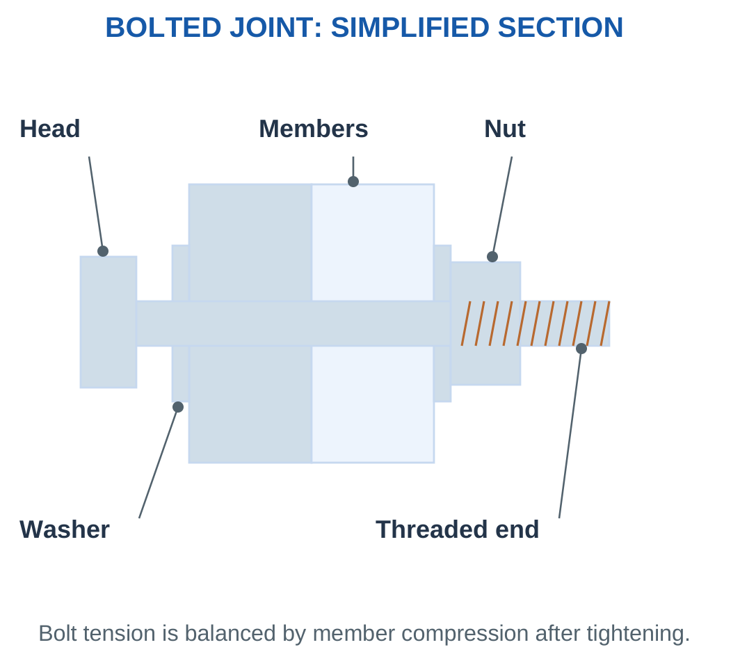
A common bolted joint has a bolt passing through clearance holes and engaging a separate nut. The head and nut bear against the joined members, often through washers.
Tightening develops axial tension in the bolt and compression in the clamped stack.

Main Parts
| Part | Introductory Role |
|---|---|
| Bolt head | Reaction surface and driving feature |
| Shank | Extends through the grip region |
| External thread | Engages the mating internal thread |
| Nut | Provides a separate mating thread |
| Washer | Bearing, spacing or specified retention function |
| Joined members | Carry clamping compression |
A washer can spread local bearing contact, protect a surface, provide spacing or perform a particular locking function according to its design.
An ordinary flat washer is not automatically a positive anti-loosening device.
Tightening Torque and Bolt Tension
Tightening torque is a turning effect.
Bolt tension is an axial force.
They have different units, and their relationship depends strongly on thread and bearing-surface friction.
A desired clamp force cannot be converted into a real installation torque without the appropriate supplied model or assembly information.
Clearance and Mating Threads
A clearance hole allows the bolt to pass through. It is not the same as a tapped hole.
The actual mating arrangement determines where the internal thread lies and how the fastener is retained.
A geometrically long enough bolt may still have unsuitable thread start, runout or usable engagement.
Worked Problem 3.3: Bolt-and-Nut Length Budget
Problem: Two plates are 8 and 10 mm thick. Two washers are 1.5 mm each. Under-head bolt length is 30 mm, and the nut occupies 6 mm after the stack.
Step 1: Plate thickness is 8 + 10 = 18 mm.
Step 2: Washer allowance is 2 × 1.5 = 3 mm. Occupied grip is 21 mm.
Step 3: Projection beyond the nut is 30 − 21 − 6 = 3 mm.
Step 4: This checks the supplied length budget only. Actual engagement, runout and approved assembly requirements still need consideration.
Worked Problem 3.4: Another Bolt Stack
Problem: Plates are 6 and 12 mm, two washers are 2 mm each, under-head length is 35 mm and nut axial length is 8 mm.
Step 1: Plate stack is 18 mm.
Step 2: Washers add 4 mm, giving 22 mm occupied grip.
Step 3: Projection is 35 − 22 − 8 = 5 mm.
Step 4: Positive projection alone does not establish adequate thread engagement, strength or clamp force.
The geometry must be interpreted using the defined reference from beneath the bolt head.
3. Screws and Their Common Uses
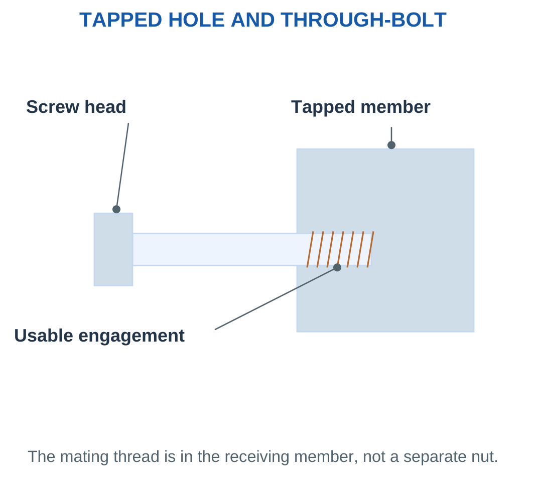
A screw commonly engages a tapped hole or forms a mating thread in a suitable receiving material.
A bolt-and-nut arrangement and a screw-in-tapped-hole arrangement provide useful teaching distinctions. Actual naming can depend on the standard and product.
The engagement should therefore be identified from the assembly rather than appearance alone.

Common Screw Functions
Machine screws use specified machine threads in a suitable nut or tapped hole.
Cap screws provide a headed fastening arrangement, often with an internal driving feature.
Set screws can locate or secure a hub relative to a shaft in an appropriate design.
Self-tapping screws create or form a mating thread in a suitable prepared receiving material.
These arrangements are not universally interchangeable.
A self-tapping fastener is not automatically a suitable substitute in a repeatedly assembled precision joint. A set screw does not automatically transmit any requested torque without slip or local damage.
Blind-Hole Bottoming
A screw can bottom in a blind hole before producing the intended clamp.
It can feel tight while failing to compress the parts correctly.
The usable entry length, usable tapped depth and bottom clearance must therefore be distinguished.
The available depth may exclude incomplete threads or a drill-point region in the stated model.
Worked Problem 3.5: Blind-Hole Clearance
Problem: Usable under-head length is 18 mm, clamped stack is 6 mm and usable blind tapped depth is 15 mm. Required bottom clearance is at least 2 mm.
Step 1: Entry into the receiving member is 18 − 6 = 12 mm.
Step 2: Remaining bottom space is 15 − 12 = 3 mm.
Step 3: The 2 mm requirement passes. Maximum usable under-head length by this criterion is 6 + 15 − 2 = 19 mm.
Step 4: Minimum engagement, thread stripping, screw strength and clamp force remain separate requirements.
Worked Problem 3.6: Deeper Receiving Member
Problem: Under-head length is 20 mm, stack is 8 mm, usable depth is 16 mm and required bottom clearance is 2 mm.
Step 1: Entry is 20 − 8 = 12 mm.
Step 2: Remaining bottom space is 16 − 12 = 4 mm.
Step 3: The clearance criterion passes. Maximum length from this one check is 8 + 16 − 2 = 22 mm.
Step 4: A screw can satisfy bottom clearance and still fail another engagement or strength condition.
4. Thread Geometry and Designation
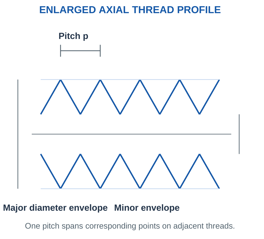
A screw thread is a helical ridge around a cylindrical or conical surface.
The major diameter is the largest thread diameter.
The minor diameter is the smallest.
The pitch diameter is a functional reference associated with thread geometry and fit.
Pitch p is the axial distance between corresponding points on adjacent threads.

Metric Designation
For a designation such as:
M6 × 1
- M identifies the metric thread family.
- 6 is nominal major diameter in millimetres.
- 1 is pitch in millimetres.
This does not specify every fit, material, strength class, finish or product detail.
At the same nominal diameter, a smaller single-start pitch gives more turns for the same axial advance.
A finer thread is not universally better for every material and service.
Thread Stress Area
The nominal major-diameter circle is not automatically the tensile stress area of a threaded fastener.
If a problem supplies tensile stress area, use it.
Pitch is a distance. It should not be confused with a revolution count or rotational speed.
Worked Problem 3.7: Pitch from Eleven Crests
Problem: Eleven consecutive corresponding crests span 10 mm from first to last. Nominal metric diameter is 6 mm.
Step 1: Eleven crests define 10 intervals.
Step 2: p = 10/10 = 1 mm.
Step 3: The diameter-pitch portion is M6 × 1.
Step 4: Pitch equals lead only for a single-start thread. Crest-spacing measurement alone does not identify the number of starts.
Thread Pitch Inspection

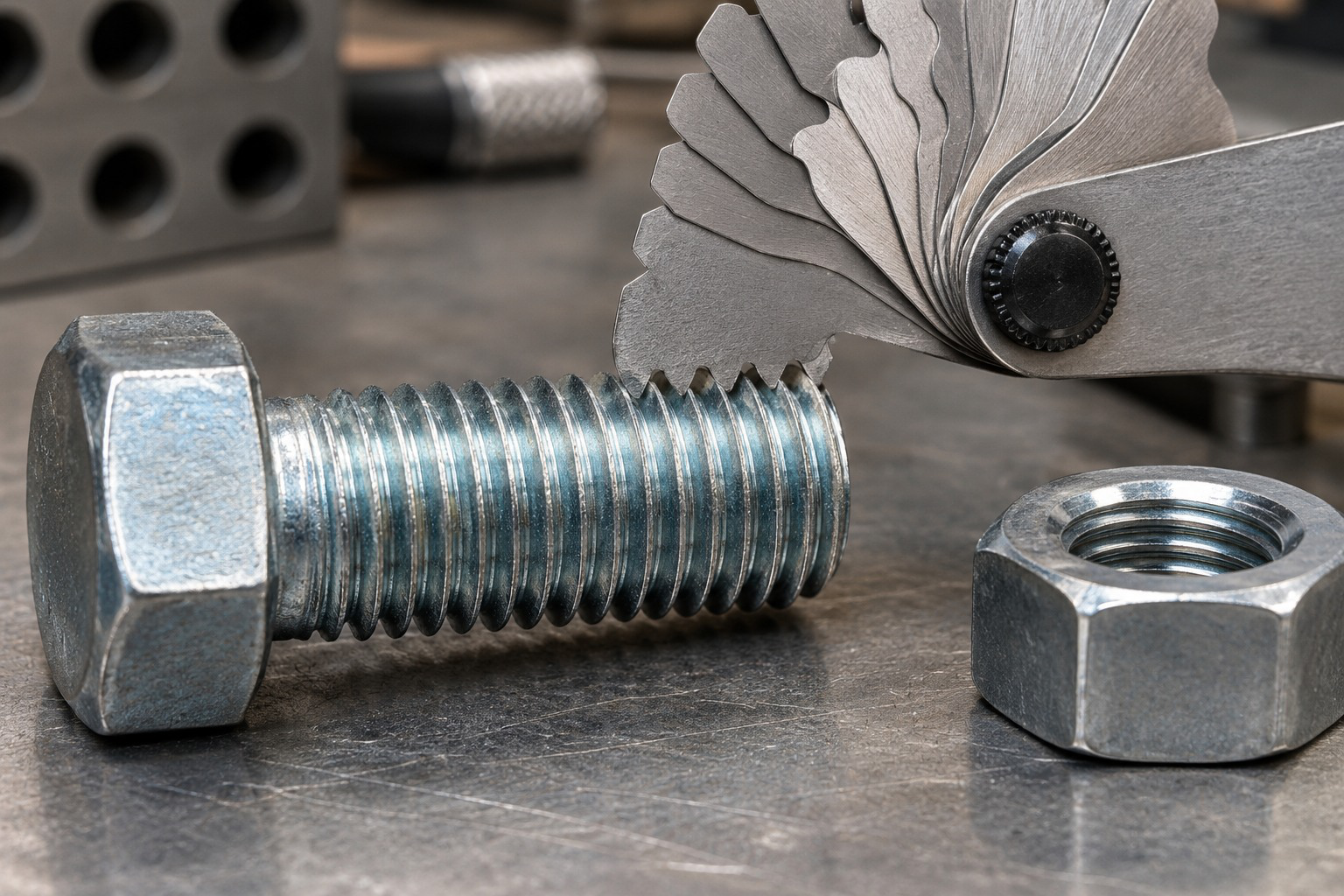
Counting crests and counting intervals are different operations.
The measured span must be divided by the number of pitch intervals between the selected corresponding features.
Worked Problem 3.8: Pitch from Five Crests
Problem: Five corresponding crests span 8 mm. Supplied nominal diameter is 12 mm.
Step 1: There are 5 − 1 = 4 intervals.
Step 2: p = 8/4 = 2 mm.
Step 3: The diameter-pitch portion is M12 × 2.
Step 4: This is not a complete procurement specification and does not by itself reveal lead for a multi-start thread.
5. Pitch, Lead and Screw Travel
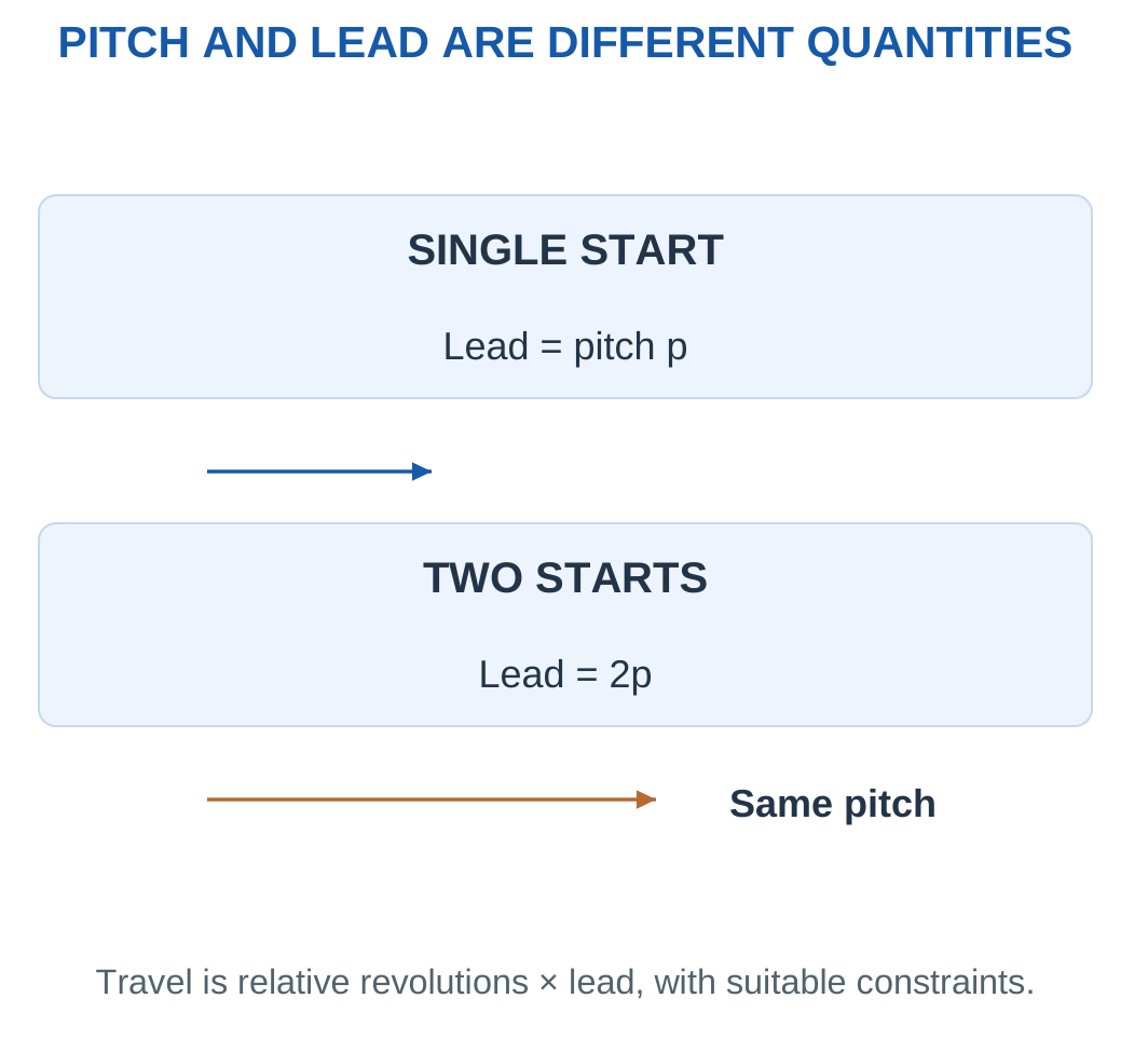
Lead is the axial advance per full relative revolution in the specified motion arrangement.
For a single-start thread:
Lead = Pitch
For s starts:
Lead = s × Pitch
The starts are separate interleaved helices.

Ideal travel is:
x = Number of revolutions × Lead
If the screw is axially fixed and the nut is prevented from rotating:
v = N × Lead / 60
With lead in mm/rev and N in rpm, speed is in mm/s.
Motion Constraints and Direction
The screw and nut require suitable constraints for rotation to produce the intended translation.
Handedness determines advance direction for the stated rotation and viewpoint.
Clockwise and anticlockwise descriptions should identify the viewing end.
Nominal Travel and Accuracy
The geometric equation omits backlash, elastic deformation, lost steps, control error and travel limits.
A fastening screw is not automatically a precision motion screw.
A timing-belt axis uses pulley tooth count and pitch instead of screw lead.
Lead-Screw Linear Axis

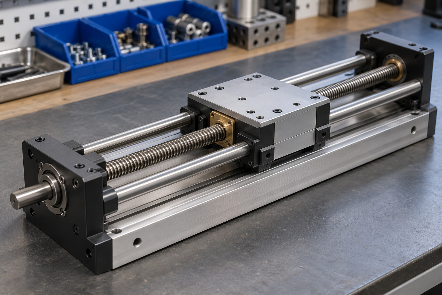
Nominal travel, command counts and measured positioning accuracy are separate quantities.
Worked Problem 3.9: Two-Start Screw
Problem: Pitch is 2 mm with two starts. An axially fixed screw turns eight revolutions at 90 rpm while the nut cannot rotate.
Step 1: Lead = 2 × 2 = 4 mm/rev.
Step 2: Travel = 8 × 4 = 32 mm.
Step 3: v = 90 × 4/60 = 6 mm/s.
Step 4: Time is 8/(90/60) = 5.33333 s.
Speed multiplied by time recovers 32 mm.
Worked Problem 3.10: Three-Start Screw
Problem: Pitch is 1.5 mm, there are three starts and the screw makes ten revolutions at 60 rpm.
Step 1: Lead = 3 × 1.5 = 4.5 mm/rev.
Step 2: Travel = 10 × 4.5 = 45 mm.
Step 3: v = 60 × 4.5/60 = 4.5 mm/s.
Step 4: Time is 10 s, and 4.5 × 10 = 45 mm.
The pitch is 1.5 mm, but using that as travel per turn would underpredict motion by a factor of three.
6. Clamping, Grip and Thread Engagement
Preload is the initial fastener tension developed through tightening.
Before external separating load is applied, this tension is balanced by compression in the clamped members.
Maintained clamping can help resist separation and relative movement, but the required value depends on the complete joint.

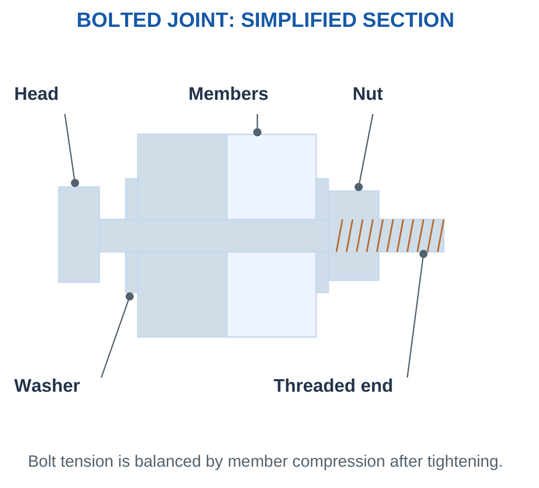
Grip and Engagement
Grip length describes the clamped stack through which the fastener passes.
Thread engagement is the effective axial mating length of external and internal threads.
A bolt can have substantial grip but inadequate nut engagement.
A screw can have sufficient overall length yet bottom before clamping.
A stack calculation therefore checks geometry, not every functional requirement.
External Separating Load
In a preloaded joint, external load can reduce member compression and increase bolt force according to stiffness and load path.
The full external load should not automatically be added to initial preload unless the supplied model explicitly states that relationship.
Worked Problem 3.11: Retained Clamp after Settling
Problem: Initial measured clamp is 4000 N. Supplied reduction is 500 N. Required retained clamp is at least 3000 N.
Step 1: Retained clamp = 4000 − 500 = 3500 N.
Step 2: Reduction = 500/4000 × 100 = 12.5%.
Step 3: 3500 N ≥ 3000 N, so the stated criterion passes.
Step 4: The arithmetic does not identify the cause or prescribe a revised tightening torque.
Worked Problem 3.12: Retained Clamp Below Requirement
Problem: Initial clamp is 6000 N, reduction is 1800 N and requirement is 4500 N.
Step 1: Retained clamp = 4200 N.
Step 2: Reduction = 1800/6000 × 100 = 30%.
Step 3: 4200 N < 4500 N, so the supplied criterion fails.
Step 4: Joint stiffness, settling, service and measurement information are needed before deciding the physical remedy.
Worked Problem 3.13: Another Clamp Check
Problem: Initial clamp is 3000 N, reduction is 600 N and requirement is 2000 N.
Step 1: Retained clamp = 2400 N.
Step 2: Reduction = 20%.
Step 3: The retained force exceeds the 2000 N requirement.
Step 4: Passing this criterion does not establish every fastener or member limit.
7. Introductory Fastener Force and Area Checks
For a supplied central direct-load model:
σavg = F/A
With force in N and area in mm²:
1 N/mm² = 1 MPa
If n identical fasteners explicitly share a central load equally:
Ffastener = Ftotal/n

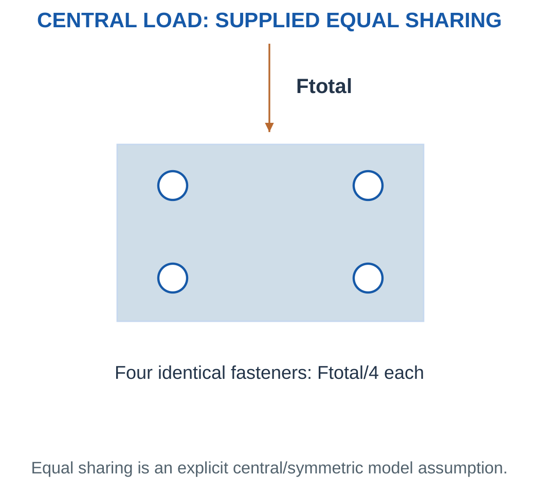
A threaded fastener in tension uses its supplied tensile stress area.
An explicitly smooth-shank shear model uses the specified shear section and plane.
Other possible limits include stripping, bearing contact, member failure, eccentric loading, fatigue and loss of clamp.
Why Equal Sharing Needs Justification
An eccentric bracket can load fasteners unequally.
Dividing total force by count without considering geometry can understate the most heavily loaded fastener.
After calculating stress, multiply it by area to recover force as a dimensional check.
Worked Problem 3.14: Four Fasteners in Tension
Problem: A central 12000 N load is equally shared by four fasteners. Each tensile stress area is 20 mm². Allowable average stress is 180 MPa.
Step 1: Ffastener = 12000/4 = 3000 N.
Step 2: σ = 3000/20 = 150 MPa.
Step 3: 150 ≤ 180 MPa, so the supplied criterion passes.
Step 4: Four times the per-fastener force recovers 12000 N.
The supplied tensile stress area must not be replaced with the nominal diameter circle.
Worked Problem 3.15: Six Fasteners
Problem: A central 18000 N load is shared equally by six fasteners. Area is 30 mm² each and allowable stress is 120 MPa.
Step 1: Ffastener = 3000 N.
Step 2: σ = 3000/30 = 100 MPa.
Step 3: The 120 MPa criterion passes.
Step 4: The result is an average tension check under explicit equal sharing, not a complete joint rating.
Worked Problem 3.16: A Failed Stress Criterion
Problem: An 8000 N load is shared by four fasteners, each with area 14 mm² and allowable stress 130 MPa.
Step 1: Ffastener = 2000 N.
Step 2: σ = 2000/14 = 142.857 MPa.
Step 3: 142.857 > 130 MPa, so the criterion fails.
Step 4: The force check is 4 × 2000 = 8000 N.
A different resisting area or load distribution would require a different calculation.
8. Retention, Loosening and Practical Inspection
A threaded joint must maintain its intended function throughout service.
Vibration, settling, temperature change and inadequate clamping can contribute to loosening or reduced effectiveness.
Different retention methods operate through different mechanisms and are not interchangeable in every application.

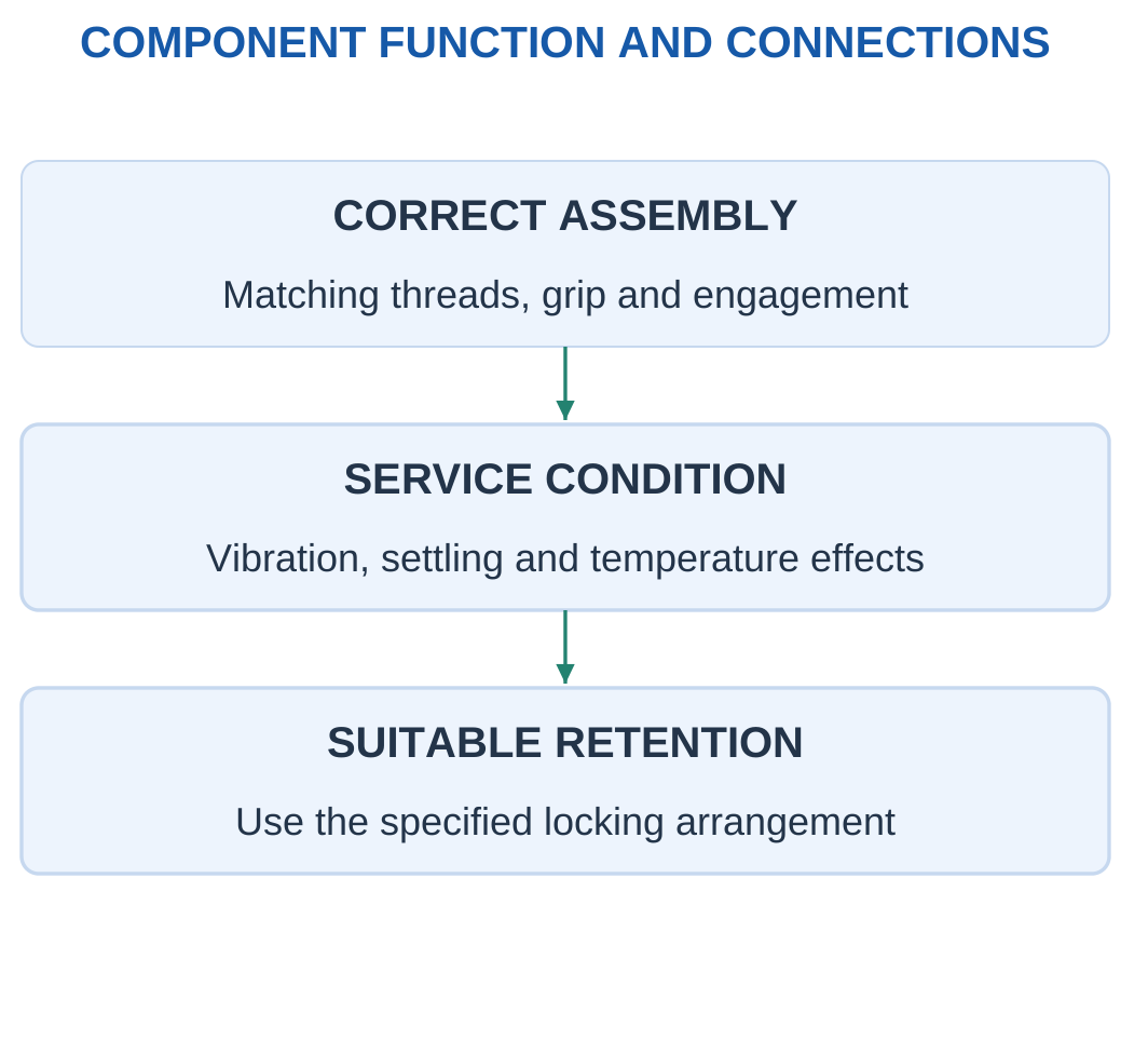
Examples include suitable prevailing-torque nuts, specified thread-locking compounds, mechanical locking arrangements and designed locking hardware.
A castellated nut and correctly arranged split pin provide a physical retention feature in an appropriate assembly.
An ordinary flat washer alone is not proof against self-loosening.
Inspection Reasoning
- Identify the mating thread.
- Check usable engagement.
- Check the specified washer and nut arrangement.
- Look for bottoming or an incorrect stack.
- Consider vibration, temperature and repeated assembly.
- Follow the stated installation and inspection requirements.
A measured clamp-retention percentage is an observation.
Its acceptability requires an explicitly supplied criterion, and the measurement does not by itself identify a suitable locking method.
Worked Problem 3.17: Ninety-Percent Retention
Problem: Initial clamp is 5000 N and final clamp is 4500 N. Required retention is at least 85%.
Step 1: Retention = 4500/5000 = 0.9.
Step 2: Retention is 90%, and force loss is 500 N.
Step 3: 90% ≥ 85%, so the screen passes.
Step 4: The result does not reveal the cause of the observed retention or establish a universal locking choice.
Worked Problem 3.18: Seventy-Percent Retention
Problem: Initial clamp is 4000 N, final clamp is 2800 N and required retention is 80%.
Step 1: Retention = 2800/4000 = 0.7.
Step 2: Retention is 70% and loss is 1200 N.
Step 3: The requirement fails.
Step 4: The service response must be interpreted using the actual joint, materials, temperature and assembly conditions.
9. Keys and Shaft-to-Hub Connections
A key fits between a shaft and a hub, such as a pulley, gear or coupling hub.
It prevents relative rotation and transmits torque through the specified keyway arrangement.
Keyway geometry also affects the shaft and hub, so connection choice cannot be based on key strength alone.

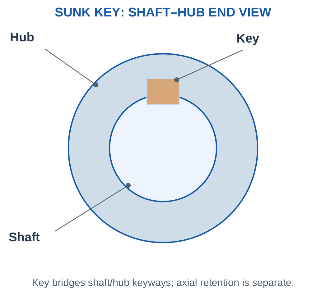
Common Forms
A parallel sunk key has rectangular or square section and engages both members.
A Woodruff key has segmental form seated in a matching shaft recess.
A feather-key arrangement can permit intended axial sliding while transmitting torque when designed for that role.
A spline has multiple longitudinal teeth and is a distinct connection form.
Set screws and interference fits can also provide suitable connections in particular designs, but they are not automatically equivalent to keys.
Axial Retention
A simple parallel key primarily prevents relative rotation.
It does not automatically stop the hub moving axially.
A shoulder, retaining ring, nut or another specified feature can perform that separate function.
An explanation of a keyed gear should therefore identify both its torque path and its axial-retention path.
Worked Problem 3.19: Common Effective Key Length
Problem: Centred usable hub overlap is 30 mm, shaft overlap is 28 mm and straight effective key length is 25 mm.
Step 1: Transmission occurs only over the common usable overlap.
Step 2: For the centred co-located model:
Leffective = min(30, 28, 25) = 25 mm
Step 3: A later uniform-area calculation can use this length only if the model permits it.
Step 4: Axial retention remains a separate requirement.
Worked Problem 3.20: Shaft Overlap Controls
Problem: Centred hub overlap is 40 mm, shaft overlap is 35 mm and key length is 38 mm.
Step 1: Find the region common to all three usable lengths.
Step 2: Leffective = min(40, 35, 38) = 35 mm.
Step 3: The shaft-keyway overlap controls the common length.
Step 4: The result does not establish uniform contact pressure or complete connection capacity.
Worked Problem 3.21: Key Length Controls
Problem: Hub overlap is 24 mm, shaft overlap is 26 mm and effective key length is 22 mm.
Step 1: Use the supplied centred-overlap assumption.
Step 2: Leffective = 22 mm.
Step 3: The straight effective key length is the limiting common length.
Step 4: A separate axial feature is still required if the assembly must prevent axial hub movement.
10. Torque and a Simple Key-Load Model
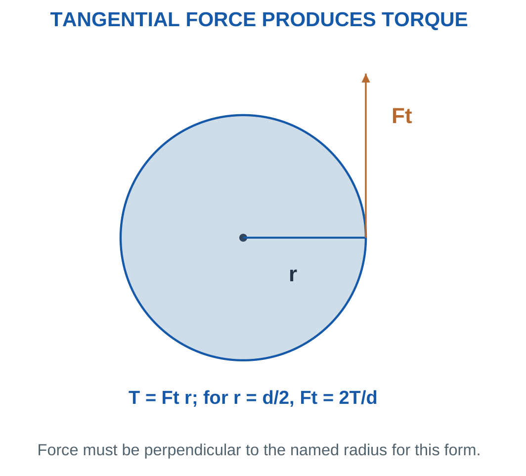
For tangential force Ft at radius r:
T = Ft r
If the effective radius is d/2:
Ft = 2T/d
Use consistent lengths.
A torque in N·mm combines with diameter in mm to give force in N.

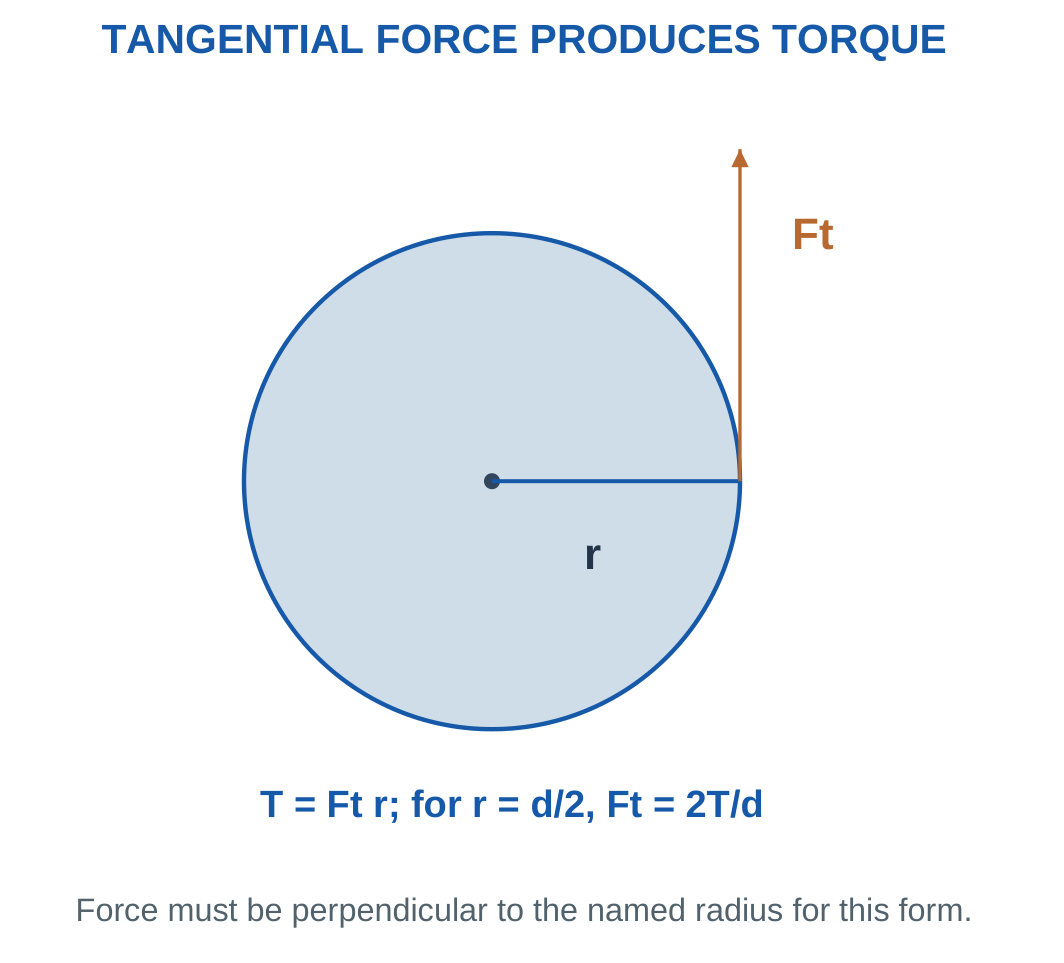
For a rectangular key in the stated uniform model:
Ashear = bL
τavg = Ft/(bL)
If projected contact uses half key thickness:
Acontact = (t/2)L
pavg = Ft/[(t/2)L]
Different Areas
Shear area and projected contact area represent different resisting surfaces.
They should not be interchanged.
Using Ft = T/d instead of 2T/d underestimates force by two in the supplied diameter model.
Real fit, fillets, contact distribution and stress concentrations require additional treatment.
Shaft, Key and Hub

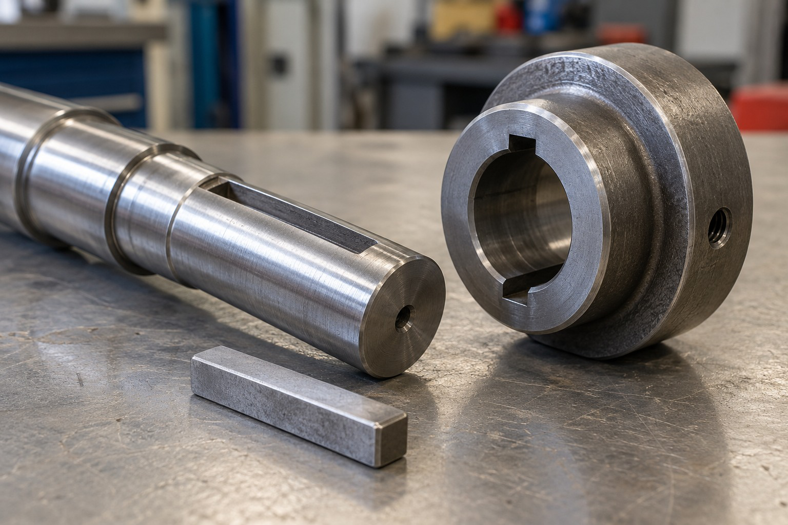
Effective length, nominal shear area and projected contact area are separate geometric quantities.
Worked Problem 3.22: Key at 30 N·m
Problem: Torque is 30 N·m on a 30 mm shaft. Key width is 8 mm, thickness 7 mm and effective length 40 mm.
Step 1: Convert torque:
T = 30000 N·mm
Ft = 2 × 30000/30 = 2000 N
Step 2: Ashear = 8 × 40 = 320 mm².
τavg = 2000/320 = 6.25 MPa
Step 3: Acontact = 3.5 × 40 = 140 mm².
pavg = 2000/140 = 14.2857 MPa
Step 4: 2000 × 15 = 30000 N·mm, recovering torque.
Worked Problem 3.23: Key at 8 N·m
Problem: Torque is 8 N·m, shaft diameter 16 mm, key width and thickness are 5 mm and length is 20 mm.
Step 1: T = 8000 N·mm.
Ft = 2 × 8000/16 = 1000 N
Step 2: Ashear = 100 mm², giving τavg = 10 MPa.
Step 3: Acontact = 50 mm², giving pavg = 20 MPa.
Step 4: The two intensities use different areas. Neither determines keyway concentration or complete shaft-hub capacity.
11. Shafts, Axles and Their Functions
A shaft commonly rotates and transmits torque while supporting gears, pulleys or other mounted parts.
It can carry torsion, transverse loading and axial loading simultaneously.
Steps, shoulders and mounting features locate bearings and hubs.

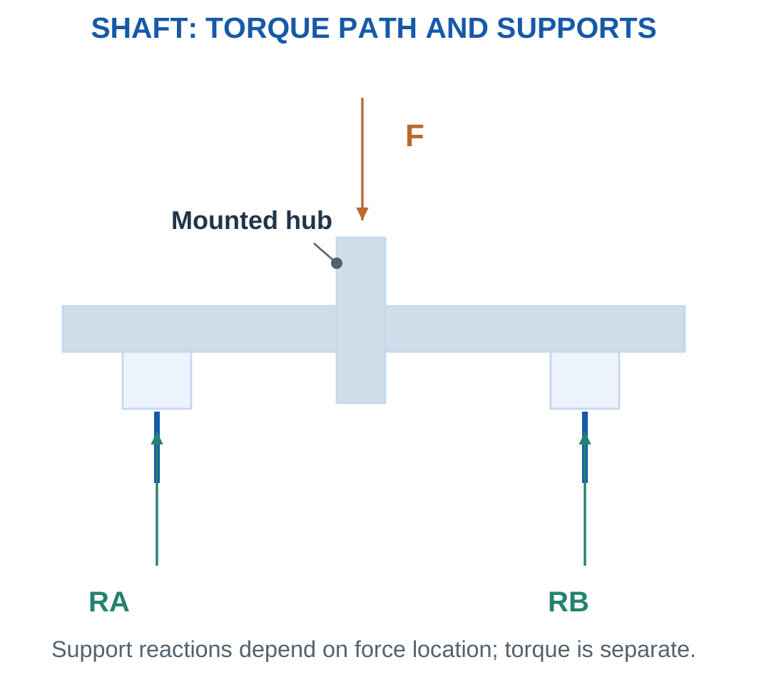
An axle primarily supports rotating members or loads rather than intentionally transmitting useful power between them.
An axle can be stationary or rotating.
The statement that every axle is stationary is therefore too absolute.
A stationary idler support pin is axle-like. A motor output member carrying torque to a pulley is a shaft.
Load Path
Gear tangential force reaches the shaft through its hub connection.
Support forces pass through bearings to the housing.
The bearings do not normally supply the intentional shaft-to-gear torque link.
Shaft stress, deflection, critical speed and fatigue require more detailed models than a layout-length budget.
Worked Problem 3.24: Shaft Layout Length
Problem: Two non-overlapping bearing seats are 10 mm each. Clear spacing totals 60 mm, hub seat is 20 mm and end margins are 8 mm at both ends.
Step 1: Bearing seats total 20 mm.
Step 2: Add spacing and hub seat: 20 + 60 + 20 = 100 mm.
Step 3: End margins add 16 mm.
Total represented length = 116 mm
Step 4: The length budget alone does not determine shaft strength or whether its function is that of a shaft or axle.
Worked Problem 3.25: Another Shaft Layout
Problem: Two bearing seats are 12 mm each, clear spacing is 80 mm, hub seat is 25 mm and end margins are 10 mm each.
Step 1: Bearing-seat total is 24 mm.
Step 2: Add 80 + 25 mm.
Step 3: Add 20 mm margins.
Total = 149 mm
Step 4: This geometric sum assumes the named regions are non-overlapping. A different layout definition could require a different budget.
12. Speed, Torque and Mechanical Power
Convert rotational speed into angular speed:
ω = 2πN/60
Mechanical power is:
P = Tω
Torque is in N·m, angular speed in rad/s and power in W.

At fixed ideal power, lower speed corresponds to greater torque.
For a real transmission:
Pout = ηPin
Therefore:
Tout = ηTin(Nin/Nout)
for the supplied steady boundary and nonzero speeds.
Holding Torque
A static joint can require torque while instantaneous mechanical output power is zero because ω = 0.
The actuator can still consume electrical power or generate heat while holding, depending on its design.
Mechanical output power and electrical input must therefore remain distinct.
Unit Check
Do not substitute rpm directly into P = Tω.
Use:
P = 2πNT/60
when N is in rpm.
Torque multiplication does not create power. It accompanies lower speed and represented losses.
Worked Problem 3.26: Five-to-One Reduction
Problem: Input torque is 2 N·m at 1500 rpm. Reduction is 5 and efficiency is 0.9.
Step 1: ωin = 157.08 rad/s.
Pin = 2 × 157.08 = 314.159 W
Step 2: Nout = 1500/5 = 300 rpm.
Pout = 282.743 W
Step 3: Tout = 0.9 × 2 × 5 = 9 N·m.
Step 4: Output torque times output angular speed gives 282.743 W.
Loss is 31.4159 W.
Worked Problem 3.27: Ten-to-One Reduction
Problem: Tin = 0.5 N·m, Nin = 3000 rpm, reduction = 10 and η = 0.85.
Step 1: ωin = 314.159 rad/s, so Pin = 157.08 W.
Step 2: Nout = 300 rpm and Pout = 133.518 W.
Step 3: Tout = 0.85 × 0.5 × 10 = 4.25 N·m.
Step 4: Loss is 23.5619 W. Output power remains below input despite increased torque.
Worked Problem 3.28: Three-to-One Reduction
Problem: Tin = 8 N·m at 600 rpm, reduction = 3 and η = 0.95.
Step 1: ωin = 62.8319 rad/s.
Pin = 502.655 W
Step 2: Nout = 200 rpm and Pout = 477.522 W.
Step 3: Tout = 0.95 × 8 × 3 = 22.8 N·m.
Step 4: Loss is 25.1327 W.
The power check uses the output speed, not the original input speed.
Worked Problem 3.29: Six-to-One Reduction
Problem: Tin = 1.2 N·m at 1800 rpm, reduction = 6 and η = 0.8.
Step 1: ωin = 188.496 rad/s.
Pin = 226.195 W
Step 2: Nout = 300 rpm and Pout = 180.956 W.
Step 3: Tout = 0.8 × 1.2 × 6 = 5.76 N·m.
Step 4: Loss is 45.2389 W.
Speed, torque and efficiency must belong to the same transmission boundary.
13. Shaft Layout and Bearing Support Forces
A shaft layout positions gears, pulleys, bearings, couplings and locating features.
The arrangement affects support loads and alignment.
For a simple static transverse load between two supports, use the equilibrium relations from engineering mechanics.

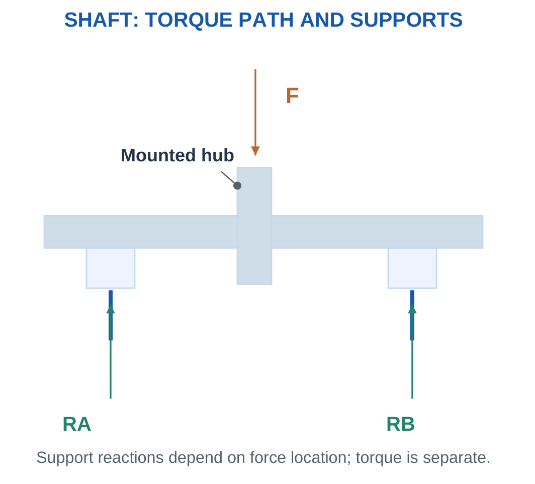
For span L and downward force F at distance a from A:
RB = Fa/L
RA = F − RB
This gives ideal support forces, not bearing life or local shaft stress.
Torque is a separate loading quantity and cannot be added to a reaction force as though both were newtons.
Geometry Matters
An overhung pulley can produce a larger reaction at one support and an opposing signed reaction at another in an appropriate model.
Two bearings do not automatically take half the load.
Real arrangements can include locating and floating functions, preload, axial constraints and housing flexibility.
Worked Problem 3.30: Load Near A
Problem: Bearing centres are 0.3 m apart. A 200 N downward load acts 0.1 m from A.
Step 1: RA + RB = 200 N.
Step 2: RB × 0.3 = 200 × 0.1, so RB = 66.6667 N.
Step 3: RA = 133.333 N.
Step 4: Check about B:
RA × 0.3 = 200 × 0.2 = 40 N·m
The nearer support takes more of the off-centre load.
Worked Problem 3.31: Load Near B
Problem: Span is 0.4 m and 450 N acts 0.25 m from A.
Step 1: RA + RB = 450 N.
Step 2: RB = 450 × 0.25/0.4 = 281.25 N.
Step 3: RA = 168.75 N.
Step 4: 168.75 × 0.4 = 450 × 0.15 = 67.5 N·m.
The reaction distribution follows position, rather than bearing count alone.
Worked Problem 3.32: Central Shaft Load
Problem: Span is 0.5 m and 300 N acts 0.25 m from A.
Step 1: RA + RB = 300 N.
Step 2: RB = 150 N.
Step 3: RA = 150 N.
Step 4: Moment check gives 150 × 0.5 = 300 × 0.25 = 75 N·m.
Equal reactions are justified by the symmetric model.
14. Rigid Couplings: Sleeve and Flange Types
A coupling connects shafts so that torque passes between them.
A rigid coupling has no intentional flexible element for accommodating operating misalignment.
It requires suitable alignment.

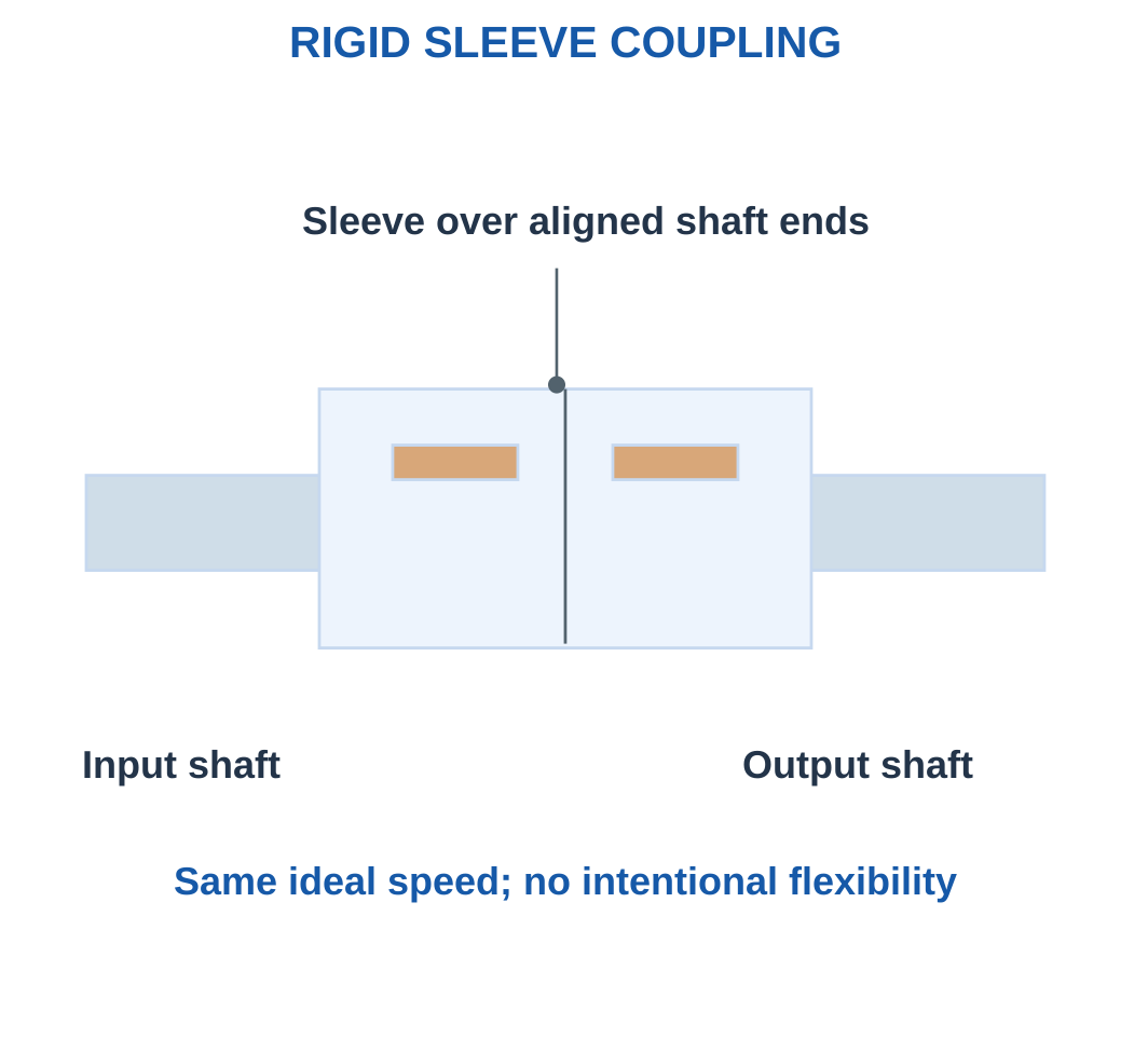
A sleeve or muff coupling surrounds and connects both shaft ends.
A flange coupling uses mating flanges and the specified attachment arrangement.
Some rigid couplings use clamping rather than keys.
The actual torque path must match the design.
Speed and Direction
An ideal rigid connection makes the shafts rotate at the same speed and in the same physical sense along their common axis.
Apparent clockwise direction changes when the observer moves to the opposite end.
Use a common viewing direction.
Flange-Bolt Models
A real flange can transfer torque through clamping friction, bolts in shear or another arrangement.
An exercise explicitly assigning equal tangential shear to bolts uses that model only.
It is not a universal statement about every flange coupling.
Worked Problem 3.33: Four Shear-Loaded Bolts
Problem: Torque is 60 N·m through four equally loaded bolts at radius 40 mm. Smooth bolt diameter is 6 mm with one shear plane.
Step 1: T = 60000 N·mm.
Fbolt = T/(nr) = 60000/(4 × 40) = 375 N
Step 2: A = π × 6²/4 = 28.2743 mm².
Step 3: τavg = 375/28.2743 = 13.2629 MPa.
Step 4: nFr = 60000 N·mm, recovering torque.
A friction-transmitting flange would need a different model.
Worked Problem 3.34: Six Flange Bolts
Problem: T = 120 N·m, n = 6, radius = 50 mm and bolt diameter = 8 mm.
Step 1: Fbolt = 120000/(6 × 50) = 400 N.
Step 2: A = 50.2655 mm².
Step 3: τavg = 400/50.2655 = 7.95775 MPa.
Step 4: 6 × 400 × 50 = 120000 N·mm.
The plane is the supplied smooth single-shear section.
Worked Problem 3.35: Three Flange Bolts
Problem: T = 30 N·m, n = 3, radius = 30 mm and diameter = 5 mm.
Step 1: Fbolt = 30000/(3 × 30) = 333.333 N.
Step 2: A = 19.635 mm².
Step 3: τavg = 16.9765 MPa.
Step 4: The moment sum recovers 30000 N·mm.
The calculation does not establish clamp friction, thread stress or complete coupling capacity.
15. Flexible Couplings and Their Limitations
A flexible coupling connects shafts while accommodating specified limited relative movement through its particular mechanism.
It can reduce forces associated with small alignment errors.
It does not replace appropriate alignment.

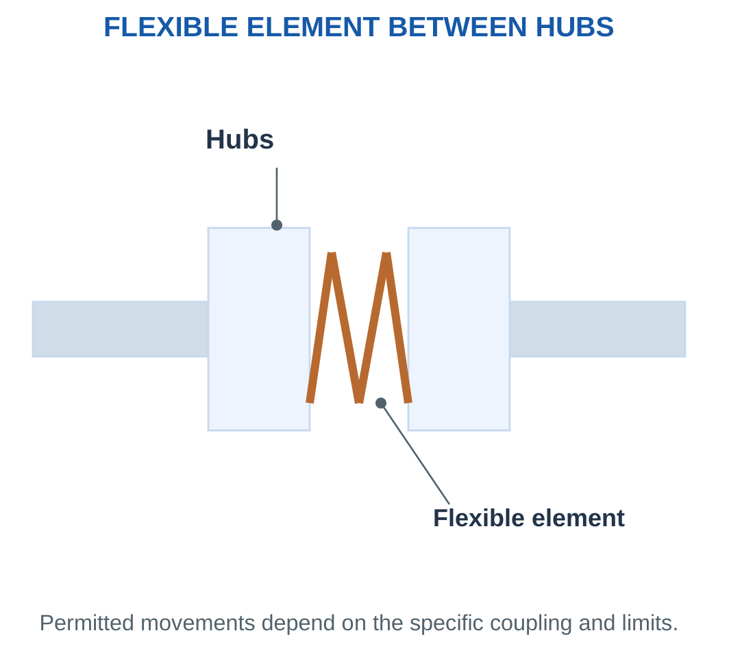
Examples include elastomeric jaw or bush arrangements, bellows, disc couplings and Oldham-type mechanisms.
Their stiffness, backlash, damping and permitted movement differ.
A universal joint can connect intersecting axes in an appropriate arrangement, but instantaneous speed behaviour requires separate consideration.
Precision and Flexibility
A soft-looking element does not automatically provide suitable positioning accuracy.
A robot or printer coupling must combine torque capacity, appropriate accommodation and acceptable lost motion.
Angular, parallel and axial limits should not be assumed equal.
Passing a supplied screen does not establish fatigue life or resonance performance.
Worked Problem 3.36: All Coupling Limits Pass
Problem: Limits are 5 N·m, 2000 rpm, 1° angular error and 0.2 mm offset. Requirements are 3 N·m, 1000 rpm, 0.5° and 0.15 mm.
Step 1: Torque and speed pass.
Step 2: Angular error and parallel offset pass.
Step 3: All four mandatory supplied conditions are satisfied.
Step 4: Axial movement, fatigue, torsional stiffness, resonance and backlash were not assessed.
Worked Problem 3.37: Torque Limit Fails
Problem: Limits are 5 N·m, 1500 rpm, 1° and 0.2 mm. Requirements are 6 N·m, 800 rpm, 0.4° and 0.1 mm.
Step 1: 6 > 5 N·m, so torque fails. Speed passes.
Step 2: Angular and offset checks pass.
Step 3: The complete screen fails because one mandatory condition fails.
Step 4: A favourable speed or alignment value does not compensate for excessive torque under independent limits.
Worked Problem 3.38: Offset Limit Fails
Problem: Limits are 4 N·m, 2000 rpm, 1° and 0.2 mm. Requirements are 2 N·m, 1800 rpm, 0.8° and 0.25 mm.
Step 1: Torque and speed pass.
Step 2: Angle passes, but 0.25 > 0.2 mm offset fails.
Step 3: The candidate fails the supplied screen.
Step 4: Flexible accommodation is limited. It is not permission to ignore alignment.
16. Angular, Parallel and Axial Misalignment
Angular misalignment means the shaft axes have different directions.
Parallel offset means the axes are parallel but laterally displaced.
Axial displacement is relative movement or spacing change along the shaft direction.
A real arrangement can have several simultaneously.

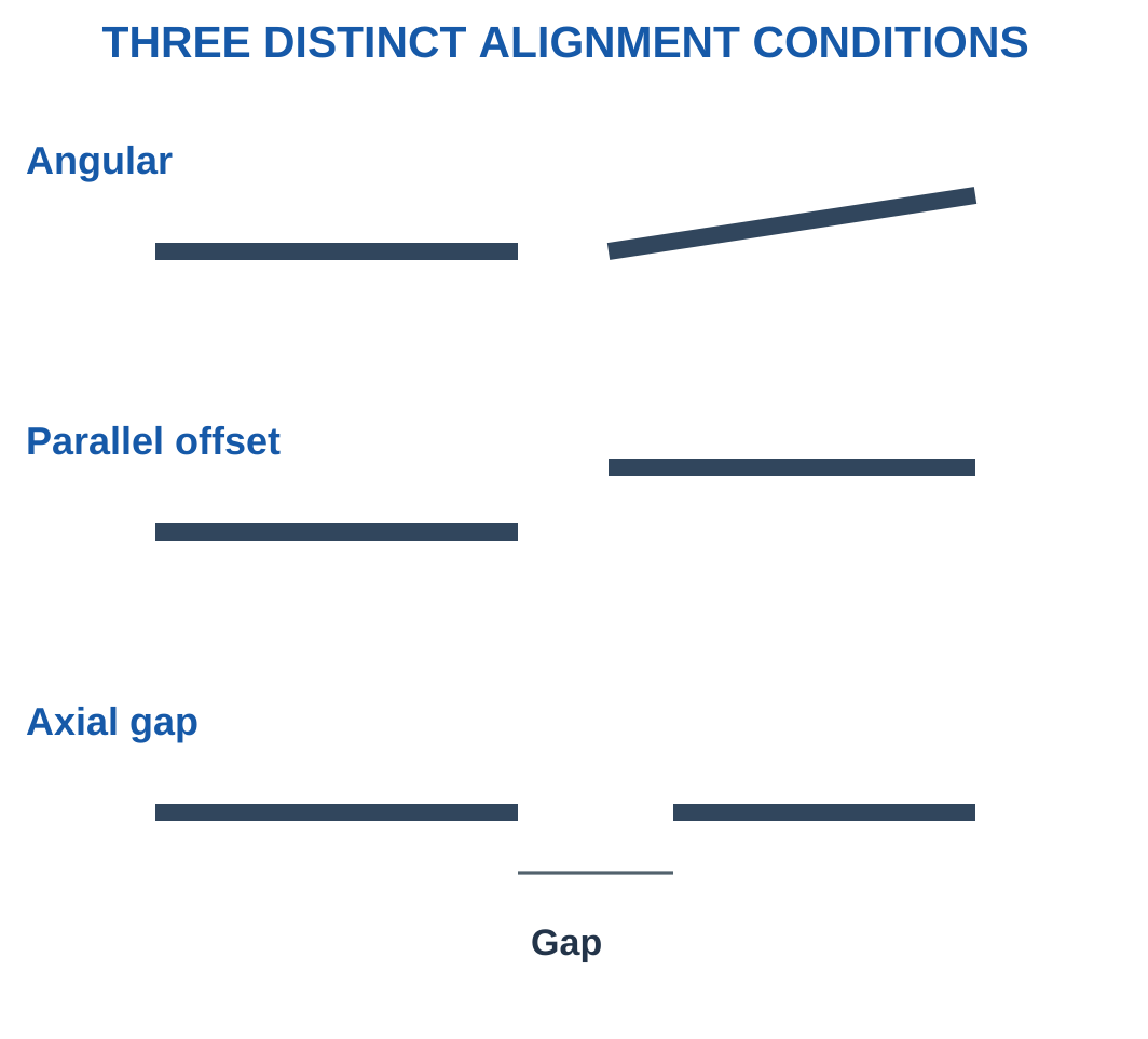
For a stated axis-angle model over reference length L:
e = L tan θ
This gives geometry, not coupling force or permissible error.
A measurement across a diameter is not automatically the same as an axis angle over an axial length.
Operating Alignment
A coupling that turns by hand without load is not proof of acceptable loaded alignment.
Thermal expansion, bearing locations and mounting stiffness affect operation.
Use the specified measurement method.
A favourable angular value cannot offset excessive parallel displacement unless a supplied combined-limit rule explicitly allows it.
Worked Problem 3.39: Offset from 0.2°
Problem: Axis difference is 0.2° over 100 mm. Compare e with a supplied 0.5 mm limit.
Step 1: θ = 0.00349066 rad.
Step 2: e = 100 tan 0.2° = 0.349067 mm.
Step 3: The value is below 0.5 mm.
Step 4: This geometric screen does not predict bearing force or establish the actual coupling’s complete allowable movement.
Worked Problem 3.40: Offset from 0.1°
Problem: θ = 0.1°, L = 150 mm and geometric limit = 0.3 mm.
Step 1: θ = 0.00174533 rad.
Step 2: e = 150 tan 0.1° = 0.2618 mm.
Step 3: The supplied limit passes.
Step 4: The conclusion belongs to this reference-length definition and criterion.
Worked Problem 3.41: Excessive Geometric Offset
Problem: θ = 0.5°, L = 80 mm and limit = 0.4 mm.
Step 1: θ = 0.00872665 rad.
Step 2: e = 80 tan 0.5° = 0.698149 mm.
Step 3: The value exceeds 0.4 mm.
Step 4: Torque capacity and alignment geometry are separate checks. A small transmitted torque does not make this failed criterion pass.
17. Rolling-Bearing Parts and Load Paths
A rolling bearing supports relative motion through rolling elements between raceways.
A common radial bearing contains:
- Inner ring.
- Outer ring.
- Balls or rollers.
- Cage.
- Seals or shields when included.

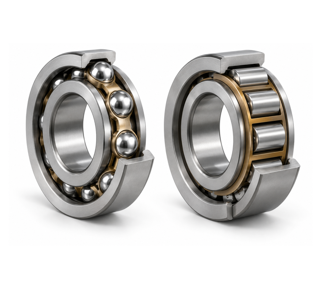

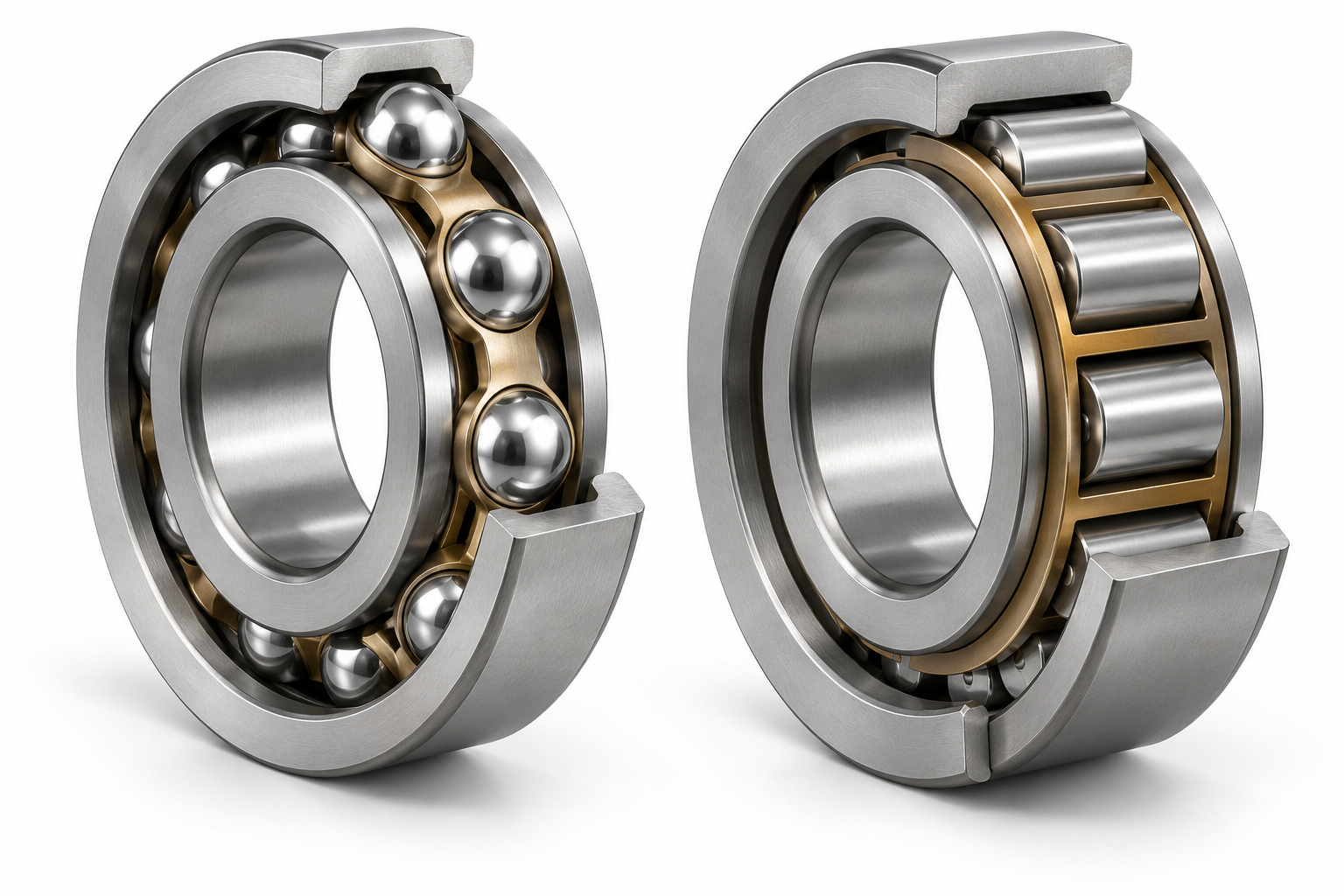

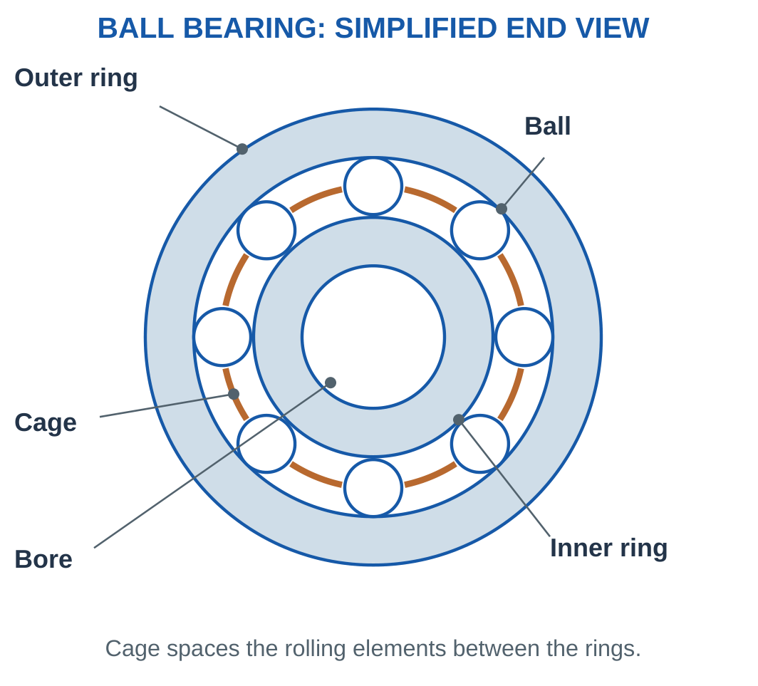
The inner ring often rotates with a shaft while the outer ring remains in a housing, but alternative arrangements exist.
Contacts deform under load.
In a real radial bearing, rolling elements in the loaded region do not necessarily share force equally.
Cage and Structural Load Path
The cage spaces and guides rolling elements.
It is not the intended principal structural path carrying shaft load into the housing.
Rings, raceways and loaded contacts perform that support function.
Rotation and Torque Connection
A bearing supports relative rotation and specified forces.
A key, clamp, fit or other feature connects the shaft to a gear or pulley for useful torque.
The two roles should not be confused.
Worked Problem 3.42: Bearing Envelope
Problem: Bore is 8 mm, outside diameter is 22 mm and width is 7 mm.
Step 1: Outside radius is 11 mm and bore radius is 4 mm.
Step 2: Radial envelope thickness = (22 − 8)/2 = 7 mm.
Step 3: Bore relates to the shaft, outside diameter to the housing and width to axial space.
Step 4: The 7 mm radial envelope includes rings, rolling elements and spaces. It is not automatically ball diameter or one ring’s thickness.
Worked Problem 3.43: Another Envelope
Problem: Bore is 10 mm, outside diameter 30 mm and width 9 mm.
Step 1: Radii are 5 and 15 mm.
Step 2: Radial envelope thickness = 10 mm.
Step 3: Axial occupied width is 9 mm.
Step 4: Envelope dimensions alone do not establish load rating, fit, internal clearance or permitted speed.
18. Ball Bearings: Types and Uses
Ball bearings use spherical rolling elements.
Their nominal raceway contact is often described as point contact.
Under load, elastic deformation creates a finite contact patch.

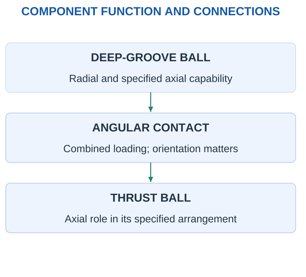
Deep-Groove Ball Bearings
These are common in motors and rotating equipment.
Suitable versions can carry radial and specified axial load under their conditions.
Angular-Contact Ball Bearings
A contact angle and mounting arrangement support combined loading.
A single-row arrangement typically has a preferred axial-load direction.
Thrust Ball Bearings
These serve axial loading in their intended direction and arrangement.
They are not generic radial supports.
Speed and Suitability
Ball bearings are often useful in relatively high-speed, low-friction duties.
Actual limits depend on size, lubrication, sealing, load and temperature.
It is incorrect to claim that every ball bearing is faster or better than every roller bearing.
Drone Application
Drone motors can use ball bearings to support rotating shafts and rotors.
Thrust sharing depends on locating features rather than merely the number of visible bearings.
Worked Problem 3.44: Revolution Count and Speed Screen
Problem: A bearing rotates at 6000 rpm for 20 s. The supplied operating-speed limit is 10000 rpm.
Step 1: Revolutions per second = 6000/60 = 100.
Step 2: Total revolutions = 100 × 20 = 2000.
Step 3: 6000 rpm passes the supplied limit.
Step 4: Rotation count is not a fatigue-life prediction. Load, fit, stiffness and other conditions remain unassessed.
Worked Problem 3.45: Speed Above the Limit
Problem: A bearing rotates at 12000 rpm for 15 s with a supplied limit of 10000 rpm.
Step 1: Rate = 200 revolutions/s.
Step 2: Total = 3000 revolutions.
Step 3: Operating speed exceeds the limit.
Step 4: A short duration does not automatically cancel a mandatory speed criterion in the supplied screen.
19. Roller Bearings: Cylindrical, Needle, Tapered and Spherical
Roller bearings use cylindrical, needle, tapered or barrel-shaped rolling elements.
Nominal line contact becomes a finite loaded region.
Suitable roller arrangements can provide substantial load capability, but actual type and conditions govern selection.

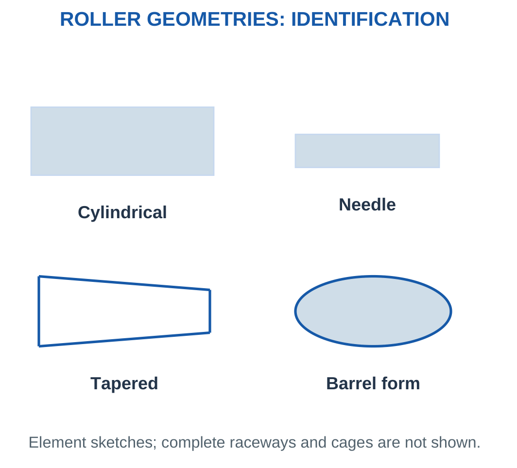
Cylindrical Rollers
These commonly support high radial loading.
Axial capability depends on ring and flange geometry.
Needle Rollers
Slender rollers can fit restricted radial space in suitable arrangements.
The complete raceway and support requirements still matter.
Tapered Rollers
These can support combined radial and axial loads according to orientation and mounting.
Spherical Rollers
These can accommodate specified angular misalignment and substantial loads in their intended arrangement.
Not every roller bearing has the same axial capability or alignment requirement.
Worked Problem 3.46: Radial-Only Supplied Screen
Problem: Limits are Fr ≤ 5000 N, Fa ≤ 0 N and N ≤ 2000 rpm. Requirements are 3000 N radial, zero axial and 1000 rpm.
Step 1: Radial condition passes.
Step 2: Zero axial load satisfies the zero allowance.
Step 3: Speed passes, so the combined independent screen passes.
Step 4: This is not a fatigue-life result or a universal property of every cylindrical roller arrangement.
Worked Problem 3.47: Combined-Load Candidate
Problem: Limits are 4000 N radial, 800 N axial and 2000 rpm. Requirements are 2500 N, 500 N and 1500 rpm.
Step 1: 2500 ≤ 4000 N.
Step 2: 500 ≤ 800 N.
Step 3: 1500 ≤ 2000 rpm. All supplied independent checks pass.
Step 4: Actual combined-load rules can differ from separate inequalities and require type-specific data.
Worked Problem 3.48: Axial Requirement Fails
Problem: Limits are 4000 N radial, 600 N axial and 1800 rpm. Requirements are 2000 N, 900 N and 1200 rpm.
Step 1: Radial load passes.
Step 2: 900 > 600 N, so axial loading fails.
Step 3: Speed passes, but the complete screen fails.
Step 4: A favourable radial value does not compensate for a failed mandatory axial condition.
20. Radial, Axial and Combined Loading
Radial force acts perpendicular to the shaft axis.
Axial or thrust force acts along it.
The axis, rather than page orientation, defines the names.

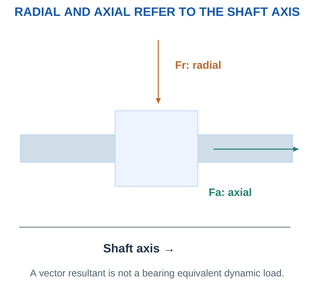
For perpendicular components:
Rgeometric = √(Fr² + Fa²)
This is a vector resultant.
It is not automatically the equivalent dynamic bearing load.
Bearing equivalent-load calculations require type-specific factors and conditions.
Axial Thrust Path
Shoulders, fits and locating features determine which bearing transmits thrust.
A floating function can allow thermal movement.
Two visible bearings do not prove equal axial sharing.
Shaft support reactions and internal rolling-contact distribution are also different levels of analysis.
Worked Problem 3.49: A 300–400 N Resultant
Problem: Fr = 300 N and Fa = 400 N.
Step 1: The components are perpendicular.
Step 2: R = √(300² + 400²) = 500 N.
Step 3: Angle from radial toward axial is atan(400/300) = 53.1301°.
Step 4: Rcos θ and Rsin θ recover the components. Equivalent bearing loading would require another model.
Worked Problem 3.50: A 600–800 N Resultant
Problem: Fr = 600 N and Fa = 800 N.
Step 1: Use the geometric perpendicular-component model.
Step 2: R = 1000 N.
Step 3: θ = 53.1301°.
Step 4: The equal component ratio gives the same angle as the previous problem, while the magnitude doubles.
Worked Problem 3.51: A 1200–500 N Resultant
Problem: Fr = 1200 N and Fa = 500 N.
Step 1: Retain the named radial and axial directions.
Step 2: R = √(1200² + 500²) = 1300 N.
Step 3: θ = atan(500/1200) = 22.6199°.
Step 4: The result is a force vector description rather than a complete selection or rating-life quantity.
21. Lubrication, Seals, Fits and Condition
Lubrication reduces harmful friction and wear through a suitable film.
Lubricant type, amount and replenishment depend on the bearing and service.
More lubricant is not automatically better.
A sealed arrangement can have specific maintenance requirements.

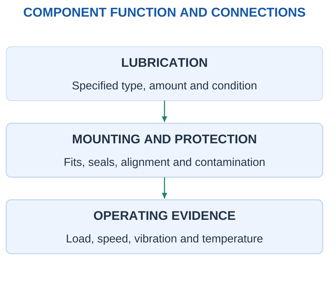
Seals and shields help manage contamination or lubricant retention according to design.
They differ in contact, drag and protection.
Fits and shoulders locate rings and resist unwanted movement under actual loading.
Visible diameter alone is not enough to choose a fit.
Condition Evidence
Noise, vibration, temperature and play can indicate a problem.
One symptom does not uniquely prove bearing failure.
Imbalance, misalignment, poor mounting, lubrication and contact damage can produce related observations.
Interpretation needs operating data and suitable inspection.
Supplied Friction-Torque Model
If resisting torque is supplied:
Ploss = Tfrictionω
This predicts mechanical loss from that torque, not a universal friction coefficient or final bearing temperature.
Temperature also needs a thermal path and surroundings.
Worked Problem 3.52: Friction Loss at 6000 rpm
Problem: Resisting torque is 0.002 N·m at 6000 rpm for 60 s.
Step 1: ω = 628.319 rad/s.
Step 2: Ploss = 0.002 × 628.319 = 1.25664 W.
Step 3: Eloss = 1.25664 × 60 = 75.3982 J.
Step 4: The loss reduces useful mechanical power. It does not by itself determine bearing temperature.
Worked Problem 3.53: Friction Loss at 1500 rpm
Problem: Tfriction = 0.01 N·m and duration is 120 s.
Step 1: ω = 157.08 rad/s.
Step 2: Ploss = 1.5708 W.
Step 3: Eloss = 188.496 J.
Step 4: The energy result is in joules, while the loss rate is in watts.
Worked Problem 3.54: Friction Loss at 12000 rpm
Problem: Tfriction = 0.003 N·m for 30 s at 12000 rpm.
Step 1: ω = 1256.64 rad/s.
Step 2: Ploss = 3.76991 W.
Step 3: Eloss = 113.097 J.
Step 4: A separate thermal model is needed to convert this loss rate into a temperature prediction.
22. Belt Drives and Their Types
A belt drive uses a flexible member around pulleys to transmit motion between separated shafts.
Common types include flat belts, V-belts and synchronous or toothed belts.
A friction belt relies on traction.
A synchronous belt engages compatible teeth.

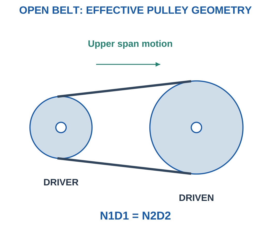
A suitable crossed flat-belt arrangement reverses rotation.
A toothed belt should not be assumed suitable for an arbitrary crossed or twisted arrangement.
Tension and Support Loads
Belt tension supports traction or tooth engagement and also loads the shafts and bearings.
Too little or too much can be harmful.
Increasing tension without a limit is not a universal remedy for lost motion.
Choosing the Model
A no-slip friction-belt relation uses effective or pitch diameters.
A timing belt uses compatible tooth counts and pitch.
Elasticity, tooth compliance, alignment, wear and other connections affect positioning beyond the geometric ratio.
Worked Problem 3.55: Open Belt Speed
Problem: Driver speed is 1200 rpm, driver effective diameter is 50 mm and driven diameter is 100 mm.
Step 1: Equal belt speed gives N1D1 = N2D2.
Step 2: N2 = 1200 × 50/100 = 600 rpm.
Step 3: The normal open arrangement gives the same rotation sense from one side.
Step 4: Slip and creep are neglected. Speed data alone do not establish transmitted torque or bearing load.
Belt and Pulley Drive

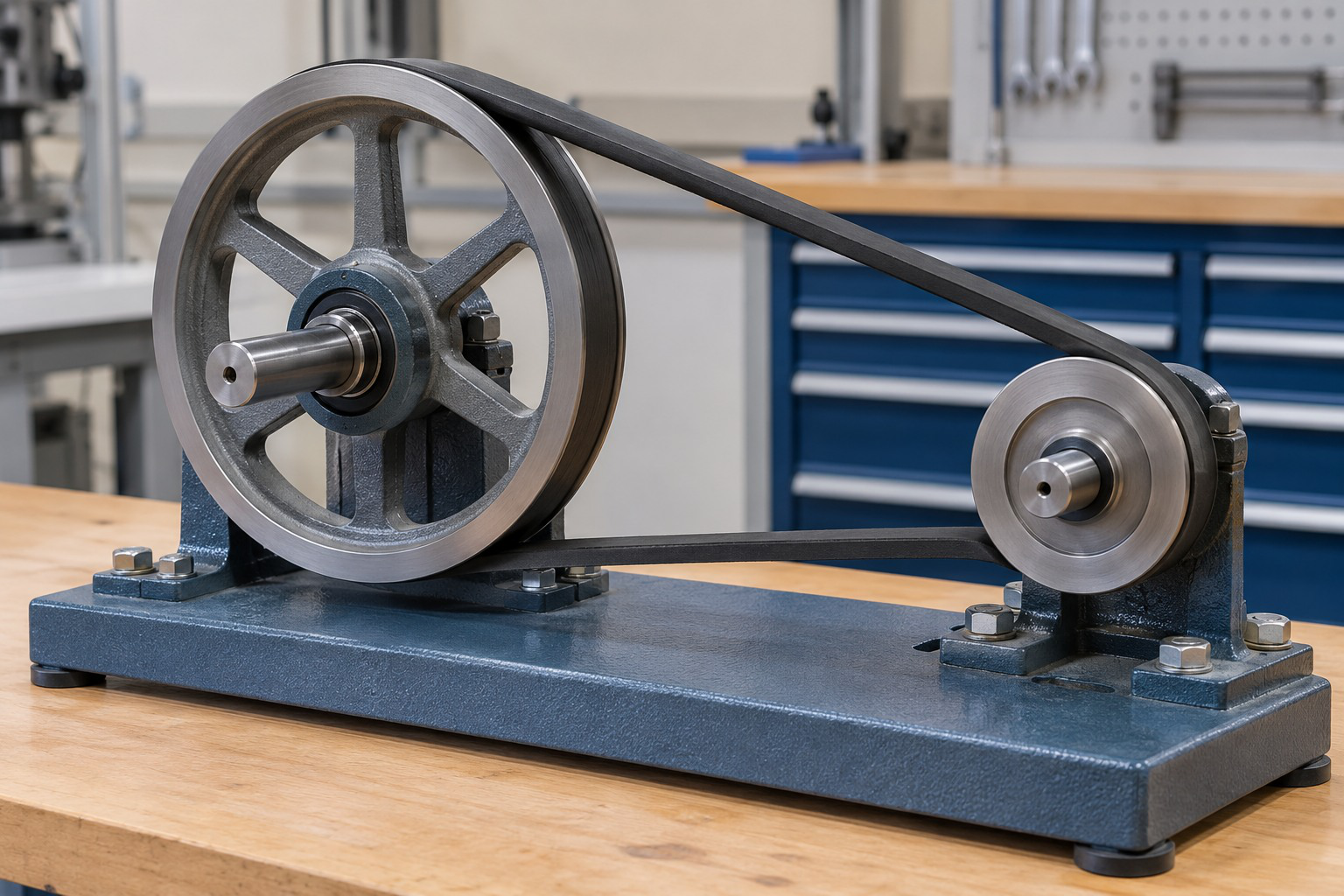
Tension difference transmits power, while span forces also load the shafts.
Direction and ratio depend on the stated layout and geometry.
Worked Problem 3.56: Crossed Flat Belt
Problem: Driver speed is 600 rpm, effective diameters are 60 and 120 mm and the model uses a suitable crossed flat belt.
Step 1: N1D1 = N2D2.
Step 2: N2 = 600 × 60/120 = 300 rpm.
Step 3: The output rotates oppositely from the common viewing side.
Step 4: The crossed-layout conclusion belongs to the stated suitable belt arrangement, rather than every toothed drive.
23. Belt Speed, Speed Ratio and Transmitted Power
For a no-slip model:
v = πDN/60
D is effective diameter in metres, N is rpm and v is m/s.
Equal belt speed gives:
N1D1 = N2D2

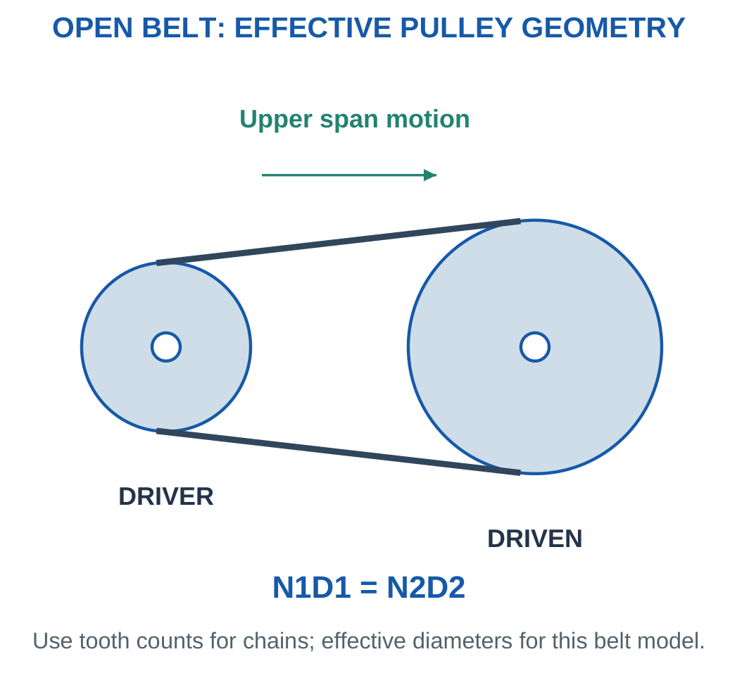
With tight-side tension T1 and slack-side tension T2:
Fdriving = T1 − T2
P = (T1 − T2)v
Tpulley = (T1 − T2)r
The driving force uses the difference, not the sum.
Shaft Loading
For two nearly parallel spans pulling in the same transverse direction, a separate approximation can use their sum.
Exact shaft loading follows the span-force vectors.
Power and support loading therefore use different combinations of the same tensions.
A friction belt can slip or creep. A sound timing drive uses tooth engagement; tooth skipping is a fault outside its ideal no-skip relation.
Worked Problem 3.57: Tension Difference and Shaft Force
Problem: Tight-side tension is 150 N, slack-side tension 50 N, diameter 0.1 m and speed 600 rpm. For the separate support estimate, both spans pull in the same transverse direction.
Step 1: v = π × 0.1 × 600/60 = 3.14159 m/s.
Step 2: Driving force is 100 N and torque is 100 × 0.05 = 5 N·m.
Step 3: P = 100 × 3.14159 = 314.159 W.
Step 4: The parallel-span shaft-force estimate is 150 + 50 = 200 N.
The 200 N support load differs from the 100 N driving force.
Worked Problem 3.58: Higher Tensions
Problem: T1 = 220 N, T2 = 80 N, D = 0.08 m and N = 900 rpm.
Step 1: v = 3.76991 m/s.
Step 2: Fdriving = 140 N and T = 140 × 0.04 = 5.6 N·m.
Step 3: P = 140 × 3.76991 = 527.788 W.
Step 4: Under the stated parallel-span approximation, shaft force is 300 N.
Torque times angular speed gives the same power.
Worked Problem 3.59: Another Belt-Force Model
Problem: T1 = 120 N, T2 = 40 N, D = 0.12 m and N = 500 rpm.
Step 1: v = 3.14159 m/s.
Step 2: Fdriving = 80 N and T = 80 × 0.06 = 4.8 N·m.
Step 3: P = 251.327 W.
Step 4: The parallel-span support estimate is 160 N.
Using tension sum for transmitted power would be incorrect.
24. Timing-Belt Motion in a 3D Printer
A timing belt has teeth at compatible pitch p.
A pulley with z teeth advances the ideal belt by:
Travel per revolution = zp
Its nominal pitch diameter is:
Dpitch = zp/π
The relevant travel comes from pitch circumference, not visible outer diameter.

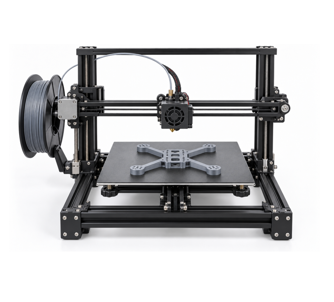

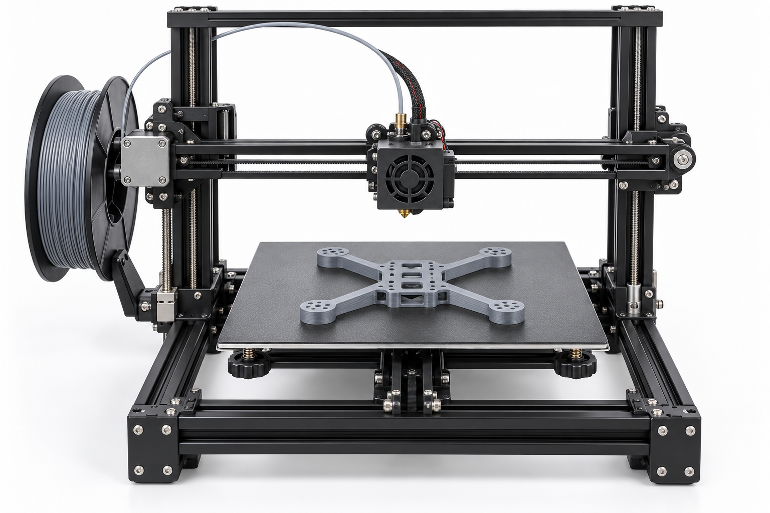

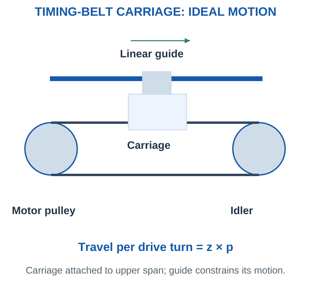
For direct drive:
x = Revolutions × zp
v = Nzp/60
If S commanded increments produce one motor revolution:
Nominal increments/mm = S/(zp)
Command Scale and Accuracy
S may represent full steps or a specified microstep setting.
Smaller command spacing is not proof of equally small physical positioning error.
Elasticity, tooth compliance, guide behaviour, hub slip, missed steps and control affect the actual result.
Idlers redirecting the same ideal belt do not automatically change travel per drive-pulley revolution.
A lead-screw axis instead uses screw lead.
Worked Problem 3.60: Twenty-Tooth Pulley
Problem: z = 20, p = 2 mm, S = 3200 increments/rev, required travel is 120 mm and speed is 120 rpm.
Step 1: Travel/turn = 20 × 2 = 40 mm.
Step 2: Scale = 3200/40 = 80 increments/mm.
Step 3: Commands = 120 × 80 = 9600.
Step 4: v = 120 × 40/60 = 80 mm/s.
Time = 120/80 = 1.5 s
These are ideal kinematic and command values.
Worked Problem 3.61: Sixteen-Tooth Pulley
Problem: z = 16, p = 2 mm, S = 1600, travel = 80 mm and N = 150 rpm.
Step 1: Travel/turn = 32 mm.
Step 2: Scale = 1600/32 = 50 increments/mm.
Step 3: Commands = 4000.
Step 4: v = 150 × 32/60 = 80 mm/s and time = 1 s.
Physical accuracy remains a separate measured property.
Worked Problem 3.62: Twenty-Four-Tooth Pulley
Problem: z = 24, p = 2 mm, S = 3200, travel = 96 mm and N = 90 rpm.
Step 1: Travel/turn = 48 mm.
Step 2: Scale = 3200/48 = 66.6667 increments/mm.
Step 3: Commands = 6400.
Step 4: v = 72 mm/s and time = 1.33333 s.
The exact command count can be obtained using unrounded intermediate values.
25. Chains and Sprockets
A chain drive transmits motion through engagement between links and sprocket teeth.
A common roller chain contains pins, bushes or rollers and plates.
Pitch is the distance between corresponding adjacent pin centres.

A chain uses positive engagement rather than friction-belt traction.
It still requires suitable alignment, sag or tension, lubrication and guarding.
Joint wear can increase effective length.
The phrase chain stretch often describes wear-related length increase rather than uniform permanent extension of every plate.
Direction and Polygonal Action
An ordinary uncrossed two-sprocket drive gives the same rotation sense from a common side.
Tooth counts determine the ideal mean ratio.
Polygonal action can cause cyclic variation about the mean, so positive engagement does not imply perfectly uniform instantaneous speed.
Compatibility
Chain type, pitch, roller dimensions, sprocket form and service must match.
Tooth count alone does not establish fit or load capability.
A chain is not automatically preferable for a quiet, light precision printer axis simply because it has positive engagement.
Worked Problem 3.63: Measured Chain-Length Increase
Problem: One hundred pitch intervals have nominal pitch 12.7 mm. Measured length is 1282.7 mm.
Step 1: Lnominal = 100 × 12.7 = 1270 mm.
Step 2: Increase = 1282.7 − 1270 = 12.7 mm.
Step 3: Percentage increase = 12.7/1270 × 100 = 1%.
Step 4: The value does not prove uniform plastic extension of plates. A service decision needs the specified chain inspection criterion.
Worked Problem 3.64: Eighty Pitch Intervals
Problem: Pitch is 9.525 mm over 80 intervals. Measured length is 769.62 mm.
Step 1: Lnominal = 80 × 9.525 = 762 mm.
Step 2: Increase = 7.62 mm.
Step 3: Percentage increase = 1%.
Step 4: The measurement basis must use the same selected intervals for nominal and measured lengths.
Worked Problem 3.65: No Supplied Length Increase
Problem: There are 120 intervals at 6.35 mm, and measured length is 762 mm.
Step 1: Lnominal = 120 × 6.35 = 762 mm.
Step 2: Increase = 0 mm.
Step 3: Percentage increase = 0%.
Step 4: This measurement does not independently establish every other chain condition, including lubrication, damage or alignment.
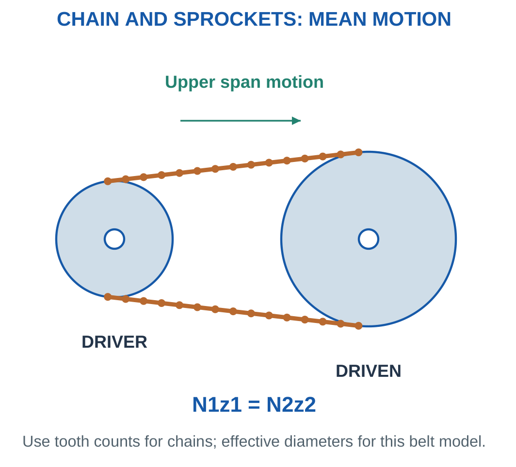
26. Chain-Drive Ratios and Mean Chain Speed
For compatible sprockets:
N1z1 = N2z2
The ideal mean advance per sprocket revolution is:
zp
With pitch in metres:
vmean = zpN/60

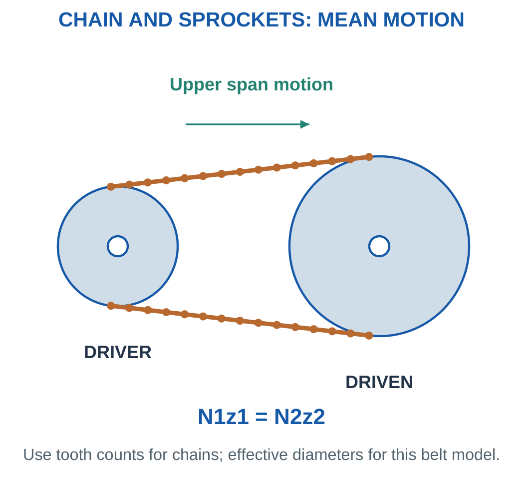
With supplied efficiency:
Pout = ηPin
Tout = Pout/ωout
Ratio alone gives ideal torque multiplication only when losses are neglected.
Pitch Count and Finished Loops
A counted length can be intervals multiplied by pitch when the model defines it that way.
A finished loop also needs the appropriate chain and connector arrangement.
An arbitrary pitch-count result is not automatically a valid physical loop assembly.
Tooth Count and Diameter
Outer sprocket diameter should not be substituted into a friction-pulley equation.
The tooth-count model directly represents the specified mean pitch motion.
Worked Problem 3.66: Fifteen-to-Forty-Five Sprockets
Problem: Driver speed is 900 rpm, tooth counts are 15/45, pitch is 0.0127 m, input power 300 W and efficiency 0.9.
Step 1: Nout = 900 × 15/45 = 300 rpm.
The uncrossed drive gives the same rotation sense.
Step 2: vmean = 15 × 0.0127 × 900/60 = 2.8575 m/s.
Step 3: Pout = 270 W, and ωout = 31.4159 rad/s.
Step 4: Tout = 270/31.4159 = 8.59437 N·m.
Worked Problem 3.67: Twenty-to-Forty Sprockets
Problem: Nin = 600 rpm, teeth are 20/40, pitch is 0.009525 m, Pin = 200 W and η = 0.95.
Step 1: Nout = 300 rpm.
Step 2: vmean = 20 × 0.009525 × 600/60 = 1.905 m/s.
Step 3: Pout = 190 W.
Step 4: Tout = 190/31.4159 = 6.04789 N·m.
The represented losses are applied before calculating output torque.
Chain and Sprockets

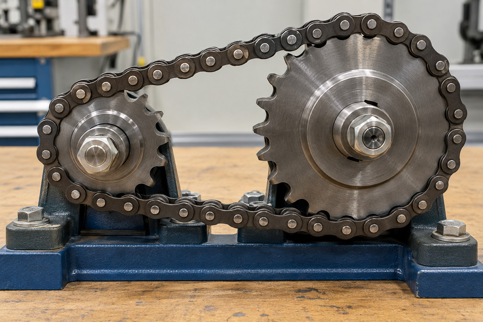
Pitch, measured length increase, mean speed and power describe different checks.
The supplied operating condition determines which relationship applies.
27. Gears and Simple External Meshes
Gears transmit motion through tooth engagement.
A basic external spur pair has parallel shafts and compatible tooth geometry.
The ideal relationship is:
N1z1 = N2z2
One external mesh reverses rotation when viewed from the same side.

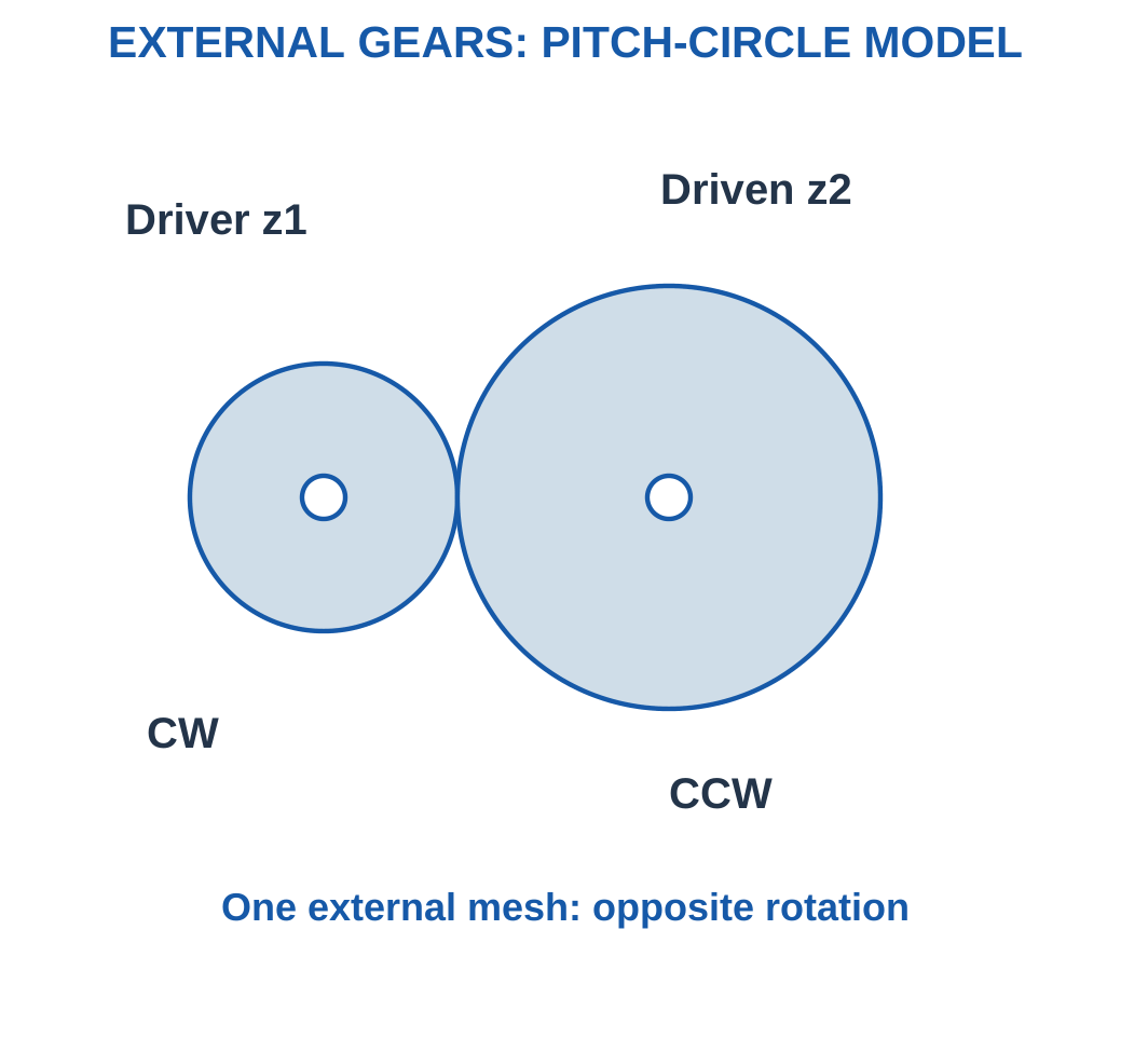
A smaller driver and larger driven gear reduce speed and increase ideal torque.
A larger driver and smaller driven gear increase speed and reduce ideal torque.
With losses, apply efficiency before finding output torque.
Compatible Geometry
Gears need compatible tooth form and pitch and a suitable centre arrangement.
Two touching circles are a kinematic schematic, not a complete manufacturable tooth design.
For this unit:
Reduction = Nin/Nout = zdriven/zdriver
Defining the equation avoids ambiguity in terminology such as velocity ratio.
Worked Problem 3.68: Twenty-to-Sixty Teeth
Problem: Driver/driven counts are 20/60. Input is 1200 rpm at 0.5 N·m and η = 0.95.
Step 1: Reduction = 60/20 = 3.
Step 2: Nout = 400 rpm, opposite input.
Step 3: Tout = 0.95 × 0.5 × 3 = 1.425 N·m.
Step 4: Pin = 62.8319 W and Pout = 59.6903 W.
The power ratio is 0.95.
Worked Problem 3.69: Speed-Increasing Pair
Problem: Counts are 30/15, input is 900 rpm at 1 N·m and η = 0.9.
Step 1: Reduction = 15/30 = 0.5.
Step 2: Nout = 1800 rpm, opposite input.
Step 3: Tout = 0.9 × 1 × 0.5 = 0.45 N·m.
Step 4: Pin = 94.2478 W and Pout = 84.823 W.
A defined reduction below one corresponds here to speed increase.
Worked Problem 3.70: Four-to-One Gear Reduction
Problem: Counts are 18/72, input is 1500 rpm at 0.3 N·m and η = 0.92.
Step 1: Reduction = 4.
Step 2: Nout = 375 rpm, opposite input.
Step 3: Tout = 0.92 × 0.3 × 4 = 1.104 N·m.
Step 4: Pin = 47.1239 W and Pout = 43.354 W.
The reduced speed and losses accompany torque multiplication.
28. Idlers and Compound Gear Trains
A simple train has one relevant gear on each shaft.
An intermediate idler changes layout and the number of external meshes.
Its tooth count cancels from the overall ideal speed ratio between the first and last gears.

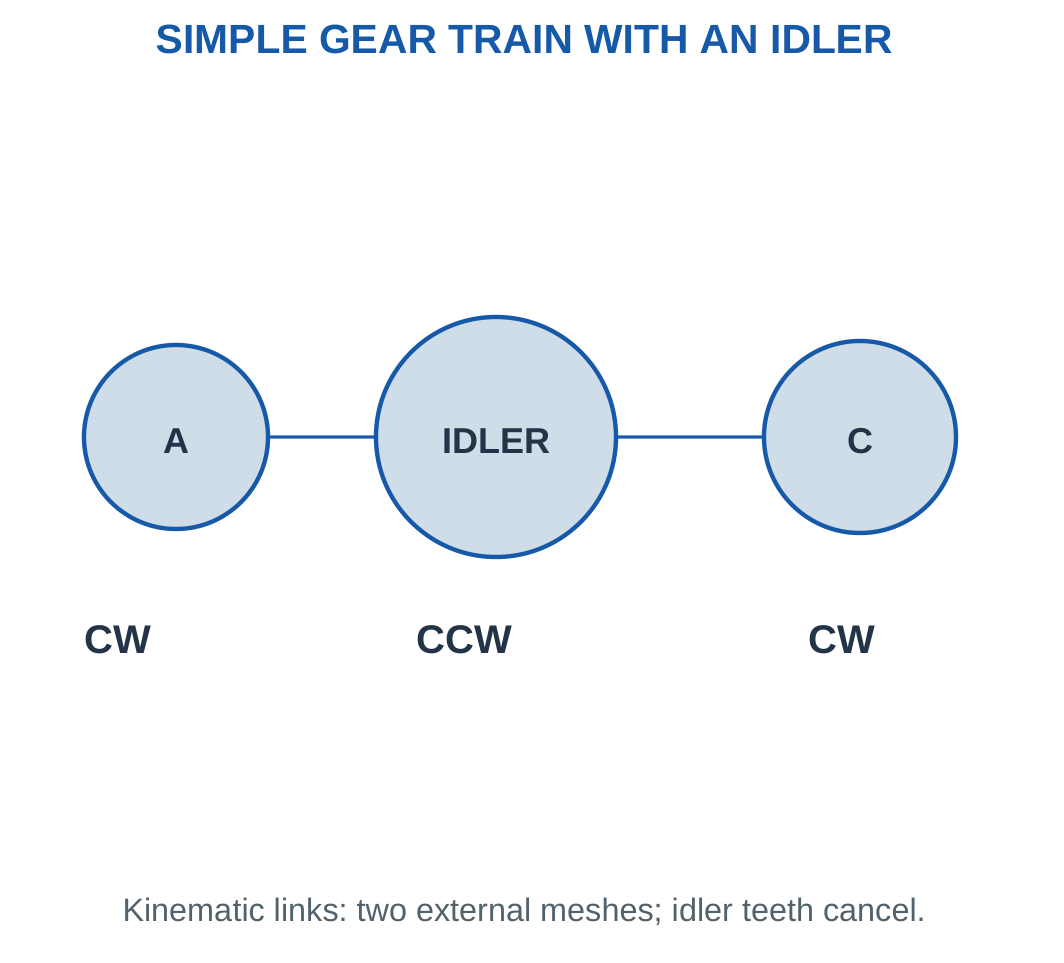
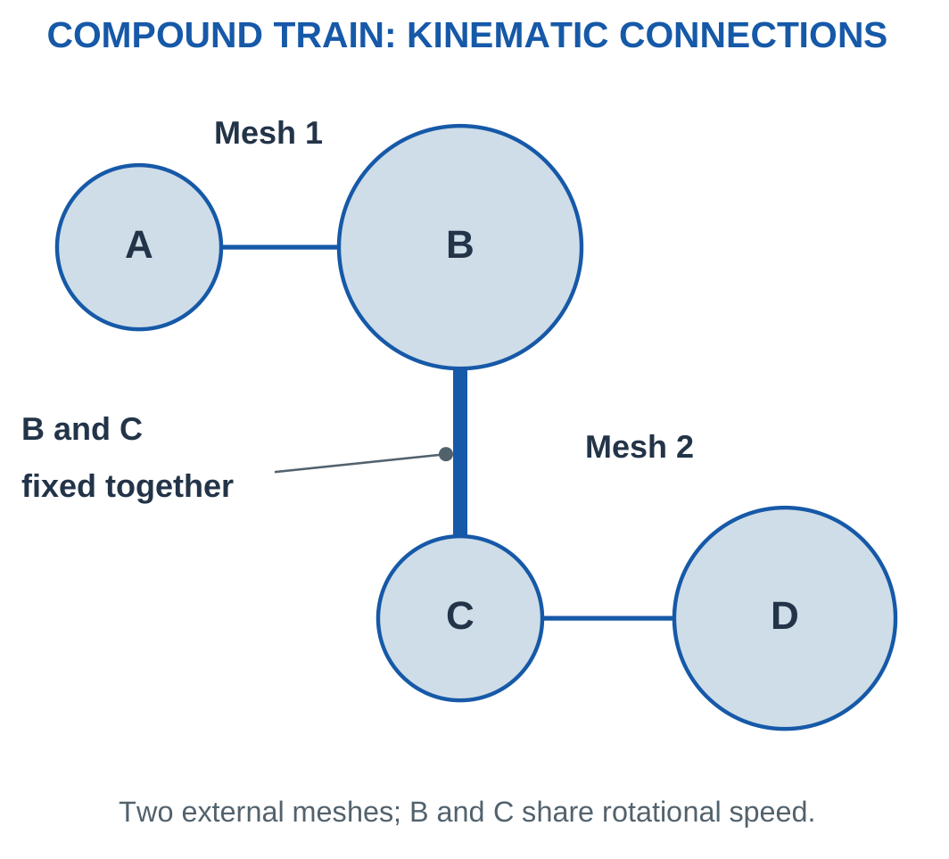
A compound train has two gears fixed to the same intermediate shaft.
For A driving B, C fixed to B and driving D:
NB = NC
Overall reduction = (zB/zA)(zD/zC)
B and C share speed, not necessarily tooth count.

Direction and Efficiency
One external mesh reverses rotation.
Two external meshes restore the input sense along parallel axes viewed from the same side.
A shared shaft does not introduce another reversal.
If separate stage efficiencies are supplied, multiply them.
If complete-train efficiency is supplied, use it once.
Worked Problem 3.71: Compound Reduction of Fifteen
Problem: A/B/C/D have 20/60/15/75 teeth. B and C share a shaft. Input is 1500 rpm at 0.4 N·m and complete-train η = 0.9.
Step 1: Stage reductions are 3 and 5.
Overall reduction = 15
Step 2: NB = NC = 1500/3 = 500 rpm.
Step 3: ND = 500/5 = 100 rpm.
Two external meshes restore input rotation sense.
Step 4: Tout = 0.9 × 0.4 × 15 = 5.4 N·m.
The whole-train efficiency is not applied again at each mesh.
Worked Problem 3.72: Compound Reduction of Twelve
Problem: Counts are 16/48/20/80. Input is 1200 rpm at 0.4 N·m and complete efficiency is 0.85.
Step 1: Stage reductions are 3 and 4.
Overall reduction = 12
Step 2: NB = NC = 400 rpm.
Step 3: ND = 100 rpm, in the input rotation sense under the stated viewing convention.
Step 4: Tout = 0.85 × 0.4 × 12 = 4.08 N·m.
Worked Problem 3.73: Idler Count Cancels
Problem: A 20-tooth input at 600 rpm drives a 35-tooth idler, which drives an 80-tooth output. Both meshes are external.
Step 1: Nidler = 600 × 20/35 = 342.857 rpm, opposite input.
Step 2: Nout = 342.857 × 35/80 = 150 rpm.
Step 3: Algebra gives:
Nout = Nin × zinput/zoutput
Step 4: Two external reversals restore input sense.
The idler still determines its own speed and affects layout even though its count cancels from the end-to-end magnitude ratio.
29. A Robotic Joint: Reduction, Torque and Precision
A robot joint can contain a motor, reducer, support bearings, shaft-hub connections and a housing.
The motor supplies input torque and speed.
Reduction gives lower output speed and greater torque, with output power reduced by losses.

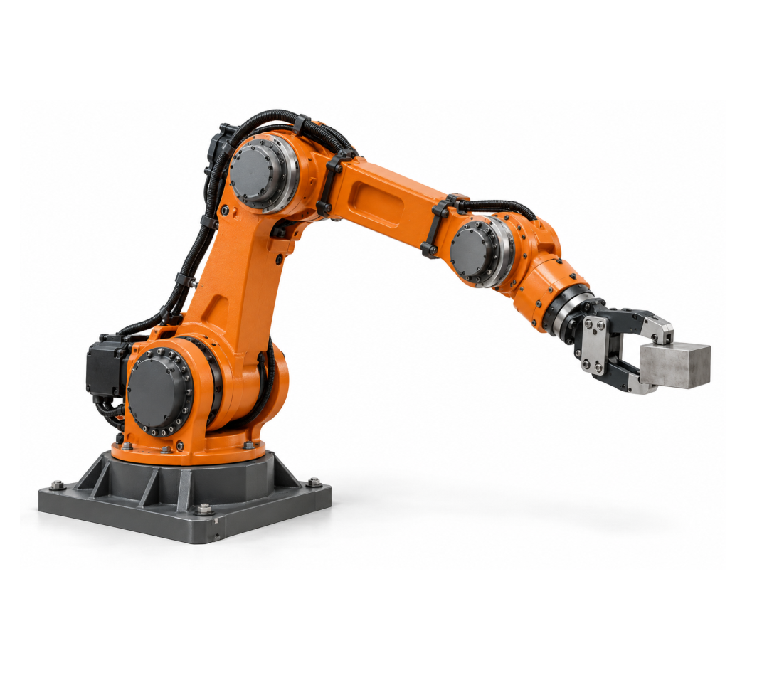

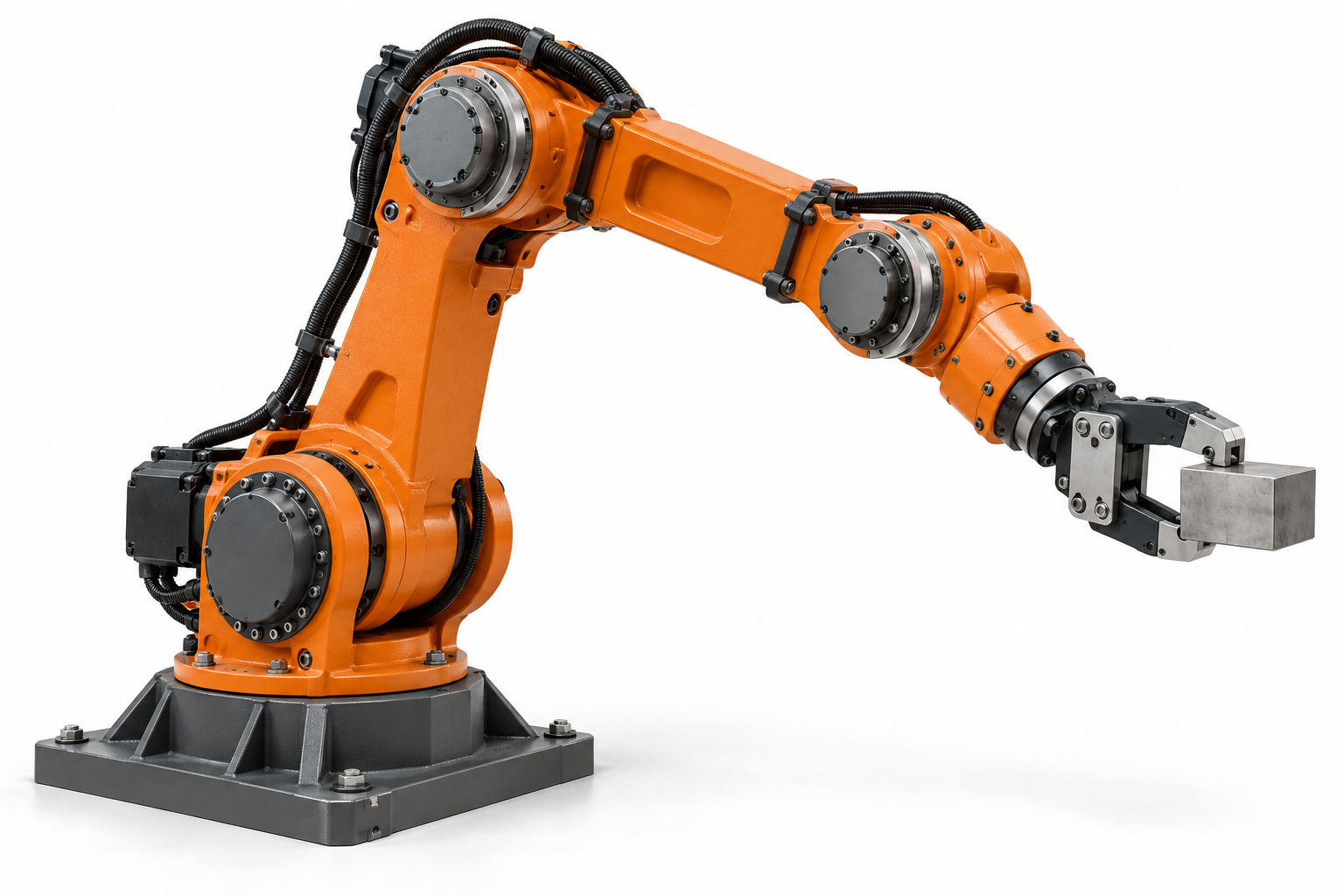

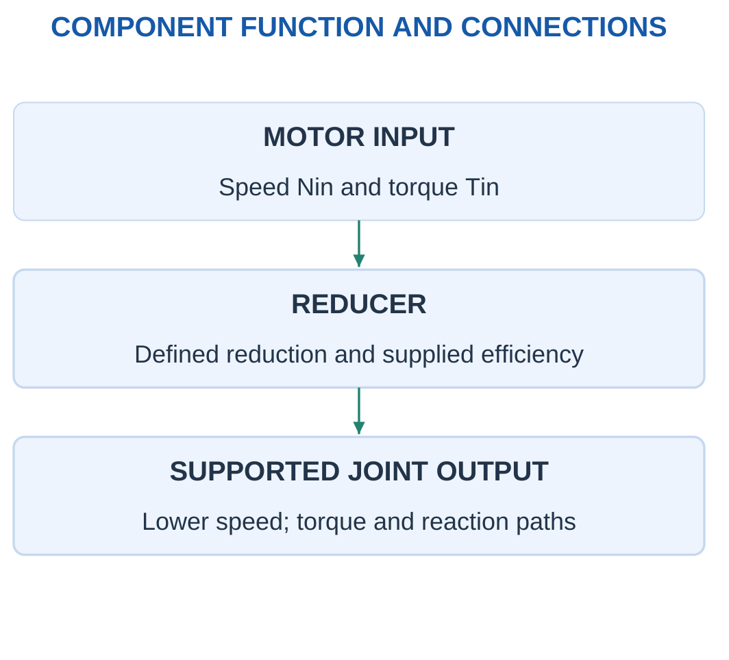
For the stated steady boundary:
Tout = ηTin × Reduction
A simple load requirement can use force times perpendicular arm.
Link weight, acceleration and changing configuration need additional terms when relevant.
Precision
Backlash is lost motion associated with clearance during reversal in the stated mechanism.
Elastic deflection is load-dependent deformation.
They are not identical.
A nominal ratio does not guarantee exact endpoint position.
Keys, clamps, bearings, housing stiffness and control all influence the complete result.
Worked Problem 3.74: Joint Torque from a 20 N Force
Problem: Force is 20 N at perpendicular arm 0.3 m. Output speed is 30 rpm, reduction 20 and efficiency 0.8.
Step 1: Tout = 20 × 0.3 = 6 N·m.
Step 2: Tin = 6/(0.8 × 20) = 0.375 N·m.
Step 3: Nin = 30 × 20 = 600 rpm.
Pout = 18.8496 W
Pin = 23.5619 W
Step 4: Pout/Pin equals 0.8.
These are steady requirements rather than peak, stall or complete duty-cycle ratings.
Worked Problem 3.75: Joint Torque from a 35 N Force
Problem: Force is 35 N at 0.2 m, output speed 40 rpm, reduction 15 and efficiency 0.85.
Step 1: Tout = 7 N·m.
Step 2: Tin = 7/(0.85 × 15) = 0.54902 N·m.
Step 3: Nin = 600 rpm.
Pout = 29.3215 W
Pin = 34.4959 W
Step 4: The ratio agrees with the supplied efficiency.
Additional dynamic and joint requirements remain outside this simple calculation.
Worked Problem 3.76: Joint Torque from a 15 N Force
Problem: Force is 15 N at 0.4 m, output speed 20 rpm, reduction 25 and efficiency 0.9.
Step 1: Tout = 6 N·m.
Step 2: Tin = 6/(0.9 × 25) = 0.266667 N·m.
Step 3: Nin = 500 rpm.
Pout = 12.5664 W
Pin = 13.9626 W
Step 4: Increased reduction lowers the required steady input torque for the specified output, but raises input speed accordingly.
30. Drone-Motor Ball Bearings and Rotating Assemblies
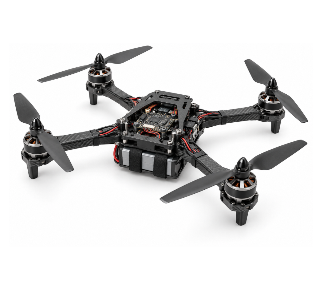
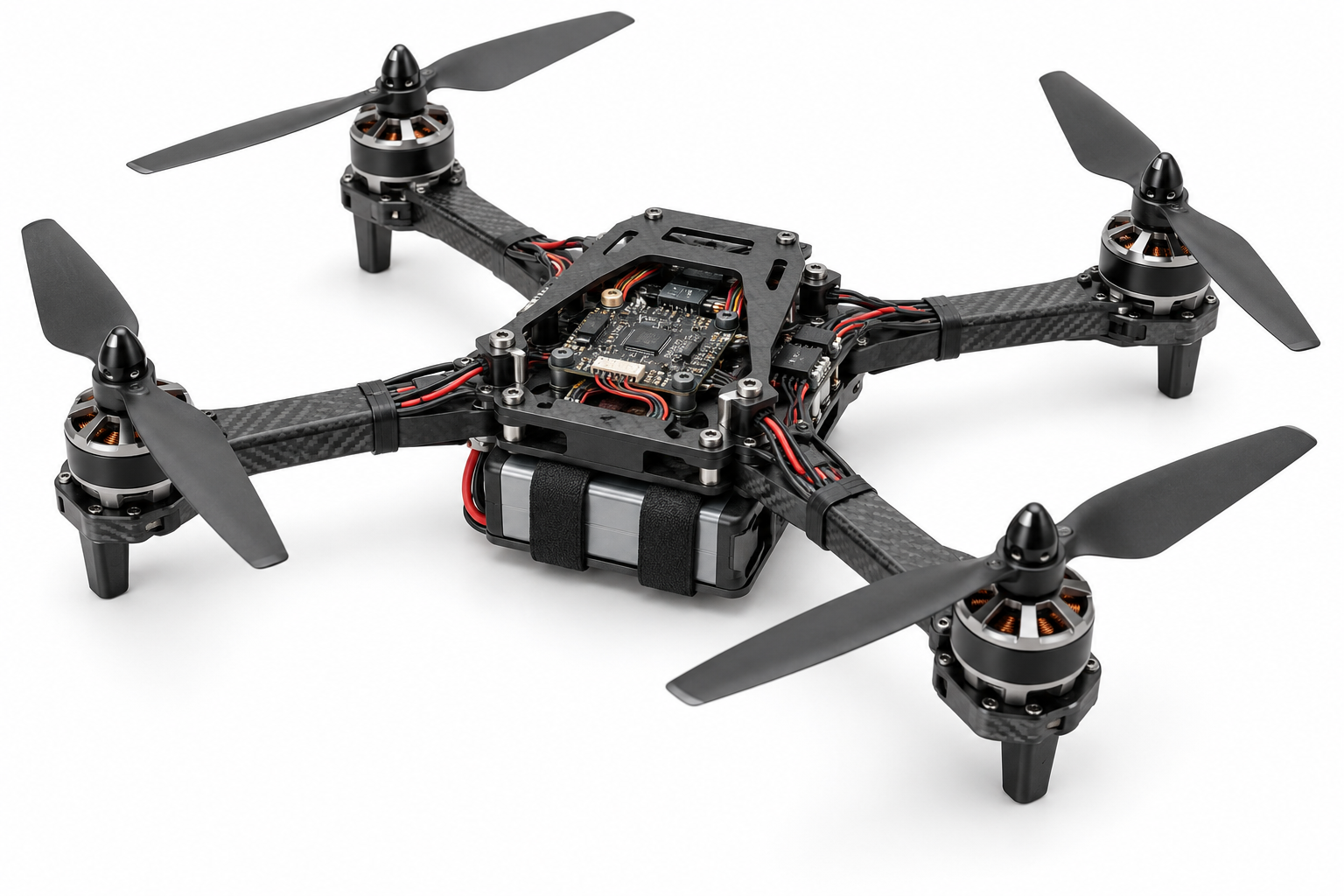
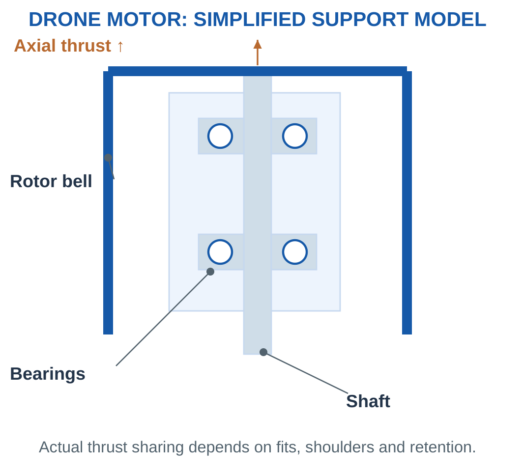
A drone motor needs stable support with suitable friction, speed capability, stiffness and mass.
Ball bearings are common, but actual load paths, preload and locating features depend on the product.



Imbalance
For a supplied eccentric point-mass model:
Fimbalance = meω²
where m is represented eccentric mass and e is eccentricity.
Doubling speed multiplies force by four.
The direction of this transverse force rotates with the eccentricity.
It is not automatically the static force on each bearing.
Thrust and Support
Propeller thrust acts along the motor axis.
Shoulders, fits and retention determine which bearing carries it.
Two bearings do not automatically share thrust equally.
Lubrication, contamination, mounting, thermal conditions and balance affect service.
Worked Problem 3.77: Imbalance at 10000 rpm
Problem: m = 0.002 kg, e = 0.2 mm and N = 10000 rpm. Find force and its value at twice speed.
Step 1: e = 0.0002 m and ω = 1047.2 rad/s.
Step 2: F = 0.002 × 0.0002 × 1047.2² = 0.438649 N.
Step 3: At twice speed:
Fnew = 4F = 1.7546 N
Step 4: Support geometry and dynamics are needed to determine individual bearing forces.
Worked Problem 3.78: Imbalance at 12000 rpm
Problem: m = 0.001 kg, e = 0.15 mm and N = 12000 rpm.
Step 1: e = 0.00015 m, ω = 1256.64 rad/s.
Step 2: F = 0.236871 N.
Step 3: At double speed, Fnew = 0.947482 N.
Step 4: The speed-squared trend belongs to the supplied mass-eccentricity model, not a complete rotor-dynamic assessment.
Worked Problem 3.79: Imbalance at 8000 rpm
Problem: m = 0.003 kg, e = 0.1 mm and N = 8000 rpm.
Step 1: e = 0.0001 m, ω = 837.758 rad/s.
Step 2: F = 0.210552 N.
Step 3: At double speed, Fnew = 0.842206 N.
Step 4: The result is a rotating excitation. It does not by itself establish bearing life or permitted motor speed.
31. Comparison Tables and Formula Sheet
Component Functions
| Component | Main Role | Important Distinction |
|---|---|---|
| Bolt or screw | Detachable joining or retention | Identify the actual mating thread |
| Washer | Specified contact or spacing function | Plain washer is not universal positive locking |
| Key | Shaft-hub torque connection | Axial retention can require another feature |
| Shaft | Torque transmission and support of mounted parts | Can carry bending and axial loads |
| Axle | Primarily support | Can be stationary or rotating |
| Rigid coupling | Connection of aligned shafts | No intended flexible accommodation element |
| Flexible coupling | Connection with limited accommodation | Torque, speed and movement limits still apply |
| Ball bearing | Rolling support using balls | Type determines load capability |
| Roller bearing | Rolling support using rollers | Different forms have different functions |
| Friction belt | Traction-based pulley transmission | Effective diameters and slip assumptions matter |
| Timing belt | Toothed transmission | Compatible pitch and tooth count matter |
| Chain | Link-to-sprocket engagement | Mean motion differs from perfectly uniform instantaneous motion |
| Gear train | Meshed-tooth transformation | External meshes reverse direction |
Introductory Formulae
| Relation | Conditions |
|---|---|
| Lead = Starts × Pitch | Compatible thread geometry |
| Screw travel = Turns × Lead | Stated motion constraints |
| Screw speed = N × Lead / 60 | Lead in mm/rev gives mm/s |
| σavg = F/A | Supplied central direct-load model |
| T = Ft r | Tangential force at named radius |
| Ft = 2T/d | Effective radius d/2 |
| Key shear = Ft/(bL) | Explicit uniform effective area |
| Projected contact pressure = Ft/[(t/2)L] | Supplied half-thickness model |
| ω = 2πN/60 | N in rpm |
| P = Tω | Same-axis mechanical power |
| Pout = ηPin | Defined transmission boundary |
| Tout = ηTin Nin/Nout | Steady nonzero-speed model |
| N1D1 = N2D2 | No-slip effective-diameter belt model |
| v = πDN/60 | D in metres |
| Pbelt = (T1 − T2)v | Supplied tight/slack tension model |
| Timing travel per turn = zp | Compatible pitch and teeth |
| Increments/mm = S/(zp) | Direct timing axis |
| N1z1 = N2z2 | Ideal gear or mean chain relation |
| Mean chain speed = zpN/60 | Pitch in metres gives m/s |
| Compound reduction = Product of stage reductions | Shared gears fixed on each shaft |
| Ploss = Tfrictionω | Supplied resisting torque |
| Fimbalance = meω² | Supplied eccentric point-mass model |
Numerical Method
Identify input and output.
Define the reduction.
Use a common viewing direction.
Convert units.
Apply the actual mechanical connection.
Include supplied efficiency at the correct boundary.
Check power and physical trends.
A kinematic result should not be expanded into an unsupported full strength, life or accuracy claim.
32. Short Questions with Clear Answers
1. What Is the Difference Between a Bolt and a Screw?
A common teaching distinction is a through-bolt with a separate nut versus a screw engaging a tapped or formed receiving thread.
Naming can depend on the standard.
Identify the actual mating arrangement rather than relying on appearance alone.
2. What Does a Washer Do?
It provides its specified bearing, spacing or retention-related function.
A plain washer can spread contact and protect a surface.
It is not automatically a positive anti-loosening device.
3. How Do Pitch and Lead Differ?
Pitch is adjacent-thread axial spacing.
Lead is advance per relative revolution.
For a single-start thread, they are equal. For multiple starts:
Lead = Starts × Pitch
4. Why Is Tightening Torque Different from Clamp Force?
Torque is a turning effect, while clamp force is an axial force.
They have different units.
Their relationship depends strongly on thread and bearing friction and the joint model.
5. What Does a Key Connect?
It connects a shaft and hub to prevent relative rotation and transmit torque.
A separate feature can be needed for axial retention.
The keyway arrangement defines how the contact occurs.
6. Is Every Axle Stationary?
No.
An axle’s main function is support rather than intended useful power transmission.
It can be stationary or rotating depending on the assembly.
7. How Do Rigid and Flexible Couplings Differ?
A rigid coupling requires suitable alignment without an intentional flexible accommodation element.
A flexible type allows specified limited motion through its mechanism.
It still has speed, torque and alignment limits.
8. Do Bearings Normally Provide the Shaft-to-Pulley Torque Connection?
Normally the intentional torque link is a key, clamp, fit or other specified hub feature.
Bearings support relative rotation and loads between their mounted members.
These are different functions.
9. Are Loaded Ball Contacts Literally Points?
No.
Point contact is a nominal geometric description.
Elastic deformation creates a finite loaded patch.
Roller line contacts likewise become finite contact regions.
10. Can Every Roller Bearing Carry Axial Thrust?
No.
Axial capability depends on roller type, ring geometry, orientation and mounting.
A cylindrical radial arrangement and a tapered roller arrangement cannot be assigned identical functions without checking the design.
11. Why Is the Geometric Resultant Not Automatically Equivalent Bearing Load?
√(Fr² + Fa²) is a vector magnitude.
Equivalent bearing-load calculations use type-specific factors and operating conditions.
The geometric result alone is not a complete rating-life input.
12. Does an Open Belt Reverse Rotation?
For the normal parallel-shaft open arrangement viewed from the same side, rotation sense is the same.
A suitable crossed flat-belt arrangement reverses it.
The viewing convention must remain consistent.
13. What Travel Does a Timing Pulley Give per Turn?
In the ideal no-skip model:
Travel = zp
Use compatible belt pitch and pulley teeth.
Visible outer diameter is not the required pitch-circumference basis.
14. Does an Idler Count Change a Simple Train’s Overall Ratio?
The count cancels from the ideal end-to-end ratio.
The idler still affects its own speed, layout and number of external meshes.
It can therefore affect the direction relationship.
15. Why Does a Drone Rotor Need Good Balance?
The supplied model gives:
F = meω²
Force rises strongly with speed.
Balance supports smoother loading, while actual bearing and motor limits still require complete operating information.
33. Complete Examination Answers
1. Explain Threaded Fasteners and a Correctly Interpreted Joint
A common bolted joint uses a headed externally threaded member passing through clearance holes and engaging a separate nut.
A screw commonly engages a tapped or formed receiving thread.
Actual naming depends partly on standards, so the mating arrangement should be identified.
Washers provide specified contact or spacing functions. A plain washer alone does not establish positive resistance to loosening.
Tightening develops preload: fastener tension is balanced by compression in the joined stack.
Grip and usable thread engagement are separate dimensions.
A screw can bottom in a blind hole without producing the intended clamp.
Pitch is adjacent-thread spacing. Lead is advance per relative revolution and equals starts multiplied by pitch.
Installation torque is not axial force. Friction and joint conditions affect their relationship.
Average stress uses the supplied area and sharing model.
Real behaviour also depends on engagement, receiving material, joint stiffness, eccentricity, service and retention.
An introductory force-area check therefore explains one model rather than certifying the complete assembly.
2. Explain Keys and Compare Them with Other Retention Features
A key prevents relative rotation between shaft and hub through matching keyways.
A parallel sunk key occupies portions of both members.
A Woodruff key has segmental form.
A suitable feather-key arrangement can allow intended axial sliding while transmitting torque.
A spline is a distinct multiple-tooth connection.
For the supplied diameter model:
Ft = 2T/d
Uniform rectangular-key shear uses:
τavg = Ft/(bL)
A separately specified contact model can use:
pavg = Ft/[(t/2)L]
The areas describe different surfaces.
Real contact, fit and keyway stress concentrations require more analysis.
A basic key does not automatically retain a hub axially. A shoulder, nut or retaining ring can provide that role.
Set screws and interference fits can connect hubs in appropriate designs, but they are not universally interchangeable with keys.
A complete explanation separates torque transmission from axial retention.
3. Explain Shafts, Axles and Couplings as One Assembly
A shaft commonly rotates and carries useful torque while supporting gears and pulleys.
It can experience torsion, transverse force and axial force simultaneously.
An axle mainly provides support and may be stationary or rotating.
A coupling connects shafts.
Rigid sleeve and flange types need suitable alignment.
Flexible types use specific mechanisms to accommodate limited angular, parallel or axial movement.
Their stiffness, damping and backlash differ.
Bearings support the shafts and transfer reactions to housings.
Keys, clamps or other attachments connect hubs for torque transmission.
A supplied two-support model gives reactions through equilibrium.
Mechanical power follows:
P = Tω
Neither a reaction calculation nor speed ratio establishes shaft fatigue, critical speed, deflection or bearing life.
A labelled assembly should show which component carries torque and which component transfers support force to the frame.
4. Compare Ball and Roller Bearings without Absolute Claims
A rolling bearing commonly contains rings, raceways, rolling elements and a cage.
Seals or shields are present where required.
Balls have nominal point contact that becomes a finite patch under load.
Rollers have nominal line contact that becomes a finite region.
The cage spaces and guides the elements rather than carrying the principal shaft-to-housing load.
Deep-groove ball bearings are common radial supports with specified axial capability.
Angular-contact types suit combined loading in an appropriate orientation.
Thrust ball bearings serve axial roles.
Cylindrical rollers commonly provide radial capacity. Needle rollers suit restricted radial space. Tapered rollers can carry combined loads. Spherical rollers permit specified angular accommodation.
Selection considers direction, magnitude, speed, space, stiffness, fit, lubrication, contamination and temperature.
Not every ball bearing is faster than every roller bearing.
Not every roller bearing carries axial thrust.
The mounting arrangement also determines the actual thrust path.
5. Explain Belt and Chain Transmission and Their Equations
A friction belt transmits through traction at pulleys.
A synchronous belt engages teeth.
For the supplied no-slip friction model:
N1D1 = N2D2
Use effective or pitch diameters.
Belt power is:
P = (T1 − T2)v
The driving force uses tension difference.
The support load depends on the vector combination of span forces and can involve their sum in a stated approximation.
An open belt gives the same rotation sense from a common side. A suitable crossed flat belt reverses it.
A chain engages matching sprocket teeth.
The ideal mean relation is:
N1z1 = N2z2
and mean advance per revolution is zp.
Wear, lubrication, alignment and polygonal action affect service.
Positive engagement does not eliminate every cyclic speed variation.
For either drive, apply supplied efficiency to output power and calculate torque from the associated output speed.
6. Explain a Timing-Belt Axis in a 3D Printer
A motor drives a compatible toothed pulley and belt.
A carriage attached to one span is constrained by a guide, converting belt movement into translation.
For a direct drive:
Travel per revolution = zp
If S commands produce one motor revolution:
Commands/mm = S/(zp)
Axis speed is:
v = Nzp/60
For z = 20 and p = 2 mm, travel is 40 mm per turn.
At 3200 commands per turn, nominal scale is 80 commands/mm.
This gives command spacing of 0.0125 mm, not proof of identical physical accuracy.
Microstep response, belt elasticity, tooth compliance, guide behaviour, missed steps and loose attachments can change actual position.
Idlers redirecting the same ideal belt do not automatically alter travel per drive revolution.
A lead-screw axis uses screw lead and must be calibrated using that geometry instead.
7. Explain a Compound Gear Reduction for a Robot Joint
Gear A drives B.
Gear C is fixed to B’s shaft and drives D.
The shared shaft gives:
NB = NC
The overall reduction is:
(zB/zA)(zD/zC)
Each external mesh reverses direction, so two meshes restore input sense along parallel axes viewed from one side.
For counts 20/60/15/75, reductions are 3 and 5.
Overall reduction is 15.
A 1500 rpm input produces 100 rpm output.
With Tin = 0.4 N·m and complete η = 0.9:
Tout = 0.9 × 0.4 × 15 = 5.4 N·m
Output power remains 90% of input.
An idler differs because it rotates on its own support and its count cancels from the end-to-end ratio.
The complete joint also needs bearings, shaft-hub connections and a housing.
Backlash, stiffness and dynamics remain important beyond nominal reduction.
8. Explain Ball-Bearing Roles in a Drone Motor
The rotating shaft and rotor require suitable support, friction, speed capability and stiffness.
A pair of ball bearings may provide radial support, but fits and locating features determine the actual load path.
Propeller thrust is axial.
Its division cannot be inferred merely from two visible bearings.
The supplied imbalance model is:
F = meω²
Doubling speed gives four times the force at unchanged eccentric mass and radius.
This explains the importance of balance without replacing rotor-dynamic analysis.
A resisting friction torque gives:
Ploss = Tfrictionω
Temperature then requires a thermal model.
Lubrication, contamination protection, mounting and actual load ratings affect service.
A simple static or speed screen does not establish complete bearing life or motor suitability.
9. Diagnose Lost Motion in a Small Motion System
Begin with the commanded motion and trace each mechanical connection.
A motor can rotate while a loose shaft-to-pulley attachment slips.
A belt can move without a poorly attached carriage following it.
Gear clearance can cause backlash on reversal.
Elasticity causes load-dependent displacement.
These mechanisms can produce similar position symptoms, so one symptom alone is not a unique diagnosis.
First check the nominal geometric relation: lead for a screw or zp for a timing pulley.
Then examine connections, guide constraints, tension and reversal behaviour.
For a reducer, identify common shafts and count external meshes.
Use supplied before-and-after positions or backlash values to quantify the model.
Do not invent a universal tension, installation torque or bearing preload.
A good diagnosis links a possible mechanism to the evidence needed to distinguish it.
10. Compare a Belt Axis with a Screw Axis Using Commands
Question: Axis A uses a direct 20-tooth pulley and 2 mm belt pitch. Axis B uses screw pitch 2 mm and two starts. Both motors use 3200 commands per revolution. Find commands for 40 mm travel.
For Axis A:
Travel/turn = 20 × 2 = 40 mm
One turn gives the required travel.
Commands = 3200
Scale = 80 commands/mm
For Axis B:
Lead = 2 starts × 2 mm = 4 mm/rev
Required revolutions are:
40/4 = 10
Commands = 10 × 3200 = 32000
Scale = 800 commands/mm
The two axes have different geometric travel per motor revolution.
The larger command count for the screw does not prove tenfold better physical accuracy.
Backlash, elasticity, motor behaviour, guides and control remain relevant.
11. Relate Output Backlash to Lost Arc Motion
Question: A joint has supplied output lost motion of 0.5° on reversal. A marker is 150 mm from its axis. Find the corresponding arc.
Convert angle:
θ = 0.5π/180 = 0.00872665 rad
Use:
s = rθ
Therefore:
s = 150 × 0.00872665 = 1.309 mm
This is the circular arc corresponding to the supplied output angle at the stated radius.
The output backlash is already given, so it should not be divided by reduction again.
Elastic deflection needs load and stiffness data.
The result neither predicts backlash from tooth counts nor gives total robot positioning error.
34. Integrated Revision: Torque and Support Paths
A Shaft Can Carry Several Types of Loading
Useful torque is only one part of shaft loading.
A mounted pulley can apply transverse belt force while the shaft transmits torque through the hub.
A gear can create tangential and other force components according to its geometry.
Bearings transfer the resulting support forces into the housing.
The torque path continues through a key, clamp or other hub connection.
A solution that identifies only torque can therefore miss a significant support demand.
Conversely, a vertical reaction calculation does not determine useful torque transmission without a defined tangential connection.
A Bearing Is Not a Hub Attachment
A bearing allows relative rotation while constraining specified motion.
A hub attachment intentionally prevents relative rotation between a shaft and its mounted pulley or gear.
These functions can exist in neighbouring parts but should not be merged conceptually.
A pulley mounted freely on a bearing can act as an idler.
A pulley fixed to a shaft can transmit torque through that shaft.
The visible pulley shape alone does not establish which function is intended.
Axial Retention Is Separate Again
A parallel key prevents relative rotation in its intended model.
It may still permit the hub to move axially unless another feature locates it.
A shoulder can provide one axial stop, while a nut, ring or another feature completes the required retention.
The complete assembly therefore needs torque, radial support and axial location considered as separate functions.
A correct first-year explanation names the feature performing each function.
Coupling Torque and Alignment Reactions
A coupling connects useful torque between shafts.
Its alignment accommodation affects the forces and motions introduced by geometric error.
A flexible coupling does not eliminate all reaction forces, and a rigid coupling cannot compensate for arbitrary offset.
Torque capacity and alignment criteria must both be satisfied.
The screening examples illustrate this by requiring every mandatory supplied limit to pass.
35. Integrated Revision: Motion Ratios and Power
Ratio Direction Must Be Defined
A ratio name can be ambiguous if input and output are not identified.
Writing:
Reduction = Nin/Nout
establishes the meaning.
A reduction of five gives output speed one-fifth of input.
A value below one describes a speed increase under this definition.
The associated torque change must include efficiency and cannot be inferred from the word reduction alone.
Speed Ratio Does Not Determine Every Load
A pulley diameter ratio can determine ideal output speed without giving transmitted power.
A gear tooth ratio can determine relative speed without giving tooth force.
Power or torque data are needed to calculate those loading quantities.
The equations should therefore be used only for the information actually supplied.
A numerical answer should identify whether it is kinematics, power or a support-force result.
Efficiency Belongs to a Boundary
A complete-train efficiency is applied once across that train.
Separate stage efficiencies multiply when each describes its own stage.
Applying a complete efficiency again at every mesh overstates losses.
Adding stage efficiencies is also incorrect because each stage receives the previous stage’s reduced power.
A power check helps identify these errors because output power must match the stated boundary ratio.
Direction Needs Both Connections and Viewpoint
One external gear mesh reverses rotation.
Two meshes reverse it twice.
A common shaft keeps its attached gears at the same speed and physical rotation sense.
An open belt and an uncrossed chain have their stated same-sense relationship from one side.
Looking from opposite ends can reverse apparent clockwise labels without changing the physical mechanism.
Direction should therefore be traced from a common viewpoint.
36. Integrated Revision: Geometry and Physical Performance
Pitch Is Not Always Travel per Turn
Thread pitch becomes lead only for a single start.
A multi-start screw advances by starts multiplied by pitch.
A timing pulley advances a belt by tooth count multiplied by compatible pitch.
A sprocket gives a mean chain advance based on teeth and chain pitch.
These expressions use different mechanisms even though each contains a pitch.
The selected component must be identified before choosing the travel equation.
Geometric Projection Does Not Establish Clamping
A bolt can project beyond a nut yet have unsuitable usable engagement.
A screw can be long enough to enter a member but bottom before clamping.
A key can be long overall but have a shorter common usable overlap.
The numerical geometry must match actual effective regions, rather than simply using the largest visible dimension.
The length checks establish one condition at a time.
Command Resolution Is Not Accuracy
Command count establishes a nominal scale under the stated mechanism.
Physical accuracy additionally depends on the motor, control, elasticity, guides, attachments and loading.
A smaller nominal increment is not proof that every increment produces exactly that displacement.
Similarly, a precise nominal gear ratio does not eliminate backlash or elastic twist.
The distinction is especially important when translating computer commands into mechanical position.
Finite Contacts and Simplified Stress
Point and line contact are geometric descriptions used for comparison.
Loaded contacts deform and occupy finite regions.
Average force-area calculations provide introductory intensities but do not reproduce detailed contact stress.
The same limitation appears in keys, fasteners and bearing contacts.
The resisting surface, load direction and averaging assumption should remain explicit.
37. Common Examination Errors
Using Nominal Diameter Instead of Supplied Stress Area
A threaded fastener’s tensile stress area is not automatically πdnominal²/4.
When the problem supplies an area, use that value.
Replacing it with the nominal circle changes the intended model.
Counting Crests Instead of Intervals
Eleven corresponding crests span ten pitch intervals.
Dividing the measured distance by eleven would give the wrong pitch.
The same distinction matters whenever endpoint counts are used to infer spacing.
Mixing Radius and Diameter
For effective radius d/2:
Ft = 2T/d
Using T/d misses a factor of two.
The units must also be consistent between torque and the length.
Adding Torque to Force
Torque has unit N·m or N·mm.
A support force has unit N.
They cannot be added directly in one scalar sum.
Use separate force and moment balances.
Assigning Equal Loads Without a Model
Equal bolt or bearing count does not automatically imply equal force.
Central symmetry or an explicit assumption can justify equal sharing.
An off-centre load requires moment information.
Using RPM Directly in P = Tω
Convert with:
ω = 2πN/60
Alternatively, use the equivalent form with the conversion included.
A correct torque multiplied by an unconverted rpm value does not give watts.
Using Belt Tension Sum for Power
Power uses the tension difference in the supplied model.
The support force can involve the sum under a separate directional approximation.
The two calculations answer different questions.
Treating an Idler as a Compound Shaft
An idler rotates independently on its support.
Two compound gears are fixed together and share speed.
Confusing these constraints changes the overall ratio.
Applying Efficiency More Than Once
Use a supplied complete efficiency once.
Use separate stage efficiencies only when separately provided.
Check the final power ratio to verify the calculation.
Dividing Supplied Output Backlash by Reduction Again
If backlash is already specified at the output, it already belongs to that output.
Convert its angle to an arc at the stated radius directly.
Additional division would incorrectly change the supplied quantity.
Turning a Screen into a Life Prediction
A speed, load or geometry criterion checks only that criterion.
It does not establish bearing fatigue life, complete joint reliability or robot duty-cycle capability.
A useful answer identifies both the result and its limit.