University: Dr. A.P.J. Abdul Kalam Technical University, AKTU
Programme: B.Tech First Year, Semester I and Semester II
Course Codes: AEE101A / AEE201A
Branches: Common to All
Unit: IV
Unit Name: Magnetic Circuits and Transformers
Introduction to Magnetic Circuits and Transformers
Magnetic circuits explain how current in a winding establishes magnetic flux and how the geometry and material of a magnetic path affect that flux. Transformer theory then explains how changing magnetic flux links different windings and transfers electrical power between them.
The unit begins with magnetic flux, flux density, magnetomotive force, magnetic field strength and permeability. These quantities form the basis of the magnetic-circuit equation, which connects excitation with flux through the reluctance of a magnetic path.
A magnetic path may contain several core sections, different cross-sectional areas or one or more air gaps. Each section contributes to the excitation requirement. A short air gap can require substantial magnetomotive force because air has much lower permeability than a typical magnetic core.
Faraday’s law connects changing flux linkage with induced EMF. Lenz’s law supplies the physical interpretation of the induced effect. These laws lead to self-inductance, mutual inductance and the operating principle of a transformer.
A transformer uses common alternating flux to link its windings. Its turns determine the voltage ratio, while power transfer requires an inverse current ratio in the ideal model. A practical transformer additionally has winding resistance, leakage reactance, magnetising current and core loss.
The later sections develop equivalent parameters, no-load current, copper loss, core loss, efficiency and the condition for maximum efficiency. Every calculation must distinguish the selected ideal model from a practical model containing specified losses.
Unit 4 Topic Map
| Topic | Main Coverage |
|---|---|
| Magnetic quantities | Flux, flux density, MMF, field strength and permeability |
| Magnetic circuits | Reluctance and simple series magnetic paths |
| Air gaps | Gap reluctance, MMF and stated fringing assumptions |
| Material behaviour | B–H characteristics, saturation and hysteresis |
| Electromagnetic induction | Faraday’s law, Lenz’s law and sinusoidal flux |
| Inductance | Self-inductance, stored energy and mutual coupling |
| Transformer construction | Core, windings, insulation and operation |
| EMF equation | RMS induced EMF, peak flux and volts per turn |
| Ideal transformation | Turns, voltage, current and power ratios |
| Ratings | Single-phase VA rating and winding currents |
| Equivalent circuit | Winding parameters, referred impedances and excitation branch |
| Losses | Core loss, copper loss and load scaling |
| Efficiency | Active-power balance and maximum-efficiency condition |
Syllabus Coverage
- Magnetic flux and magnetic flux density.
- Magnetomotive force and magnetic field strength.
- Permeability and reluctance.
- Simple series magnetic circuits.
- Series air-gap calculations.
- Faraday’s law and Lenz’s law.
- Sinusoidal flux and induced EMF.
- Self-inductance and mutual inductance.
- Single-phase transformer construction and operation.
- Transformer EMF equation.
- Ideal turns, voltage and current ratios.
- Basic practical equivalent circuit.
- Core loss and copper loss.
- Efficiency at different loads and power factors.
- Condition for maximum efficiency.
Conventions Used in the Calculations
Transformer voltage and current values are RMS unless marked peak or instantaneous.
The conventional sinusoidal coefficient 4.44 is used in the transformer EMF equation unless an exact coefficient is requested.
The turns ratio is always defined as:
a = N1/N2
Constant permeability, negligible leakage, negligible fringing and neglected excitation current are assumptions that must be stated when used.
Magnetic excitation establishes flux. A change in flux linkage produces EMF. The electrical load determines power transfer. These roles are connected, but they are not interchangeable.
1. Magnetic Flux and Flux Density
Magnetic flux describes the magnetic field passing through a chosen surface. Its symbol is Φ and its SI unit is the weber, Wb.
Magnetic flux density describes flux per unit area normal to the field. Its symbol is B and its unit is the tesla, T.
For a uniform perpendicular field:
Φ = BA
Therefore:
B = Φ/A
One tesla equals one weber per square metre.

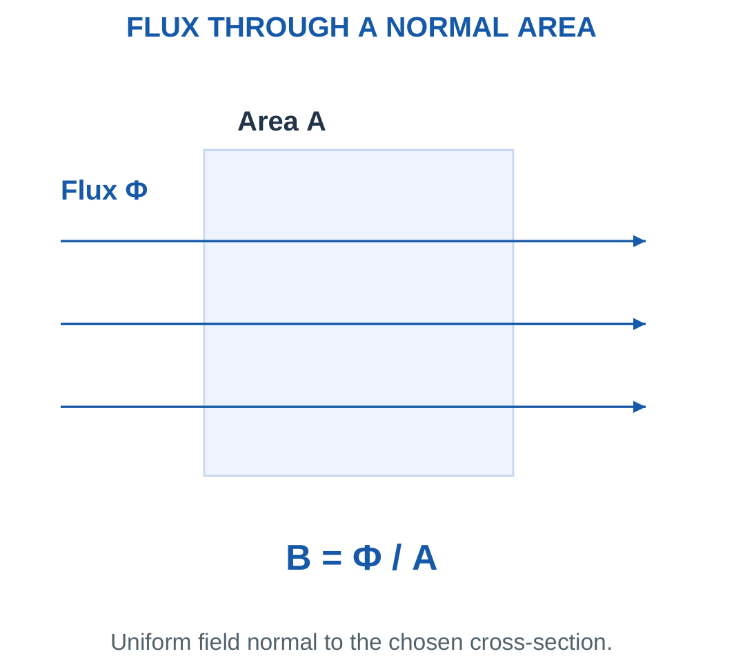
If a uniform field makes angle θ with the surface normal:
Φ = BA cos θ
The angle is measured from the normal rather than from the surface. If the angle is measured from the surface, the corresponding trigonometric relationship must be adjusted.
In a simple core model, the cross-sectional area is taken normal to the main flux path.
Flux and Flux Linkage
Flux through one turn is Φ. If all N turns link the same flux:
λ = NΦ
The quantity λ is flux linkage, conventionally expressed in Wb-turn.
Turn count multiplies flux linkage. It does not directly multiply flux density.
Faraday’s law concerns the rate of change of flux linkage. A winding can therefore have considerable steady linkage without having an induced EMF at that instant.
Area Conversions
1 cm² = 10⁻⁴ m²
1 mm² = 10⁻⁶ m²
A core area of 5 cm² is 0.0005 m². It is not 0.05 m².
Area conversion uses the square of a length conversion. An incorrect area factor changes calculated flux density by orders of magnitude.
Worked Problem 4.1: Flux Density and Winding Linkage
Problem: A core carries 1.2 mWb through an area of 6 cm². A 200-turn coil links all the flux. Find B, linkage and the flux density if area halves.
Convert the data:
Φ = 0.0012 Wb
A = 0.0006 m²
Flux density:
B = Φ/A = 0.0012/0.0006.
B = 2 T.
Linkage:
λ = NΦ = 200 × 0.0012.
λ = 0.24 Wb-turn.
If the same flux passes through half the area:
Bnew = Φ/(A/2).
Bnew = 4 T.
This is the result of the stated geometric calculation. Whether a particular material can operate at that density requires its material data.
Worked Problem 4.2: A Second Flux-Linkage Calculation
Problem: A core carries 0.8 mWb through 4 cm² and links a 500-turn winding.
Φ = 0.0008 Wb.
A = 0.0004 m².
B = 0.0008/0.0004.
B = 2 T.
λ = 500 × 0.0008.
λ = 0.4 Wb-turn.
At unchanged flux and half area:
Bnew = 4 T.
The same flux density as the previous example does not mean the same linkage. Linkage also depends on the number of turns and the total flux.
Worked Problem 4.3: Larger Flux and Area
Problem: A core carries 2.5 mWb through 10 cm². A 120-turn winding links the flux.
Φ = 0.0025 Wb.
A = 0.001 m².
B = 0.0025/0.001.
B = 2.5 T.
λ = 120 × 0.0025.
λ = 0.3 Wb-turn.
At half the original area and unchanged flux:
Bnew = 5 T.
The mathematical increase follows from B = Φ/A. A practical magnetic model must separately account for saturation and the excitation needed to maintain that flux.
2. MMF, Field Strength and Permeability
A coil of N turns carrying current I produces magnetomotive force:
F = NI
The conventional unit is ampere-turn.
Magnetomotive force is magnetic excitation. Despite its name, it is not a mechanical force measured in newtons.
For a uniform closed magnetic path of mean length l, Ampère’s law gives:
Hl = NI
Therefore:
H = NI/l
Magnetic field strength H is measured in A/m.
For a linear material:
B = μH
where:
μ = μ0μr
For the engineering calculations here:
μ0 ≈ 4π × 10⁻⁷ H/m
Relative permeability μr is dimensionless.

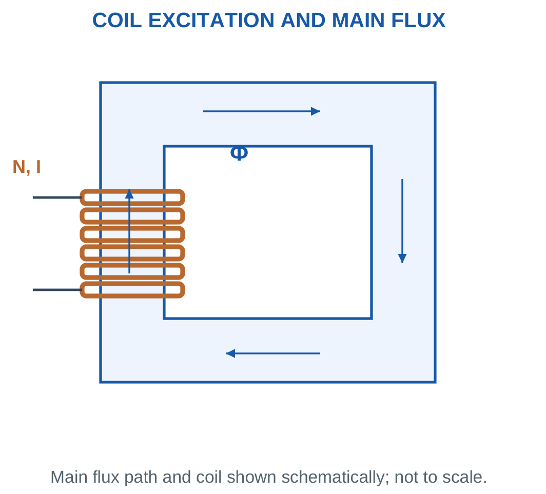
A larger permeability gives a larger B for the same H within the linear model.
Air has relative permeability approximately one. A magnetic core can have a much larger stated effective permeability.
Constant-Permeability Assumption
Ferromagnetic permeability is not constant over every operating condition.
Use a supplied constant μr only under the problem’s stated model. If a B–H characteristic is supplied, obtain H at the required B instead of imposing an unrelated constant permeability.
Current direction and winding sense determine flux direction. A numerical MMF magnitude alone does not define a unique flux arrow.
Worked Problem 4.4: MMF, H and B
Problem: A 400-turn coil carries 0.5 A on a uniform core of mean length 0.4 m and μr = 1000.
MMF:
F = 400 × 0.5.
F = 200 A-turn.
Field strength:
H = 200/0.4.
H = 500 A/m.
Permeability:
μ = 4π × 10⁻⁷ × 1000.
μ = 0.00125664 H/m.
Flux density:
B = μH.
B = 0.628319 T.
The calculation assumes the supplied permeability is applicable at the operating point.
Magnetic Excitation Hardware

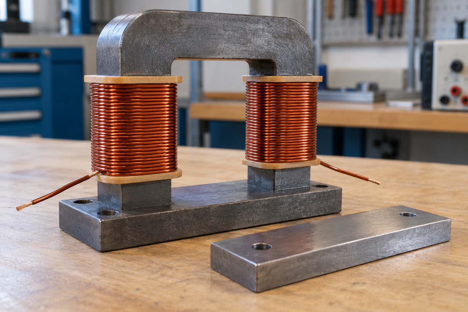
Current and turns provide excitation, but the resulting flux also depends on path length, area and material behaviour.
A winding-current value alone is therefore insufficient to determine flux without information about the magnetic circuit.
Worked Problem 4.5: Another Excitation Calculation
Problem: A 200-turn coil carries 1 A on a core of mean length 0.5 m and μr = 1200.
F = NI.
F = 200 A-turn.
H = 200/0.5.
H = 400 A/m.
μ = 4π × 10⁻⁷ × 1200.
μ = 0.00150796 H/m.
B = μH.
B = 0.603186 T.
Although the ampere-turns equal those of the preceding example, the different path length and permeability produce a different flux density.
3. Reluctance and the Magnetic-Circuit Equation
Reluctance describes opposition to establishing magnetic flux.
Its symbol is ℜ. For a uniform linear magnetic section:
ℜ = l/(μA)
Its unit is A-turn/Wb.
A longer path increases reluctance. A larger cross-sectional area or higher permeability reduces it.
Combining:
NI = Hl
B = μH
Φ = BA
gives:
Φ = NI/ℜ
This is the simple magnetic-circuit equation.

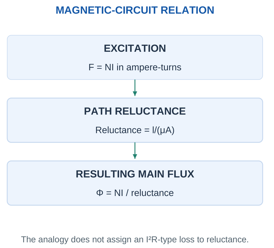
| Electrical Circuit | Magnetic-Circuit Analogy |
|---|---|
| EMF | MMF |
| Current | Flux |
| Resistance | Reluctance |
| I = V/R | Φ = NI/ℜ |
The analogy is useful for equations, but the physical processes differ.
Electrical resistance dissipates I²R watts. Reluctance is not an electrical resistor that dissipates Φ²ℜ watts.
Actual AC magnetic losses require hysteresis, eddy-current or other specified loss models.
Mean Path Length
The mean magnetic path follows the approximate centre of the core section.
It is not automatically the outer or inner perimeter. Use the mean length supplied in the problem or the stated geometric approximation.
Use a clear reluctance symbol so that magnetic reluctance is not confused with electrical winding resistance.
Worked Problem 4.6: Flux from Core Reluctance

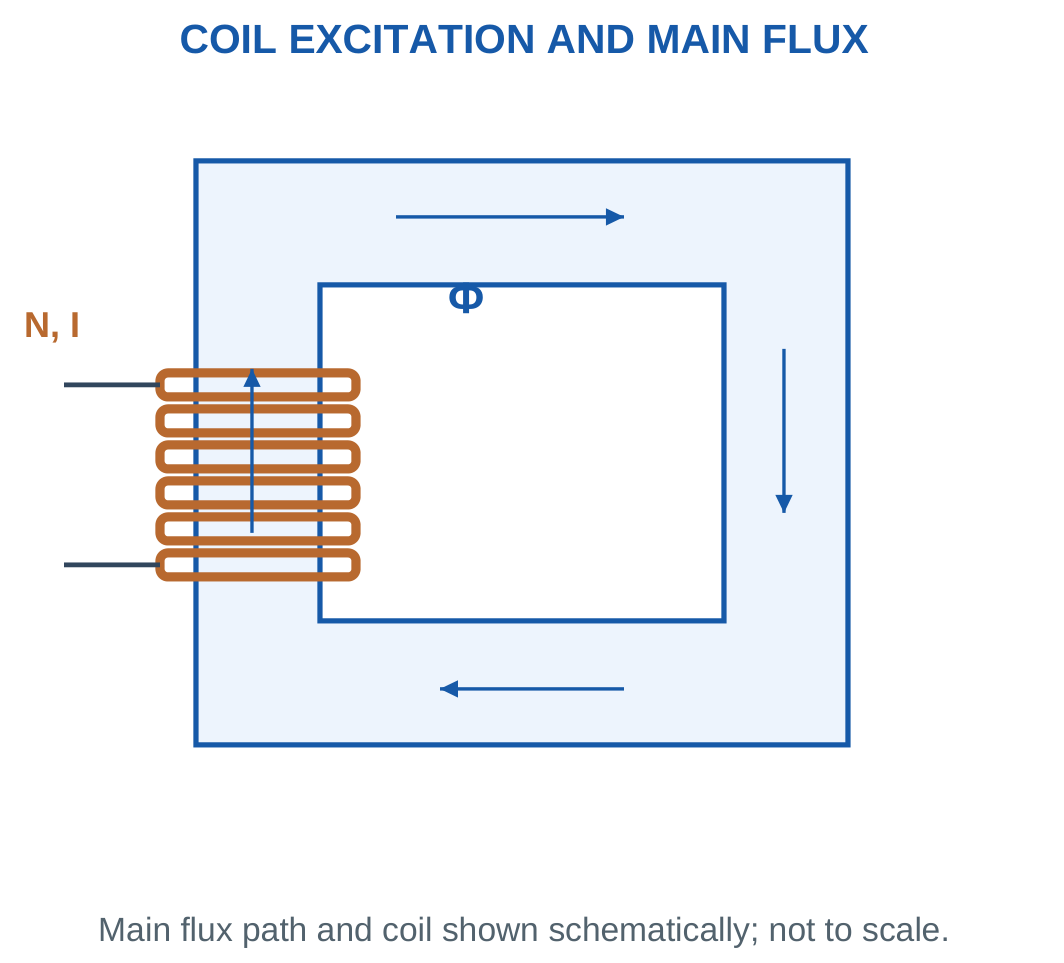
Problem: l = 0.4 m, A = 5 cm², μr = 1000, N = 500 and I = 0.4 A.
A = 0.0005 m².
μ = 0.00125664 H/m.
Reluctance:
ℜ = 0.4/(0.00125664 × 0.0005).
ℜ = 636,620 A-turn/Wb.
MMF:
NI = 200 A-turn.
Flux:
Φ = 200/636,620.
Φ = 0.314159 mWb.
Flux density:
B = 0.628319 T.
The independent calculation H = NI/l and B = μH gives the same result.
Worked Problem 4.7: A Different Linear Core
Problem: l = 0.3 m, A = 8 cm², μr = 1200, N = 300 and I = 0.5 A.
A = 0.0008 m².
μ = 0.00150796 H/m.
ℜ = 248,680 A-turn/Wb.
MMF:
NI = 150 A-turn.
Flux:
Φ = 0.603186 mWb.
Flux density:
B = 0.753982 T.
Here H = 150/0.3 = 500 A/m. Multiplication by the stated permeability confirms the same B.
Worked Problem 4.8: A Longer Core
Problem: l = 0.5 m, A = 10 cm², μr = 800, N = 600 and I = 0.25 A.
A = 0.001 m².
μ = 0.00100531 H/m.
ℜ = 497,359 A-turn/Wb.
MMF:
150 A-turn.
Flux:
Φ = 0.301593 mWb.
Flux density:
B = 0.301593 T.
The same MMF as the previous example gives less flux because the magnetic path has a different reluctance.
Worked Problem 4.9: A Shorter Core with Higher Permeability
Problem: l = 0.25 m, A = 4 cm², μr = 1500, N = 250 and I = 0.3 A.
A = 0.0004 m².
μ = 0.00188496 H/m.
ℜ = 331,573 A-turn/Wb.
MMF:
75 A-turn.
Flux:
Φ = 0.226195 mWb.
Flux density:
B = 0.565487 T.
Checking H = 75/0.25 = 300 A/m and B = μH verifies the result.
4. Simple Series Magnetic Circuits
In a series magnetic path with negligible leakage, the same main flux passes through every section.
The sections may have different lengths, areas and permeabilities.
For section k:
ℜk = lk/(μkAk)
Total reluctance is:
ℜtotal = ℜ1 + ℜ2 + …
The excitation requirement is:
NI = ΦΣℜ


A smaller-area section has larger B for the same flux.
Therefore flux continuity does not mean equal flux density in every section.
An alternative method is to calculate B in each section, obtain its H from the material model and add the MMF drops Hl.
For linear sections, this gives the same result as adding reluctances.
Calculation Procedure
Identify the main flux path. List each section’s length, area and permeability.
Convert units before forming reluctance.
If excitation is given, add reluctances and calculate flux. Then calculate B separately in each section.
If flux is given, calculate the required section MMFs and divide their sum by turns.
With several exciting coils, add or subtract their ampere-turns according to winding sense. Current magnitudes alone cannot be added without considering turn count and direction.
Worked Problem 4.10: Two-Section Magnetic Circuit

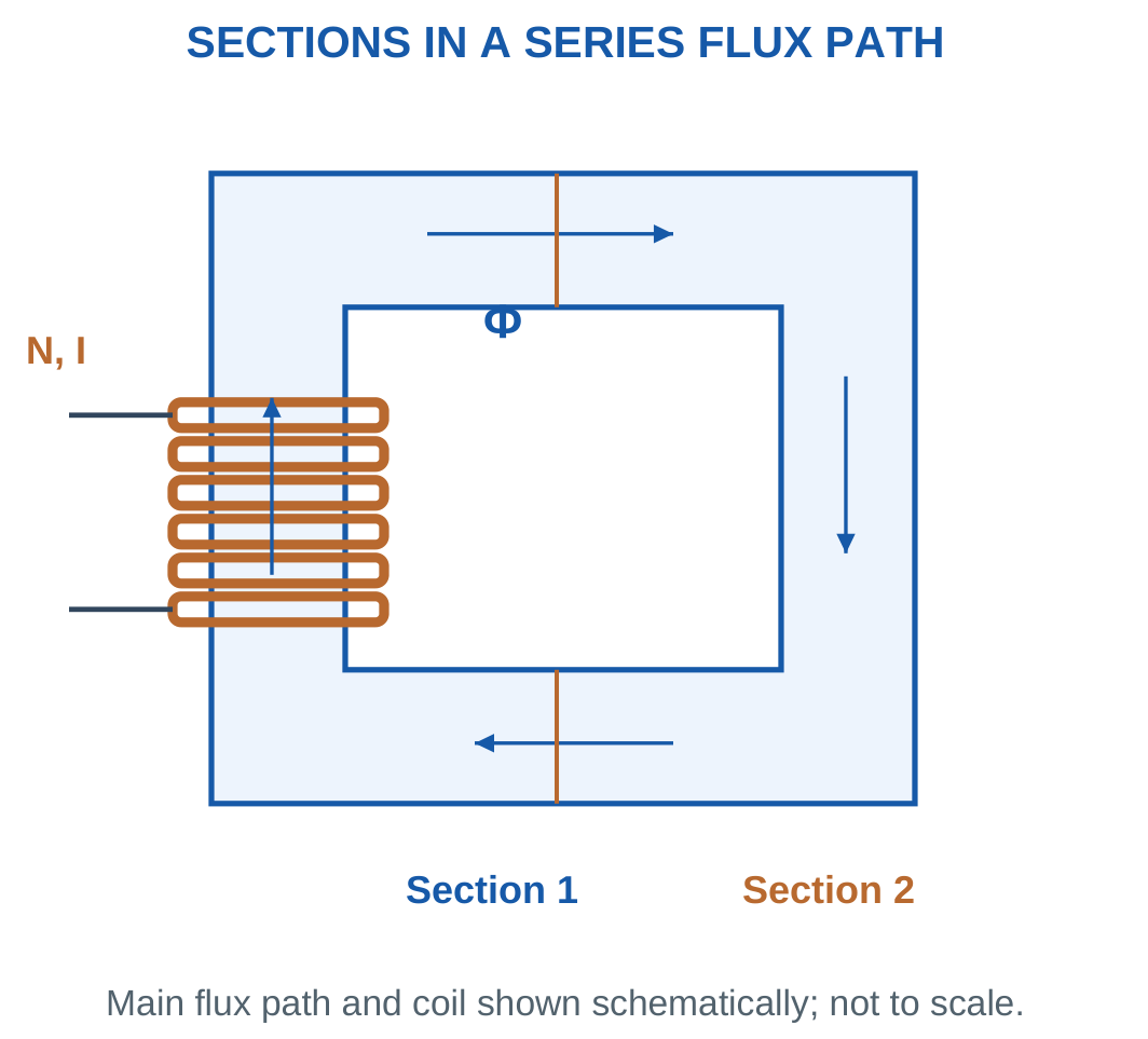
Problem: Section 1 has l = 0.2 m, A = 5 cm² and μr = 1000. Section 2 has l = 0.15 m, A = 4 cm² and μr = 800. Find current in 500 turns for 0.4 mWb.
Flux:
Φ = 0.0004 Wb.
Flux densities:
B1 = 0.8 T.
B2 = 1 T.
Reluctances:
ℜ1 = 318,310 A-turn/Wb.
ℜ2 = 373,019 A-turn/Wb.
MMF drops:
F1 = 127.324 A-turn.
F2 = 149.208 A-turn.
Total:
F = 276.532 A-turn.
Current:
I = F/N.
I = 0.553063 A.
Worked Problem 4.11: Second Two-Section Path
Problem: Section 1 has l = 0.25 m, A = 8 cm² and μr = 1200. Section 2 has l = 0.1 m, A = 6 cm² and μr = 900. Required flux is 0.6 mWb with 400 turns.
Flux densities:
B1 = 0.75 T.
B2 = 1 T.
Reluctances:
ℜ1 = 207,233 A-turn/Wb.
ℜ2 = 147,366 A-turn/Wb.
MMF drops:
124.34 A-turn and 88.4194 A-turn.
Total excitation:
212.759 A-turn.
Required current:
I = 0.531898 A.
The larger-area section has the smaller flux density even though both sections carry the same flux.
Worked Problem 4.12: Larger Series Core
Problem: Section 1 has l = 0.3 m, A = 10 cm² and μr = 1500. Section 2 has l = 0.2 m, A = 8 cm² and μr = 1000. Find current in 600 turns for 0.8 mWb.
Flux densities:
B1 = 0.8 T.
B2 = 1 T.
Reluctances:
159,155 and 198,944 A-turn/Wb.
MMF drops:
127.324 and 159.155 A-turn.
Total MMF:
286.479 A-turn.
Required current:
I = 0.477465 A.
Checking each section using H = B/μ and F = Hl confirms the same total.
Worked Problem 4.13: Unequal Areas and Materials
Problem: Section 1 has l = 0.12 m, A = 4 cm² and μr = 700. Section 2 has l = 0.18 m, A = 5 cm² and μr = 1100. Required flux is 0.3 mWb with 300 turns.
Flux densities:
B1 = 0.75 T.
B2 = 0.6 T.
Reluctances:
341,046 and 260,435 A-turn/Wb.
MMF drops:
102.314 and 78.1306 A-turn.
Total:
180.445 A-turn.
Current:
I = 0.601482 A.
The two material sections require different field strengths and MMF drops. They are not assigned a common H merely because flux is common.
5. Series Air Gap and Its Effect
An air gap has much lower permeability than a typical magnetic core.
Its reluctance is:
ℜgap = g/(μ0Agap)
Even a short gap can contribute a substantial fraction of total reluctance.
For a series core and gap:
ℜtotal = ℜcore + ℜgap

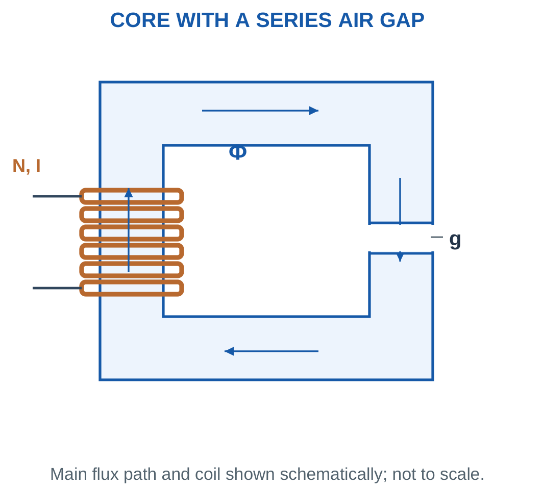
For a specified gap flux density:
Fgap = Hgapg = Bg/μ0
Core MMF must still be included unless the problem explicitly permits it to be neglected.
If effective gap area differs from core area, calculate the corresponding flux densities separately.
Assumptions for Gap Problems
The following calculations neglect leakage and fringing unless an effective gap area is supplied.
Core length means magnetic-material length. The air-gap length is a separate section and must not be counted twice.
Fringing is flux spreading near the gap faces. It can increase effective gap area. A numerical correction requires a supplied model rather than an invented percentage.
At fixed NI, adding a gap reduces flux in the linear model.
At fixed required flux, adding a gap increases required ampere-turns.
Worked Problem 4.14: Required Current with an Air Gap

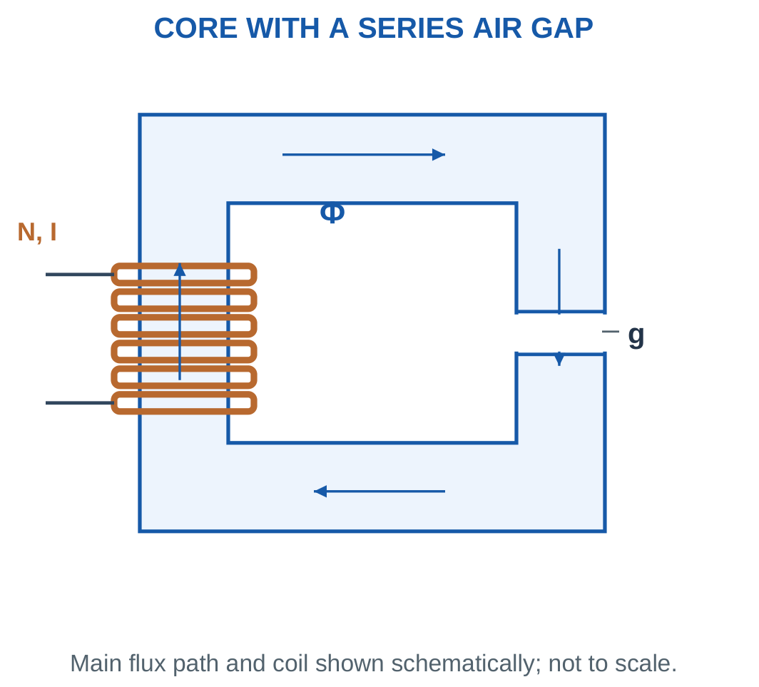
Problem: Core length is 0.4 m, area is 5 cm² and μr = 1000. Gap length is 0.5 mm. A 500-turn coil must produce B = 0.8 T.
Area:
A = 0.0005 m².
Gap:
g = 0.0005 m.
Flux:
Φ = BA.
Φ = 0.0004 Wb.
Core reluctance:
636,620 A-turn/Wb.
Gap reluctance:
795,775 A-turn/Wb.
Core MMF:
254.648 A-turn.
Gap MMF:
318.31 A-turn.
Total excitation:
572.958 A-turn.
Current:
I = 1.14592 A.
Core with a Defined Air Gap


The illustration shows the geometric idea. Numerical dimensions and material assumptions come from the problem.
A gap can dominate reluctance without being physically long because its permeability differs greatly from that of the core.
Worked Problem 4.15: Another Gapped Core
Problem: Core length is 0.5 m, area is 10 cm² and μr = 800. Gap is 0.25 mm. Find current in 400 turns for B = 0.9 T.
Flux:
Φ = 0.9 × 0.001.
Φ = 0.0009 Wb.
Core reluctance:
497,359 A-turn/Wb.
Gap reluctance:
198,944 A-turn/Wb.
Core MMF:
447.623 A-turn.
Gap MMF:
179.049 A-turn.
Total:
626.673 A-turn.
Current:
I = 1.56668 A.
Here the core contribution is greater than the gap contribution. The existence of an air gap does not justify neglecting the core automatically.
Worked Problem 4.16: Gap-Dominated Reluctance
Problem: Core length is 0.25 m, area is 4 cm² and μr = 1200. Gap is 0.75 mm. A winding of 800 turns must produce B = 0.7 T.
Required flux:
0.00028 Wb.
Core reluctance:
414,466 A-turn/Wb.
Gap reluctance:
1.49208 × 10⁶ A-turn/Wb.
The gap/core reluctance ratio is 3.6.
Core MMF:
116.05 A-turn.
Gap MMF:
417.782 A-turn.
Total:
533.832 A-turn.
Current:
I = 0.66729 A.
The gap dominates but the core MMF remains part of the requested complete calculation.
6. B–H Behaviour, Saturation and Model Limits
Ferromagnetic materials do not maintain one constant relationship between B and H over all operating points.
At higher excitation, the B–H curve bends. Increasing H then produces a smaller incremental increase in B.
This behaviour is called saturation.

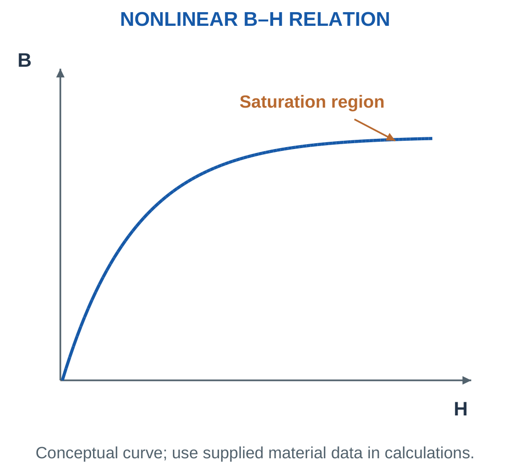
If material data are supplied, calculate B = Φ/A for each section and obtain the corresponding H from the data.
Then calculate MMF as Hl.
Use interpolation only within the supplied range and according to the stated assumptions.
Saturation and Hysteresis
Saturation concerns the excitation–flux relationship.
Hysteresis concerns the dependence of magnetic state on previous magnetisation. In AC operation, the area of a B–H loop represents energy dissipated per unit volume per cycle.
These are related aspects of material behaviour, but they are not the same phenomenon.
Reluctance alone is not a complete core-loss model. Hysteresis and eddy-current losses are represented separately in practical transformer analysis.
Worked Problem 4.17: Use a Supplied B–H Point
Problem: A material table gives H = 350 A/m at B = 0.8 T. Core length is 0.4 m, area is 5 cm² and turns are 500.
Area:
0.0005 m².
Flux:
Φ = BA.
Φ = 0.0004 Wb.
MMF:
F = Hl = 350 × 0.4.
F = 140 A-turn.
Current:
I = 140/500.
I = 0.28 A.
The operating-point ratio B/H is 0.00228571 H/m. It does not establish that permeability or differential slope remains constant at another point.
Worked Problem 4.18: A Second Material Point
Problem: A table gives H = 700 A/m at B = 1.1 T. Core length is 0.3 m, area is 8 cm² and turns are 600.
Flux:
Φ = 1.1 × 0.0008.
Φ = 0.00088 Wb.
MMF:
F = 700 × 0.3.
F = 210 A-turn.
Current:
I = 210/600.
I = 0.35 A.
No additional permeability factor is inserted because H is already supplied for the required operating flux density.
Laminated Magnetic Core

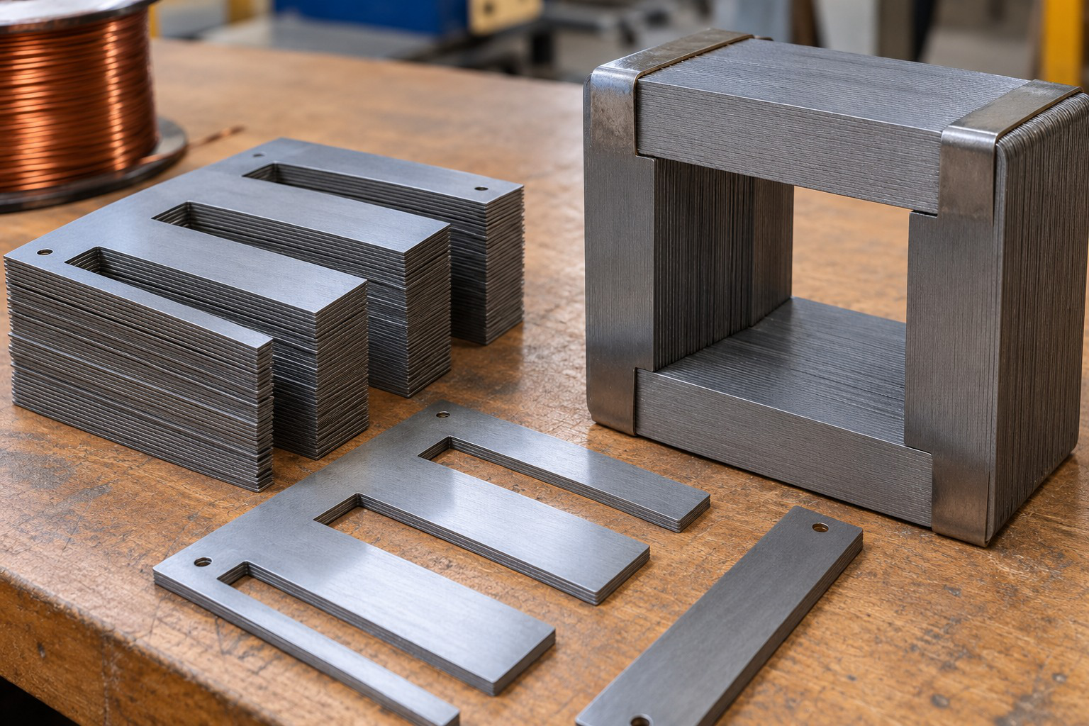
Lamination is a construction feature used in many AC magnetic cores. It reduces large circulating eddy-current paths.
A visible stack does not independently establish a numerical permeability, core-loss value or permissible flux density.
7. Faraday’s Law and Lenz’s Law
A changing flux linkage induces an EMF.
Faraday’s law is:
e = −dλ/dt
If N fixed turns link the same flux:
e = −N dΦ/dt
For a uniform finite flux change:
eavg = −NΔΦ/Δt

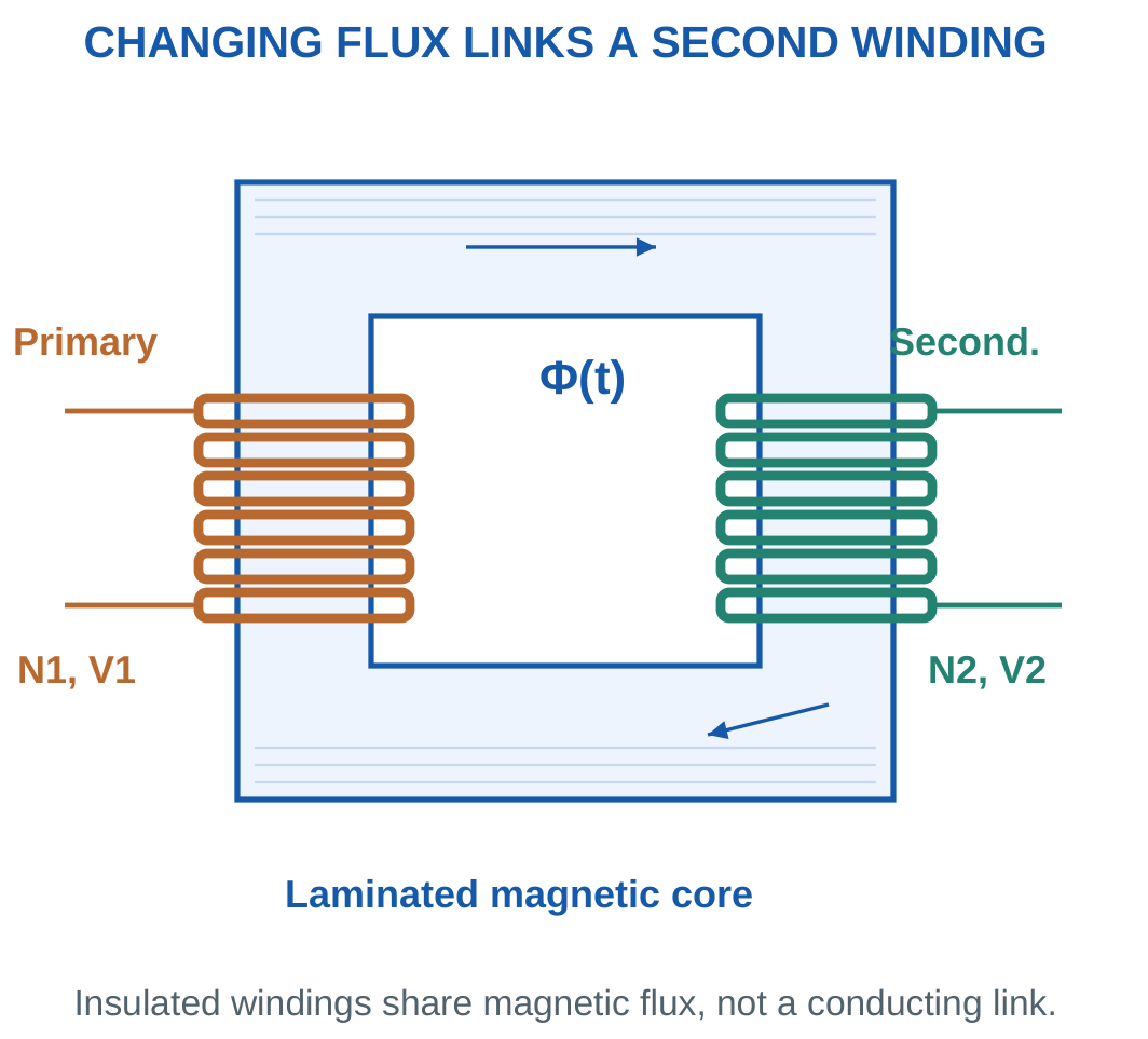
Lenz’s law explains the minus sign. The induced effect opposes the change producing it.
It does not mean that a numerical voltage must be negative for every possible terminal reference.
A stationary winding can have induced EMF when the linked magnetic field changes. Mechanical motion is one way of changing linkage, but it is not necessary for transformer induction.
Use the Full Flux Change
For a finite interval:
ΔΦ = Φfinal − Φinitial
A reversal from +2 mWb to −2 mWb gives a change of −4 mWb.
Steady nonzero flux gives zero induced EMF in a stationary fixed-turn coil because its derivative is zero.
For nonuniform variation, ΔΦ/Δt gives average EMF. Instantaneous EMF requires the actual derivative of the stated flux function.
Worked Problem 4.19: Average Induced EMF

Problem: A 200-turn coil has flux per turn changing uniformly from 1 mWb to 3 mWb in 20 ms.
ΔΦ = 0.003 − 0.001.
ΔΦ = 0.002 Wb.
Δt = 0.02 s.
Rate:
0.1 Wb/s.
e = −200 × 0.1.
e = −20 V.
Magnitude is 20 V. The uniform-slope assumption makes this value constant within the interior of the stated interval.
Worked Problem 4.20: Flux Reversal
Problem: A 500-turn coil has flux changing from +2 mWb to −2 mWb in 10 ms.
ΔΦ = −0.002 − 0.002.
ΔΦ = −0.004 Wb.
Δt = 0.01 s.
Rate:
−0.4 Wb/s.
e = −500 × (−0.4).
e = +200 V.
Using only the final flux magnitude would miss the complete reversal and produce an incorrect result.
Worked Problem 4.21: Flux Falling to Zero
Problem: A 100-turn coil has flux changing from 0.5 mWb to zero in 5 ms.
ΔΦ = −0.0005 Wb.
Δt = 0.005 s.
Rate:
−0.1 Wb/s.
e = −100 × (−0.1).
e = +10 V.
The sign belongs to the declared linkage and induced-EMF reference. Its magnitude is 10 V.
Worked Problem 4.22: Negative to Positive Flux
Problem: A 300-turn coil has flux changing from −1 mWb to +2 mWb in 15 ms.
ΔΦ = 0.002 − (−0.001).
ΔΦ = 0.003 Wb.
Δt = 0.015 s.
Rate:
0.2 Wb/s.
e = −300 × 0.2.
e = −60 V.
A signed change must be calculated before applying the negative derivative convention.
8. Sinusoidal Flux and Induced Voltage
Let the flux be:
Φ(t) = Φm sin ωt
Here Φm is peak flux.
Differentiating:
dΦ/dt = ωΦm cos ωt
Therefore:
e = −NωΦm cos ωt
Induced EMF magnitude is greatest at flux zero crossings and zero at flux maxima and minima.

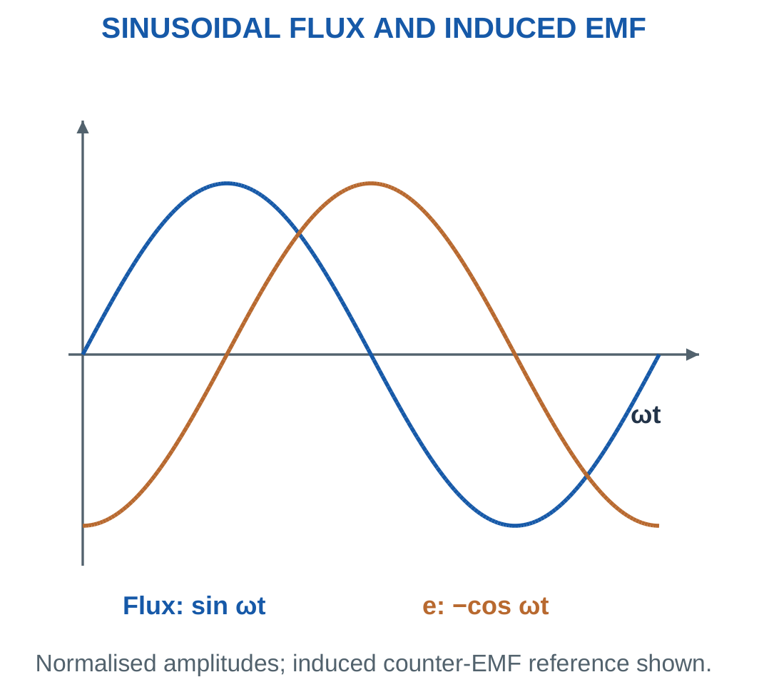
Peak EMF magnitude is:
Em = 2πfNΦm
RMS magnitude is:
E = Em/√2
Therefore:
E = √2πfNΦm ≈ 4.44fNΦm
The positive RMS expression gives magnitude, not the complete signed terminal-polarity relationship.
Applied winding voltage approximately balances induced counter-EMF when winding drops are neglected.
Peak Flux and Waveform Shape
Use peak flux in the EMF equation.
If RMS flux is supplied for a sinusoid, first obtain its peak.
The 4.44 coefficient follows from sinusoidal flux. It is not a universal coefficient for every waveform shape.
The exact coefficient √2π is approximately 4.44288. Small differences from 4.44 calculations are coefficient-rounding differences.
Worked Problem 4.23: Sinusoidal Flux at a Zero Crossing
Problem: Φ = 1 mWb sin(2π × 50t) in a 200-turn winding. Find peak EMF, exact RMS EMF and e at flux angle zero.
Peak flux:
0.001 Wb.
Angular frequency:
314.159 rad/s.
Peak EMF:
Em = NωΦm.
Em = 62.8319 V.
Exact sinusoidal RMS:
E = 44.4288 V.
The conventional 4.44 equation gives 44.4 V.
At flux angle zero:
e = −Em cos 0°.
e = −62.8319 V.
Flux is zero but its rate of change is maximum.
Worked Problem 4.24: Sinusoidal Flux at Its Peak
Problem: Φ = 0.8 mWb sin(2π × 60t) in a 500-turn winding. Evaluate e at flux angle 90°.
Φm = 0.0008 Wb.
ω = 376.991 rad/s.
Em = 150.796 V.
Exact RMS EMF:
106.629 V.
Using 4.44 gives 106.56 V.
At 90°:
e = −Em cos 90°.
e = 0 V.
At a flux maximum the slope is zero. A large instantaneous flux is therefore compatible with zero instantaneous induced EMF.
Worked Problem 4.25: Sinusoidal Flux at 30°
Problem: Φ = 2 mWb sin(2π × 25t) in a 100-turn coil.
Φm = 0.002 Wb.
ω = 157.08 rad/s.
Em = 31.4159 V.
Exact RMS:
22.2144 V.
Conventional RMS:
22.2 V.
At flux angle 30°:
e = −31.4159 cos 30°.
e = −27.207 V.
The numerical sign reflects the selected induced-EMF reference, while the RMS magnitude remains positive.
9. Self-Inductance and Flux Linkage
Self-inductance describes the linkage of a coil’s own magnetic field with its turns.
For a linear magnetic circuit:
L = λ/I = NΦ/I
The unit is the henry.
Using Φ = NI/ℜ:
L = N²/ℜ


With unchanged reluctance, doubling turns multiplies inductance by four.
The current-turn excitation contributes one turn factor. Flux linkage contributes another.
A larger reluctance reduces inductance. Introducing an air gap generally lowers L for the same winding under the stated linear model.
Linear and Nonlinear Inductance
For a linear constant-L model, linkage and current are proportional.
With nonlinear magnetic behaviour, the ratio λ/i and the slope dλ/di need not be equal.
Do not apply a constant-inductance model through saturation without the required assumptions.
A steady current can maintain stored magnetic energy even when induced EMF is zero. EMF depends on changing linkage rather than its mere existence.
Inductor Winding

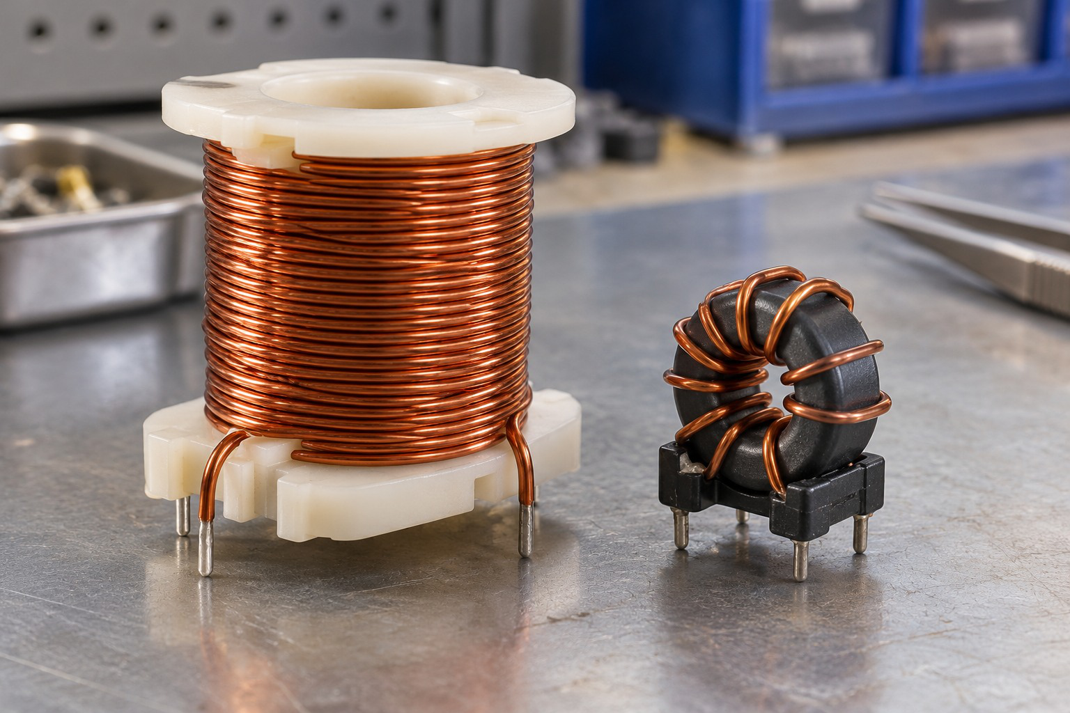
Real windings can include electrical resistance and core effects. Their practical behaviour differs from a loss-free constant inductance when those effects are significant.
The numerical problem determines which model is appropriate.
Worked Problem 4.26: Inductance from Flux Linkage
Problem: A 200-turn linear coil carries 2 A and links 0.8 mWb per turn.
Linkage:
λ = 200 × 0.0008.
λ = 0.16 Wb-turn.
Inductance:
L = λ/I.
L = 0.08 H.
Reluctance:
ℜ = NI/Φ.
ℜ = 500,000 A-turn/Wb.
Checking N²/ℜ gives 0.08 H.
If turns double with reluctance unchanged:
Lnew = 0.32 H.
The flux also changes at unchanged current in this linear model.
Worked Problem 4.27: A Higher-Turn Coil
Problem: An 800-turn coil carries 0.4 A and links 0.6 mWb per turn.
Linkage:
λ = 800 × 0.0006.
λ = 0.48 Wb-turn.
L = 0.48/0.4.
L = 1.2 H.
Reluctance:
533,333 A-turn/Wb.
After doubling turns:
Lnew = 4.8 H.
The fourfold change assumes that geometry and permeability remain represented by the same reluctance.
10. Self-Induced EMF and Stored Energy
For constant inductance, the referenced counter-EMF is:
e = −L di/dt
With passive terminal polarity, the ideal inductor voltage is:
vL = L di/dt
These signs use different references. They should not be mixed within one KVL equation.

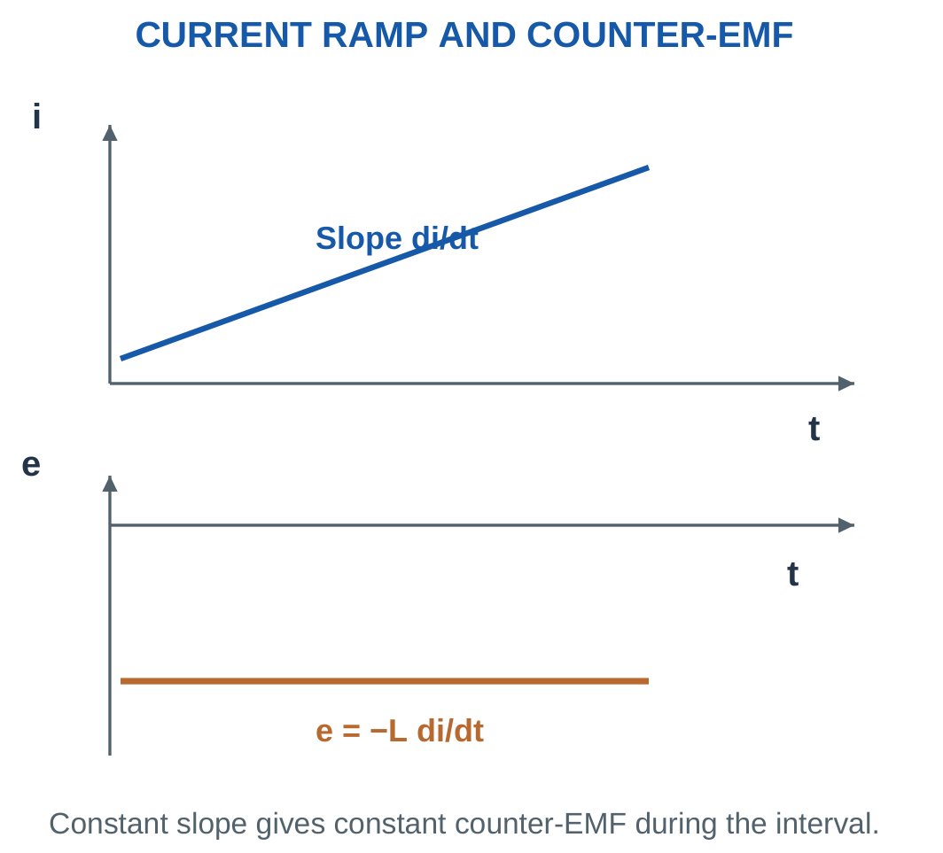
For a uniform current change, induced-EMF magnitude is:
|e| = L|ΔI|/Δt
Stored magnetic energy in a linear inductor is:
Wm = LI²/2
The current is the instantaneous current relevant to the requested energy.
Maximum sinusoidal energy uses peak current. A stated DC steady current is used directly.
Stored Energy Is Not Automatically Loss
An ideal field can return stored energy to the circuit.
It should not automatically be counted as copper heat or core loss.
For nonlinear behaviour, stored energy requires the appropriate linkage-current integral rather than an unqualified LI²/2 expression.
Worked Problem 4.28: Current Ramp from Zero
Problem: A 0.2 H inductor current rises uniformly from zero to 3 A in 10 ms.
Rate:
di/dt = 3/0.01.
di/dt = 300 A/s.
Counter-EMF:
e = −0.2 × 300.
e = −60 V.
Initial energy:
W1 = 0 J.
Final energy:
W2 = 0.2 × 3²/2.
W2 = 0.9 J.
Energy increase is 0.9 J. The corresponding passive terminal voltage has the opposite reference sign to the counter-EMF used here.
Solenoid and Moving Plunger


Magnetic fields can produce force and motion. In real devices, inductance may vary with mechanical position.
A simple constant-geometry magnetic calculation must state the assumptions under which its reluctance and inductance remain fixed.
Worked Problem 4.29: Current Reversal with Equal Endpoint Energy
Problem: A 0.4 H inductor current changes from −2 A to +2 A in 20 ms.
Current change:
ΔI = 4 A.
Rate:
200 A/s.
Counter-EMF:
e = −0.4 × 200.
e = −80 V.
Initial energy:
0.4 × (−2)²/2.
W1 = 0.8 J.
Final energy:
0.4 × 2²/2.
W2 = 0.8 J.
Net change is zero, but energy is released as current approaches zero and stored again as its positive magnitude rises.
11. Mutual Inductance and Coupling
Changing current in one coil can change the flux linked by a second coil. The second coil then has mutually induced EMF.
For linear coupling:
|e2| = M|di1/dt|
Mutual inductance M is measured in henries.


If Φ21 is flux per secondary turn caused by primary current:
M = N2Φ21/I1
Flux that does not link the other winding is leakage flux and does not contribute to its mutual linkage.
For reciprocal linear coils:
M = k√(L1L2)
When M is quoted as a positive magnitude:
0 ≤ k ≤ 1
Perfect coupling has k = 1.
Physical Bound and Polarity
A mutual-inductance magnitude greater than √(L1L2) is inconsistent with the passive linear model.
Check the units before reporting a coupling coefficient above one.
The magnitude M does not by itself determine secondary terminal sign. Winding sense, dots and current references are also required.
Worked Problem 4.30: Coupling and Secondary EMF
Problem: L1 = 0.4 H, L2 = 0.1 H, k = 0.8 and primary current changes at 200 A/s.
Maximum mutual-inductance magnitude:
√(0.4 × 0.1).
0.2 H.
Actual mutual inductance:
M = 0.8 × 0.2.
M = 0.16 H.
Secondary EMF magnitude:
0.16 × 200.
|e2| = 32 V.
If primary current becomes constant, this mutually induced EMF becomes zero even though linked steady flux can remain.
Worked Problem 4.31: Higher Current-Change Rate
Problem: L1 = 0.2 H, L2 = 0.05 H, k = 0.9 and di1/dt = 500 A/s.
√(L1L2) = 0.1 H.
M = 0.9 × 0.1.
M = 0.09 H.
Secondary EMF magnitude:
45 V.
The result depends on current-change rate rather than the absolute current alone.
A larger steady primary current does not imply a larger induced secondary EMF if its rate of change is zero.
Worked Problem 4.32: Perfect Coupling
Problem: L1 = 0.6 H, L2 = 0.15 H, k = 1 and di1/dt = 100 A/s.
M = √(0.6 × 0.15).
M = 0.3 H.
Secondary induced-EMF magnitude:
0.3 × 100.
|e2| = 30 V.
The mutual inductance equals the passive upper bound because coupling is perfect in the stated model.
12. Mutual-Induction Calculations and Polarity
For a uniform primary-current change:
|e2| = M|ΔI1|/Δt
If current is constant, the induced voltage due to that current is zero during the constant interval.
The magnetic linkage can still be nonzero.


With voltages measured from dotted to undotted terminals and both currents entering dots, passive coupled-coil voltage equations contain positive mutual derivative terms.
Reversing one current reference changes the sign of its mutual contribution.
Most introductory problems ask for induced-EMF magnitude. Give a signed answer only when terminal and winding references are sufficient.
Mutual Induction and Electrical Isolation
Two insulated windings need not have a direct conducting connection to exchange energy through a changing field.
An ideal transformer is a special coupled-coil model with common linked flux and negligible losses.
Arbitrary loosely coupled coils do not automatically satisfy every ideal-transformer relation.
Worked Problem 4.33: M from Linked Secondary Flux
Problem: Primary current 2 A produces 0.2 mWb per turn linking a 300-turn secondary. Find M and EMF magnitude when primary current changes by 3 A in 10 ms.
Secondary linkage:
λ21 = 300 × 0.0002.
λ21 = 0.06 Wb-turn.
M = λ21/I1.
M = 0.03 H.
Current-change rate:
3/0.01.
300 A/s.
Induced secondary EMF magnitude:
9 V.
Its sign requires winding and voltage references beyond the magnitude data.
Transformer Winding and Insulation

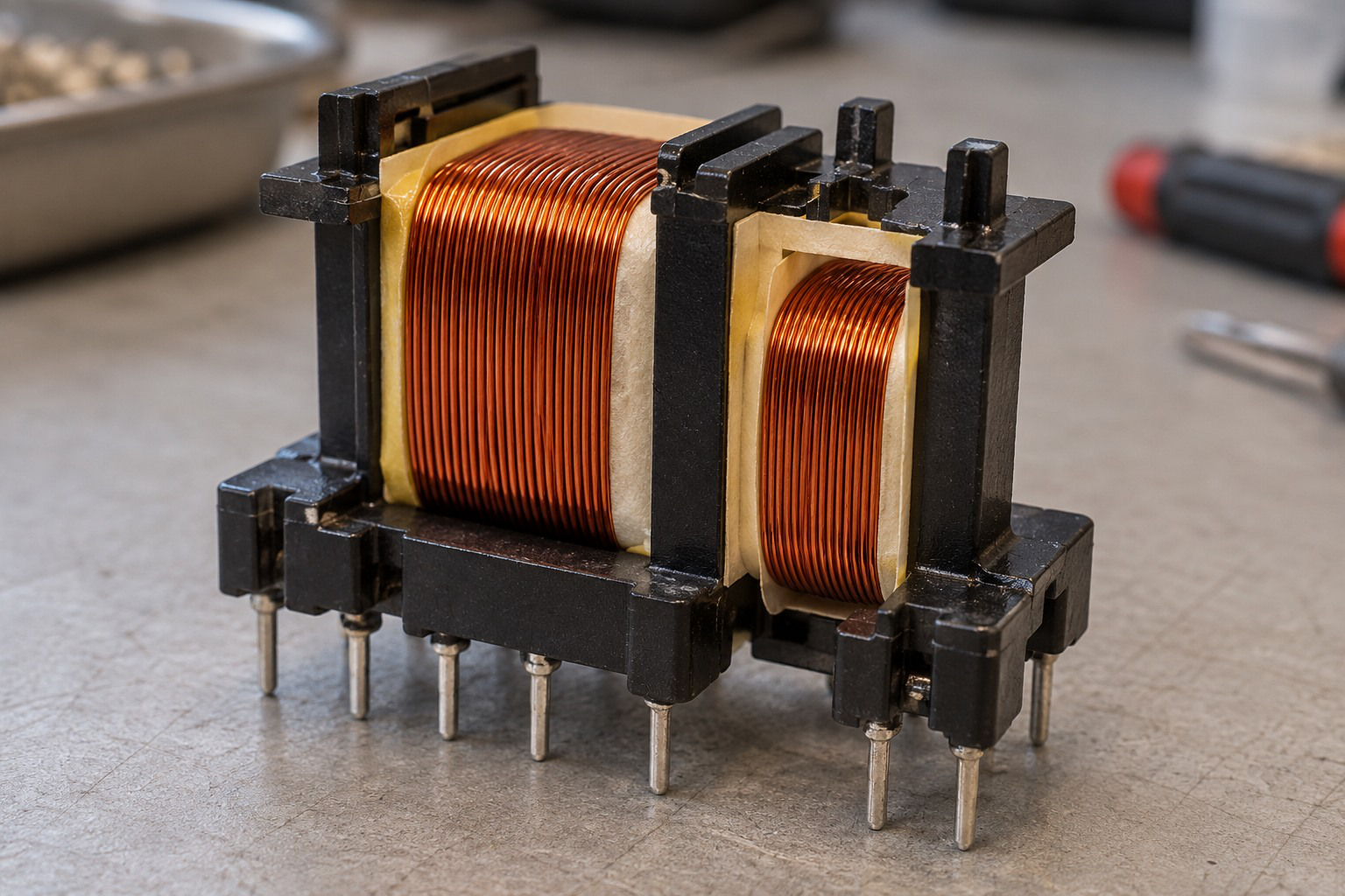
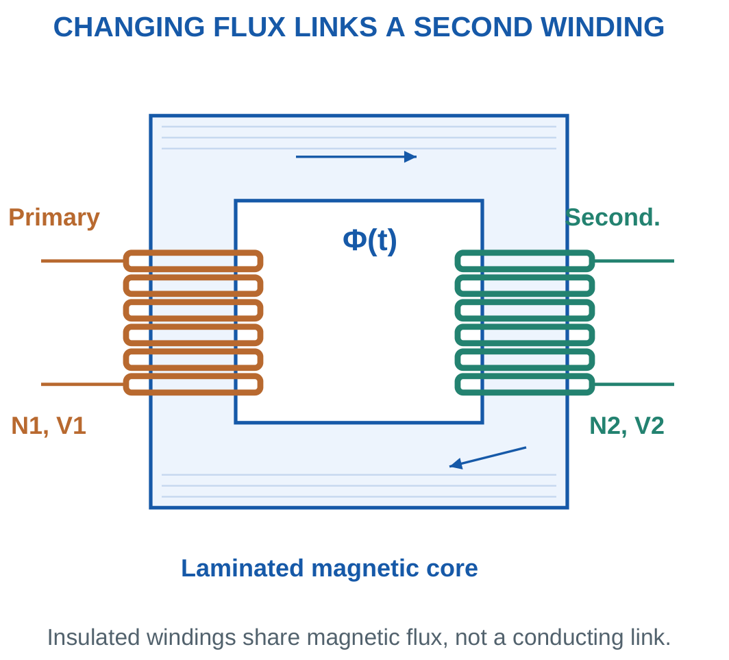
Windings share magnetic flux while insulation separates electrical paths.
Turns, conductor cross-section and insulation serve different requirements. A photograph does not independently provide a turn count, winding resistance or power rating.
Worked Problem 4.34: Another Linked-Flux Calculation
Problem: Primary current 4 A produces 0.4 mWb per secondary turn. The secondary has 200 turns. Current changes by 1 A in 20 ms.
Linkage:
λ21 = 200 × 0.0004.
λ21 = 0.08 Wb-turn.
M = 0.08/4.
M = 0.02 H.
Current-change rate:
1/0.02.
50 A/s.
Induced EMF magnitude:
1 V.
The current used in M = λ21/I1 is the primary current producing that linkage, not a secondary load current.
13. Single-Phase Transformer Construction
A transformer is a static electromagnetic device with windings linked by common alternating magnetic flux.
The primary is the winding connected to the input source in the selected use.
The secondary supplies the output load.
Either winding can have the greater turn count.


A magnetic core provides a low-reluctance path.
Insulation separates turns, windings and core.
Laminated cores use insulated sheets to reduce large eddy-current loops while retaining the required magnetic path.
Core-type and shell-type arrangements differ geometrically, but both use the same induction principle.
Two-Winding Isolation
A conventional two-winding transformer has no intended metallic connection between primary and secondary.
This statement does not apply to an autotransformer with a shared winding section.
Ordinary steady-state transformation preserves frequency. The transformer changes voltage and current levels according to turns.
Additional rectifiers or switching stages in a larger power product are separate from the basic transformer model.
Worked Problem 4.35: Step-Down Action
Problem: N1 = 1000 turns, N2 = 100 turns and V1 = 230 V RMS.
Define:
a = N1/N2.
a = 10.
Secondary voltage:
V2 = V1/a.
V2 = 23 V RMS.
The selected operating direction is step-down.
Both windings have the same frequency. Reversing input and output roles reverses the voltage ratio, subject to the model and winding ratings.
Low-Voltage Transformer


Shared changing flux links the windings. Turns ratio and load conditions determine the electrical quantities in the selected model.
The illustration provides physical context for the ideal transformer symbol and magnetic linkage.
Worked Problem 4.36: Equal-Voltage Transformation
Problem: N1 = 500 turns, N2 = 500 turns and input voltage is 240 V RMS.
a = 500/500.
a = 1.
V2 = 240/1.
V2 = 240 V RMS.
This is equal-voltage transformation.
Separate windings can provide electrical isolation even when voltage magnitude is unchanged. Isolation does not require a step-up or step-down ratio.
14. Operation at No Load and with a Load
An AC primary voltage establishes alternating flux.
Changing common flux induces EMF in both windings.
The primary induced counter-EMF balances most of the applied voltage when winding drops are small.

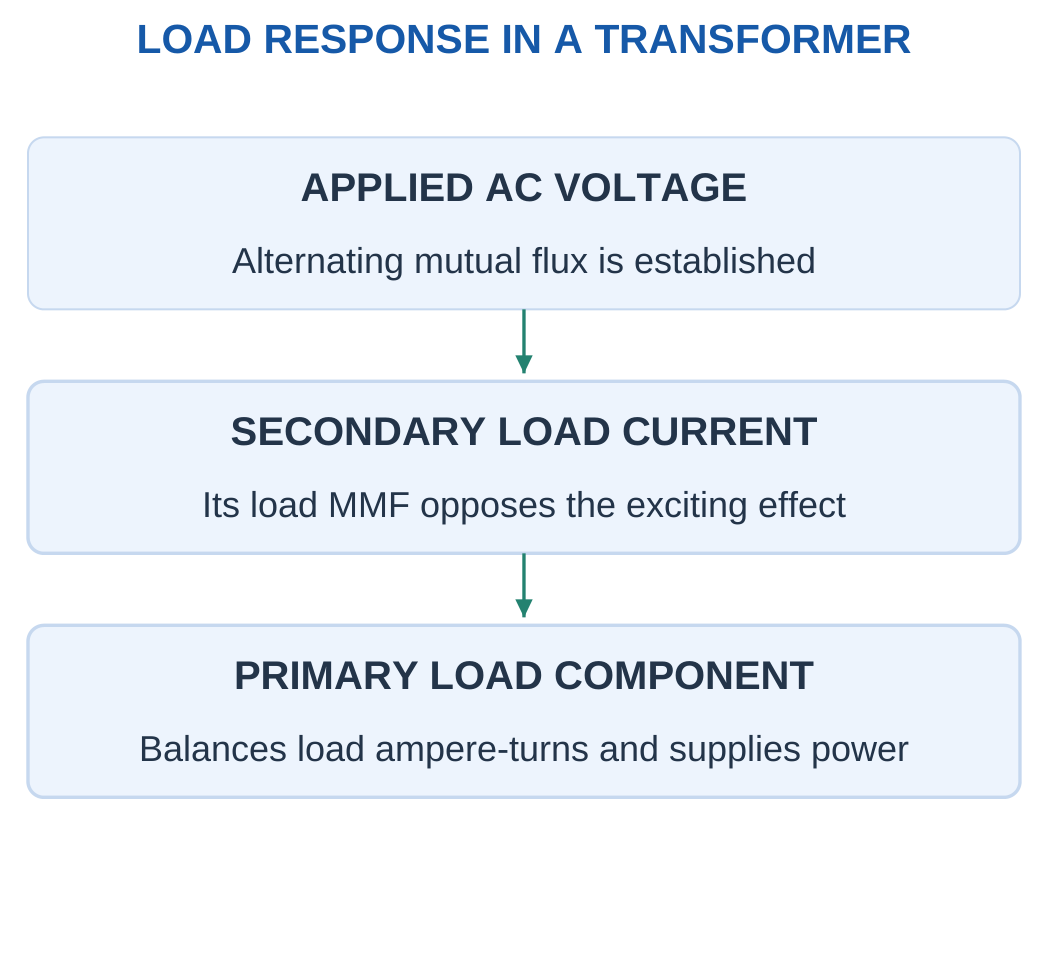
With an open secondary, a practical transformer still draws no-load current.
Its magnetising component establishes flux. Its active component supplies core loss.
The exact ideal model neglects these effects and can have zero no-load current.
When the secondary carries load current, its ampere-turns oppose the original flux-producing effect.
The primary draws an additional load-current component whose ampere-turns approximately balance the secondary load ampere-turns.
The main flux remains primarily set by applied voltage per frequency and primary turns under the normal low-drop model.
EMF and Terminal Voltage
Do not explain loading as simply destroying flux and ending induction.
The supply response provides additional primary current.
Practical winding drops cause terminal-voltage changes. Therefore distinguish internal induced EMFs E1 and E2 from terminal voltages V1 and V2.
Worked Problem 4.37: Load Ampere-Turn Balance
Problem: N1 = 1000, N2 = 200 and secondary current is 5 A.
a = 1000/200.
a = 5.
Primary load-current magnitude:
I1 = I2/a.
I1 = 1 A.
Primary load ampere-turns:
N1I1 = 1000 A-turn.
Secondary load ampere-turns:
N2I2 = 1000 A-turn.
They oppose in the ideal load balance. A practical excitation component is added phasorially to the primary load component.
Worked Problem 4.38: An 8:1 Turns Ratio
Problem: N1 = 800, N2 = 100 and I2 = 8 A.
a = 8.
I1 = 8/8.
I1 = 1 A.
Primary ampere-turn magnitude:
800 A-turn.
Secondary ampere-turn magnitude:
800 A-turn.
The voltage and current ratios are inverse. A larger primary turn count does not imply a larger primary load current for the same ideal transferred VA.
Worked Problem 4.39: Step-Up Current Relationship
Problem: N1 = 200, N2 = 600 and I2 = 2 A.
a = 200/600.
a = 1/3.
I1 = I2/a.
I1 = 6 A.
Primary ampere-turns:
200 × 6.
1200 A-turn.
Secondary ampere-turns:
600 × 2.
1200 A-turn.
The higher-voltage secondary carries less current in the ideal power-transfer model.
15. Transformer EMF Equation
Assume sinusoidal common core flux with peak Φm.
Faraday’s law gives peak induced-EMF magnitude:
Em = 2πfNΦm
For a sinusoidal voltage:
E = Em/√2
Therefore:
E = √2πfNΦm
Using the conventional coefficient:
E = 4.44fNΦm

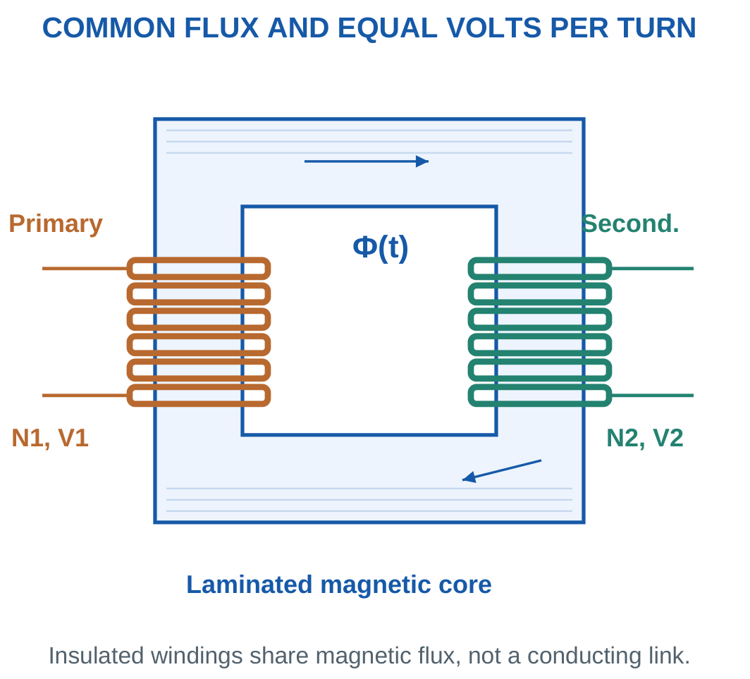
For the windings:
E1 = 4.44fN1Φm
E2 = 4.44fN2Φm
Thus:
E1/E2 = N1/N2
Both windings have equal RMS volts per turn:
Et = 4.44fΦm
With peak flux density and effective core area:
Φm = BmA
Therefore:
E = 4.44fNBmA
Use the net effective area supplied. Do not introduce an unstated stacking factor.
Meaning of the Coefficient
The exact sinusoidal coefficient is approximately 4.44288.
The rounded 4.44 value is conventional and should be used consistently when specified.
The equation gives RMS induced EMF using peak flux. Approximate equality with terminal voltage requires negligible winding drop.
Worked Problem 4.40: EMFs from Common Peak Flux

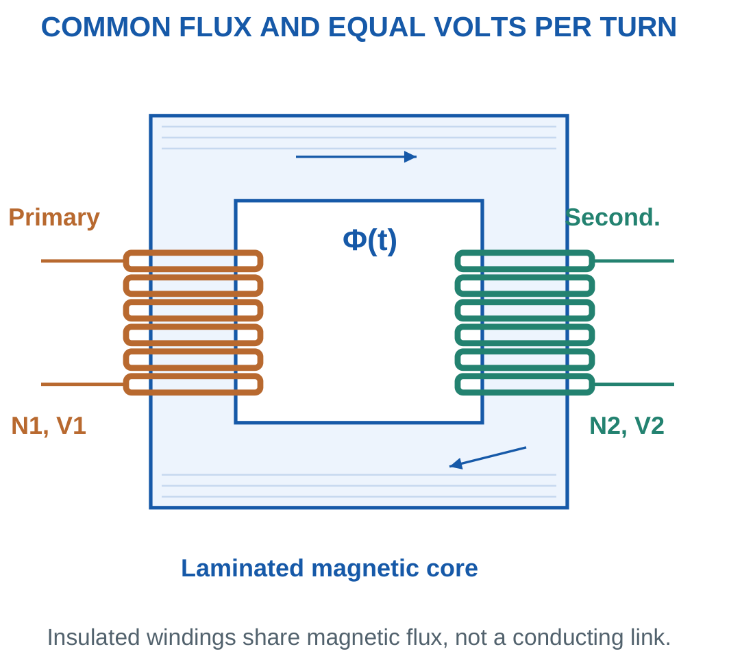
Problem: N1 = 500, N2 = 100, Φm = 2 mWb and f = 50 Hz.
Volts per turn:
Et = 4.44 × 50 × 0.002.
Et = 0.444 V/turn.
Primary EMF:
E1 = 222 V RMS.
Secondary EMF:
E2 = 44.4 V RMS.
Ratio:
E1/E2 = 5 = N1/N2.
If winding drops are neglected, these approximate terminal voltages. Otherwise, the practical circuit determines loaded terminal values.
Toroidal Transformer

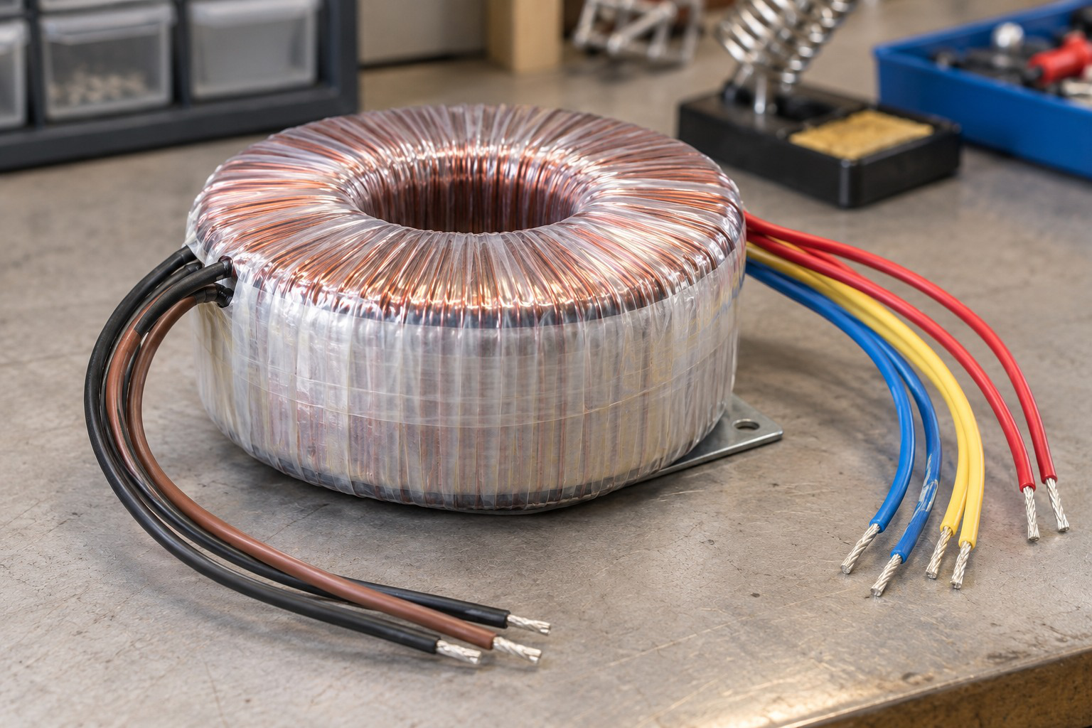
Core geometry and winding arrangement influence construction and magnetic path.
A turns ratio does not imply zero losses in a real device. The practical equivalent separates load-dependent winding effects from excitation effects.
Worked Problem 4.41: A 20:1 EMF Ratio
Problem: N1 = 1000, N2 = 50, Φm = 1 mWb and f = 50 Hz.
Et = 4.44 × 50 × 0.001.
Et = 0.222 V/turn.
E1 = 222 V RMS.
E2 = 11.1 V RMS.
The EMF ratio is 20.
Both windings retain frequency 50 Hz. A voltage-ratio change does not change the number of waveform cycles per second.
Worked Problem 4.42: EMF at 25 Hz
Problem: N1 = 400, N2 = 100, Φm = 3 mWb and f = 25 Hz.
Et = 4.44 × 25 × 0.003.
Et = 0.333 V/turn.
Primary EMF:
133.2 V RMS.
Secondary EMF:
33.3 V RMS.
Ratio:
4.
The same flux links both windings, so the frequency and volts-per-turn terms cancel when forming the ratio.
16. Turns, Core Area and Volts per Hertz
Rearranging the sinusoidal EMF equation gives:
N = E/(4.44fBmA)
Φm = E/(4.44fN)
A = E/(4.44fNBm)
For fixed turns:
Φm ∝ E/f
When winding drops are neglected, applied terminal voltage can approximate E.


A lower operating frequency at unchanged voltage raises flux density. This may increase excitation current and move the core toward saturation.
The calculation identifies the required flux. Acceptability requires the material and device operating limits.
Minimum Whole Turns
If a calculated turn count is the minimum required to stay below a flux-density limit, round upward.
Rounding downward can violate the limit.
After selecting the whole number, recalculate Bm to verify the result.
Do not replace every induced EMF with terminal voltage when the problem includes significant winding impedance drops.
Worked Problem 4.43: Lower Frequency at Fixed EMF
Problem: A winding has 800 turns, E = 230 V RMS, f = 50 Hz and core area 10 cm². Find Bm and the value after a 20% frequency reduction.
A = 0.001 m².
Φm = 230/(4.44 × 50 × 800).
Φm = 0.00129505 Wb.
Bm = Φm/A.
Bm = 1.29505 T.
New frequency is 40 Hz.
Flux-density ratio:
50/40 = 1.25.
Bm,new = 1.61881 T.
The increased density follows from unchanged E, turns and area.
Worked Problem 4.44: Another Frequency Reduction
Problem: E = 120 V, N = 400, f = 60 Hz and A = 8 cm². Frequency falls by 20%.
A = 0.0008 m².
Peak flux:
0.00112613 Wb.
Initial density:
Bm = 1.40766 T.
New frequency:
48 Hz.
The required density rises by 60/48 = 1.25.
Bm,new = 1.75957 T.
A constant-volts-per-hertz change would instead maintain the corresponding flux density under the same approximation.
Ferrite Core and High-Frequency Coil

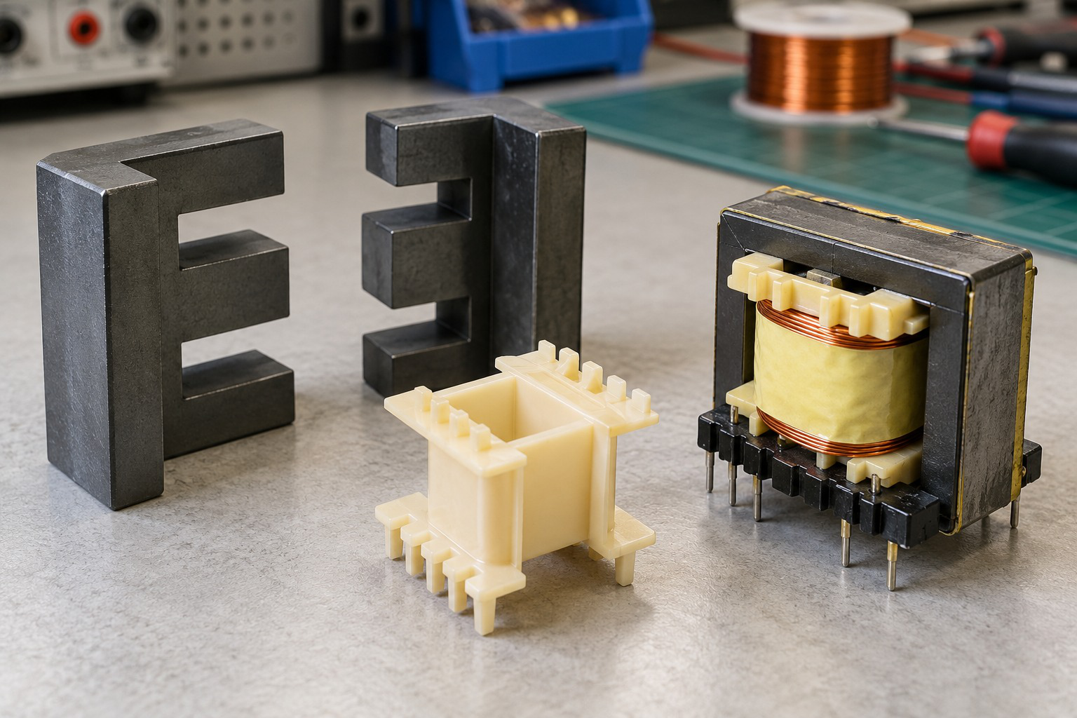
Core material and frequency must suit the selected design.
A ferrite appearance does not establish one universal permissible frequency, flux density or loss. The model and component data determine those values.
Worked Problem 4.45: Minimum Turns at 230 V
Problem: E = 230 V, f = 50 Hz, area is 8 cm² and Bm must not exceed 1.2 T.
Maximum flux:
Φm,max = 1.2 × 0.0008.
Φm,max = 0.00096 Wb.
Continuous minimum turns:
Nmin = 230/(4.44 × 50 × 0.00096).
Nmin = 1079.2.
Round upward:
N = 1080 turns.
Recalculated density:
Bm = 1.19912 T.
This is at or below the specified limit.
Worked Problem 4.46: Minimum Turns at 120 V
Problem: E = 120 V, f = 60 Hz, area is 6 cm² and Bm limit is 1 T.
Maximum flux:
0.0006 Wb.
Continuous minimum turns:
750.751.
Select:
N = 751 turns.
Recalculated peak density:
0.999668 T.
The selected count satisfies the limit. Choosing 750 would not be justified when the calculation specifies a minimum.
Worked Problem 4.47: Minimum Turns at 440 V
Problem: E = 440 V, f = 50 Hz, area is 15 cm² and Bm limit is 1.3 T.
Maximum flux:
1.3 × 0.0015.
0.00195 Wb.
Continuous minimum turns:
1016.4.
Select:
N = 1017 turns.
Actual density:
Bm = 1.29923 T.
The final density check confirms the rounding direction and the area conversion.
17. Ideal Voltage, Current and Turns Ratios
Define the turns ratio:
a = N1/N2
For an ideal transformer:
V1/V2 = a
Therefore:
V2 = V1/a
Ideal apparent power is preserved:
V1I1 = V2I2
Thus:
I1/I2 = 1/a


If a > 1, the selected direction is step-down in voltage.
If a < 1, it is step-up.
Ideal active input and output powers are equal. Load PF is reflected to the input in this ideal model.
Stepping up voltage does not create power because available current changes inversely.
Ratio Definitions
Some texts use k = N2/N1 rather than a.
Both definitions are valid when used consistently. Mixing them reverses voltage or current results.
A signed current relation requires dots and current arrows. The rating examples use RMS magnitudes.
Worked Problem 4.48: Ideal Step-Down with Non-Unity PF
Problem: N1 = 1000, N2 = 100, V1 = 230 V and I2 = 10 A at PF 0.8.
a = 10.
V2 = 230/10.
V2 = 23 V.
I1 = 10/10.
I1 = 1 A.
Apparent power:
S = 230 VA.
Active output:
Pout = 230 × 0.8.
Pout = 184 W.
Ideal active input is also 184 W.
Worked Problem 4.49: Ideal Step-Up
Problem: N1 = 500, N2 = 1000, V1 = 120 V and I2 = 2 A at PF 0.6.
a = 0.5.
V2 = 240 V.
I1 = 4 A.
Output apparent power:
240 × 2.
480 VA.
Input apparent power:
120 × 4.
480 VA.
Active input and output:
288 W.
The higher secondary voltage is accompanied by lower secondary current for equal ideal VA.
Worked Problem 4.50: Unity-PF Load
Problem: N1 = 800, N2 = 200, V1 = 240 V and I2 = 8 A at unity PF.
a = 4.
V2 = 60 V.
I1 = 2 A.
Apparent power:
480 VA.
Active power:
480 W.
The equal numerical watt and VA values follow from unity PF. The turns-ratio relations do not depend on changing PF within this ideal model.
Worked Problem 4.51: A 440 V Primary
Problem: N1 = 1200, N2 = 300, V1 = 440 V and I2 = 5 A at PF 0.9.
a = 4.
Secondary voltage:
110 V.
Primary current:
1.25 A.
Apparent power:
550 VA.
Active power:
495 W.
The ideal input and output active powers agree. A practical model would require adding its specified losses to obtain input active power.
18. VA Rating and Load Current
A single-phase transformer rating is commonly expressed in VA or kVA.
At rated RMS voltages:
I1,rated = Srated/V1,rated
I2,rated = Srated/V2,rated
No √3 factor is used because these are single-phase winding calculations.

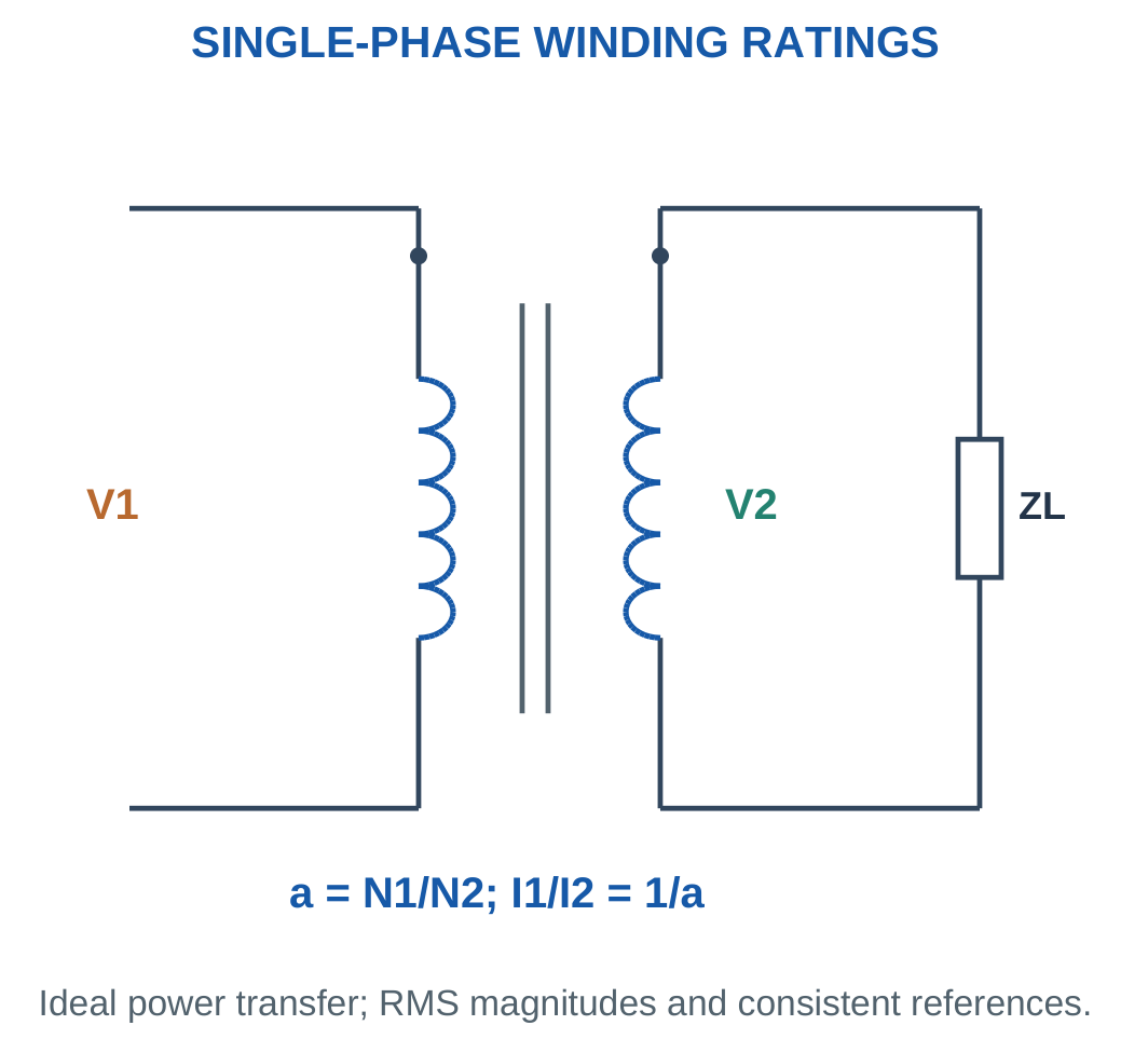
At load fraction x and fixed rated terminal voltage:
Sload = xSrated
I2 = xI2,rated
Useful active output is:
Pout = xSratedPF
A 10 kVA transformer supplies 8 kW at rated kVA and PF 0.8.
The current is determined by VA and voltage, so watt output alone is insufficient to judge winding loading.
Worked Problem 4.52: Rated Currents and Partial Load
Problem: A transformer is rated 10 kVA, 2300/230 V. Find rated currents and operation at 75% load, PF 0.8.
Primary rated current:
10,000/2300.
4.34783 A.
Secondary rated current:
10,000/230.
43.4783 A.
At 75% load:
I2 = 32.6087 A.
Apparent output:
7500 VA.
Active output:
6000 W.
Changing PF at the same apparent load changes useful watts without changing current in this fixed-voltage model.
Worked Problem 4.53: A 5 kVA Rating
Problem: Rating is 5 kVA, 1000/200 V. Operation is at half load and unity PF.
Primary rated current:
5 A.
Secondary rated current:
25 A.
Actual secondary current:
12.5 A.
Apparent output:
2500 VA.
Active output:
2500 W.
Half load here means half rated current or half rated VA at the stated voltage.
Worked Problem 4.54: Full Load at 0.9 PF
Problem: Rating is 20 kVA, 4000/400 V. Find rated currents and full-load output at PF 0.9.
Primary rated current:
20,000/4000.
5 A.
Secondary rated current:
20,000/400.
50 A.
At full load:
Sout = 20,000 VA.
Pout = 18,000 W.
The lower-voltage winding has the larger current rating because both sides correspond to the same apparent-power rating.
Worked Problem 4.55: A 3 kVA Partial Load
Problem: Rating is 3 kVA, 600/120 V. Load fraction is 0.8 at PF 0.6.
Primary rated current:
5 A.
Secondary rated current:
25 A.
Actual secondary current:
20 A.
Apparent output:
2400 VA.
Active output:
1440 W.
The low active watt output does not mean the winding is carrying only 48% of rated current. Its current fraction is 80%.
19. Ideal Transformer Supplying a Complex Load
For secondary load ZL:
V2 = V1/a
I2 = V2/ZL
The load seen from the primary is:
Zin = a²ZL
Then:
I1 = V1/Zin


If ZL = R + jX, both resistance and reactance multiply by a² when referred to the primary.
The impedance angle is unchanged, so an inductive load remains lagging and a capacitive load remains leading.
Complex output power is:
Scomplex,out = V2I2*
For an ideal transformer, the corresponding input active and reactive powers equal the output values.
Physical and Referred Loads
The physical secondary impedance does not change when viewed through an equivalent model.
It still carries its own physical current at its own voltage.
When PF is below one, primary current is not simply Pout/V1. Use apparent power or include PF in the single-phase active-power relationship.
Worked Problem 4.56: Inductive Load Reflected to Primary

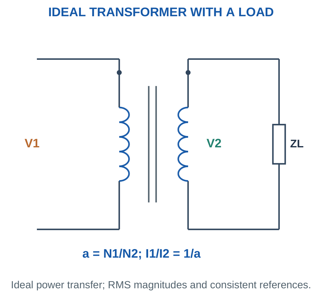
Problem: a = 4, V1 = 240 V at zero degrees and ZL = 6 + j8 Ω.
Secondary voltage:
V2 = 60 V.
Secondary current:
60/(6 + j8).
I2 = 3.6 − j4.8 A.
Primary input impedance:
16(6 + j8).
Zin = 96 + j128 Ω.
Primary current:
I1 = 0.9 − j1.2 A.
Magnitude is 1.5 A.
Complex power:
P + jQ = 216 + j288 VA.
Ideal input and output have the same P and Q.
Worked Problem 4.57: Capacitive Load Reflected to Primary
Problem: a = 5, V1 = 230 V and ZL = 8 − j6 Ω.
Secondary voltage:
46 V.
Secondary current:
I2 = 3.68 + j2.76 A.
Input impedance:
Zin = 200 − j150 Ω.
Primary current:
I1 = 0.736 + j0.552 A.
Magnitude:
0.92 A.
Complex output power:
169.28 − j126.96 VA.
The leading direction is preserved. Negative Q does not represent a negative winding resistance.
Worked Problem 4.58: Step-Up with Complex Load
Problem: a = 0.5, V1 = 120 V and ZL = 30 + j40 Ω.
Secondary voltage:
240 V.
Secondary current:
I2 = 2.88 − j3.84 A.
Input impedance:
0.25(30 + j40).
Zin = 7.5 + j10 Ω.
Primary current:
I1 = 5.76 − j7.68 A.
Magnitude:
9.6 A.
Complex power:
691.2 + j921.6 VA.
The primary current is larger because this selected direction steps voltage upward.
Worked Problem 4.59: A 2:1 Ratio
Problem: a = 2, V1 = 400 V and ZL = 12 + j9 Ω.
Secondary voltage:
200 V.
Secondary current:
I2 = 10.6667 − j8 A.
Input impedance:
Zin = 48 + j36 Ω.
Primary current:
I1 = 5.33333 − j4 A.
Magnitude:
6.66667 A.
Complex power:
2133.33 + j1600 VA.
The input current is the secondary load current referred through the inverse current ratio.
20. Referring Winding Quantities to One Side
With a = N1/N2:
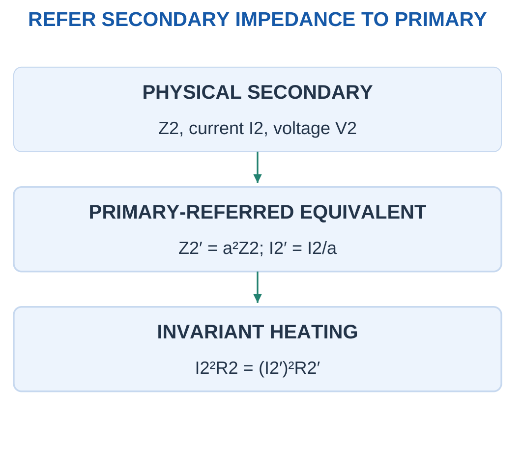
Z2′ = a²Z2
for secondary impedance referred to primary.
For primary impedance referred to secondary:
Z1′ = Z1/a²
Voltage and current scales change consistently:
V2′ = aV2
I2′ = I2/a

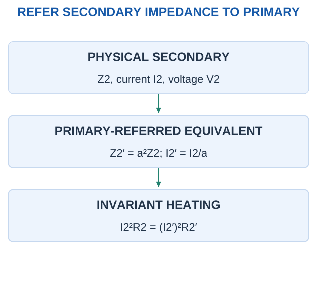
Combined primary-referred series quantities are:
Req,1 = R1 + a²R2
Xeq,1 = X1 + a²X2
Combined secondary-referred quantities are:
Req,2 = R2 + R1/a²
Xeq,2 = X2 + X1/a²
These are electrical winding parameters. They are not magnetic reluctances.
Do Not Add Unmatched Sides
Physical R1 and R2 operate at different current and voltage scales.
Refer them to one side before adding them in one equivalent series circuit.
A useful verification is loss invariance:
I2²R2 = (I2/a)²(a²R2)
The smaller referred current and larger referred resistance produce the same active loss.
Worked Problem 4.60: Equivalent Parameters on Both Sides

Problem: a = 10, R1 = 2 Ω, X1 = 3 Ω, R2 = 0.02 Ω and X2 = 0.04 Ω. Find equivalent parameters and copper loss for I2 = 20 A, neglecting excitation.
Primary-referred:
Req,1 = 4 Ω.
Xeq,1 = 7 Ω.
Secondary-referred:
Req,2 = 0.04 Ω.
Xeq,2 = 0.07 Ω.
Primary current:
I1 = 2 A.
Copper loss:
I1²R1 + I2²R2.
Pcu = 16 W.
Either I1²Req,1 or I2²Req,2 gives the same loss.
Worked Problem 4.61: A 5:1 Equivalent
Problem: a = 5, R1 = 1.5 Ω, X1 = 2 Ω, R2 = 0.08 Ω, X2 = 0.12 Ω and I2 = 10 A.
Primary-referred values:
Req,1 = 3.5 Ω.
Xeq,1 = 5 Ω.
Secondary-referred values:
Req,2 = 0.14 Ω.
Xeq,2 = 0.2 Ω.
With neglected excitation:
I1 = 2 A.
Total copper loss:
14 W.
Reactance is not included as an I²X heat-loss term.
Worked Problem 4.62: A 4:1 Equivalent
Problem: a = 4, R1 = 0.8 Ω, X1 = 1.2 Ω, R2 = 0.05 Ω, X2 = 0.1 Ω and I2 = 15 A.
Primary-referred:
Req,1 = 1.6 Ω.
Xeq,1 = 2.8 Ω.
Secondary-referred:
Req,2 = 0.1 Ω.
Xeq,2 = 0.175 Ω.
Primary load current:
3.75 A.
Copper loss:
22.5 W.
The loss is identical whether calculated using separate physical windings or a consistent referred resistance.
Worked Problem 4.63: A 2:1 Equivalent
Problem: a = 2, R1 = 0.4 Ω, X1 = 0.6 Ω, R2 = 0.1 Ω, X2 = 0.2 Ω and I2 = 8 A.
Primary-referred values:
Req,1 = 0.8 Ω.
Xeq,1 = 1.4 Ω.
Secondary-referred values:
Req,2 = 0.2 Ω.
Xeq,2 = 0.35 Ω.
Primary load current:
4 A.
Total copper loss:
12.8 W.
A referred resistance is an equivalent parameter. The physical winding resistance itself has not changed.
21. Basic Practical Equivalent Circuit
A practical transformer model separates winding effects from excitation effects.
R1 and R2 represent copper resistance.
X1 and X2 represent leakage reactance.
A shunt resistance Rc represents active core loss.
A shunt magnetising reactance Xm represents reactive excitation current.

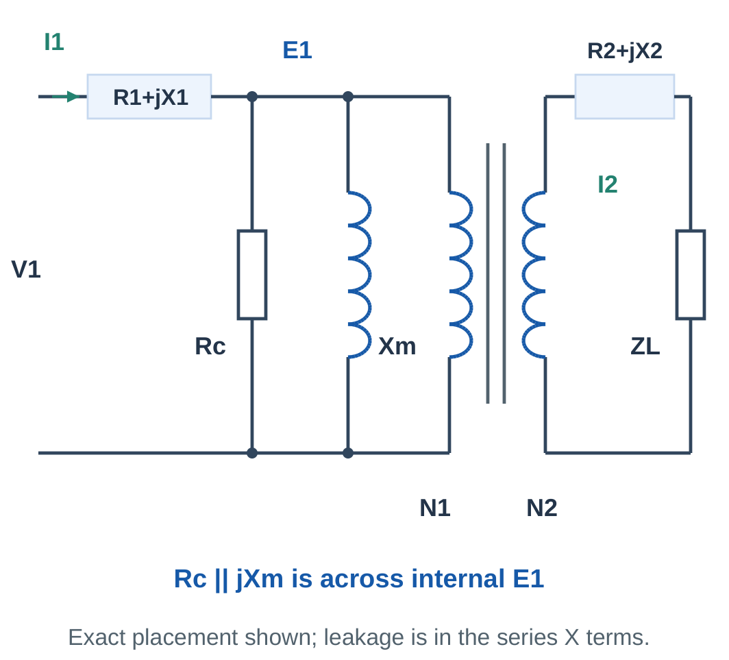
The excitation branch is:
Rc in parallel with jXm
The primary current is the phasor sum:
I1 = I0 + I2′
Primary series impedance carries I1. Secondary series impedance carries I2.
An approximate equivalent circuit can move the excitation branch to the input terminals when primary series drop is small.
State this approximation before using terminal V1 directly across Rc and Xm.
Meaning of the Parameters
Rc is not primary copper resistance.
Xm does not represent a resistor dissipating magnetising watts.
Series leakage reactance and shunt magnetising reactance have different physical roles.
The basic unit calculations use supplied parameters and simple equivalent-circuit relationships. More detailed tests or regulation procedures require their own explicitly supplied model.
Worked Problem 4.64: Supplied Excitation Branch


Problem: Rc = 2300 Ω and Xm = 460 Ω across 230 V RMS.
Core-loss current:
Ic = 230/2300.
Ic = 0.1 A.
Magnetising current:
Im = 230/460.
Im = 0.5 A.
Total current phasor:
I0 = 0.1 − j0.5 A.
Magnitude:
I0 = 0.509902 A.
No-load PF:
0.196116 lagging.
Core-loss power:
Pc = 23 W.
The ideal Xm branch contributes reactive current rather than an additional equal watt loss.
Worked Problem 4.65: A Different Excitation Branch
Problem: Rc = 4000 Ω and Xm = 500 Ω across 200 V.
Ic = 0.05 A.
Im = 0.4 A.
I0 = 0.05 − j0.4 A.
Current magnitude:
0.403113 A.
Power factor:
0.124035 lagging.
Active branch power:
V²/Rc = 200²/4000.
10 W.
The total-current magnitude is found by the square-root sum of component squares, not by adding 0.05 A and 0.4 A.
Worked Problem 4.66: Excitation at 120 V
Problem: Rc = 1200 Ω and Xm = 240 Ω across 120 V.
Core-loss component:
0.1 A.
Magnetising component:
0.5 A.
Total:
I0 = 0.1 − j0.5 A.
Magnitude:
0.509902 A.
PF:
0.196116 lagging.
Core-loss power:
12 W.
The same current components as problem 4.64 do not imply the same watts because the applied voltage is different.
22. No-Load Current and Excitation Parameters
For the approximate input excitation branch:
Ic = V1/Rc
Im = V1/Xm
I0 = Ic − jIm
Magnitude:
|I0| = √(Ic² + Im²)

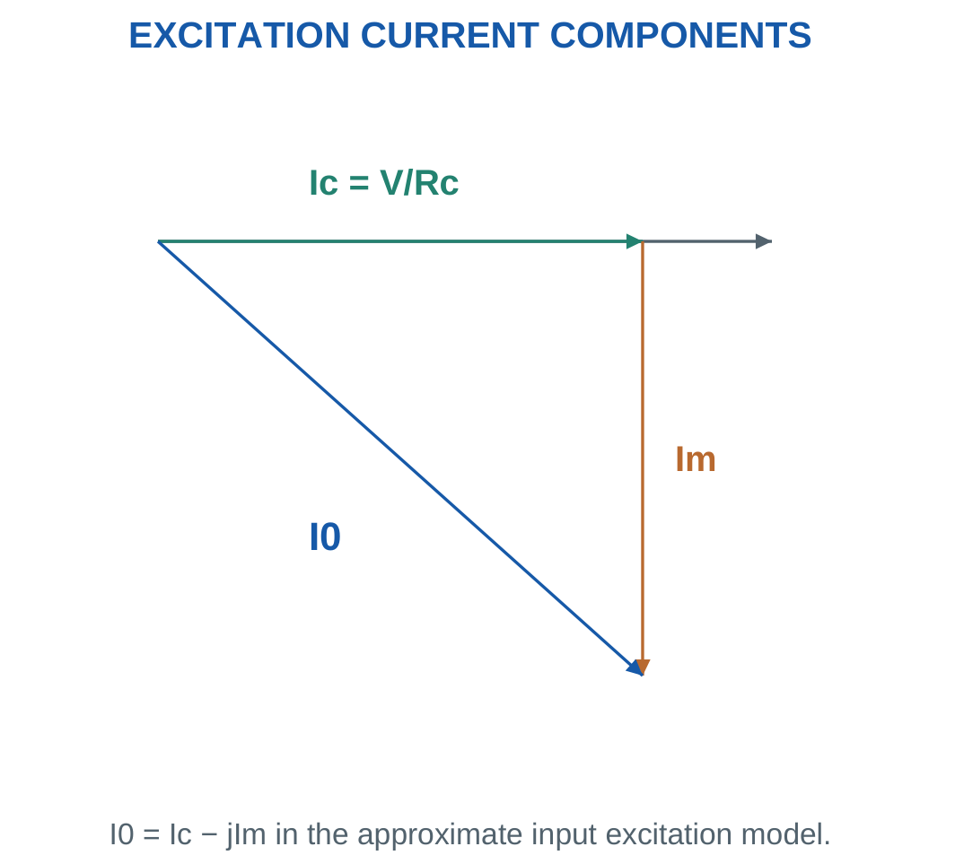
No-load PF is:
PF0 = Ic/I0
If no-load copper loss is neglected:
P0 ≈ Pc = V1²/Rc
From measured V, I0 and P0:
Ic ≈ P0/V
Im = √(I0² − Ic²)
Rc ≈ V/Ic
Xm ≈ V/Im
Ideal and Practical No Load
The exact ideal transformer neglects magnetising current and core loss.
A practical transformer draws excitation with the secondary open.
Finite Rc and Xm do not belong to the zero-excitation ideal model.
If no-load winding loss is explicitly supplied, remove it from the measured active input before identifying the core-loss component.
Worked Problem 4.67: Recover Excitation Parameters
Problem: At open secondary, V = 230 V, I0 = 0.5 A and P0 = 23 W. Neglect no-load winding loss and primary drop.
PF0 = 23/(230 × 0.5).
PF0 = 0.2.
Ic = 23/230.
Ic = 0.1 A.
Im = √(0.5² − 0.1²).
Im = 0.489898 A.
Rc = 230/0.1.
Rc = 2300 Ω.
Xm = 230/0.489898.
Xm = 469.486 Ω.
Worked Problem 4.68: A 200 V No-Load Test Set
Problem: V = 200 V, I0 = 0.4 A and P0 = 40 W under the same approximations.
No-load PF:
0.5.
Core-loss current:
Ic = 0.2 A.
Magnetising current:
Im = 0.34641 A.
Core-loss resistance:
Rc = 1000 Ω.
Magnetising reactance:
Xm = 577.35 Ω.
The measured active power is not assigned to Xm because an ideal reactance has no average active loss.
Worked Problem 4.69: No-Load Parameters at 120 V
Problem: V = 120 V, I0 = 0.3 A and P0 = 12 W.
PF0 = 12/(120 × 0.3).
PF0 = 0.333333.
Ic = 12/120.
Ic = 0.1 A.
Im = √(0.3² − 0.1²).
Im = 0.282843 A.
Rc = 1200 Ω.
Xm = 424.264 Ω.
The square-root result is real because active current does not exceed the measured total-current magnitude.
Worked Problem 4.70: No-Load Parameters at 240 V
Problem: V = 240 V, I0 = 0.6 A and P0 = 48 W.
PF0 = 0.333333.
Ic = 0.2 A.
Im = 0.565685 A.
Rc = 1200 Ω.
Xm = 424.264 Ω.
Relative to the previous example, voltage and current components double while these equivalent impedances remain the same.
23. Equivalent-Circuit Voltage and Copper-Loss Checks
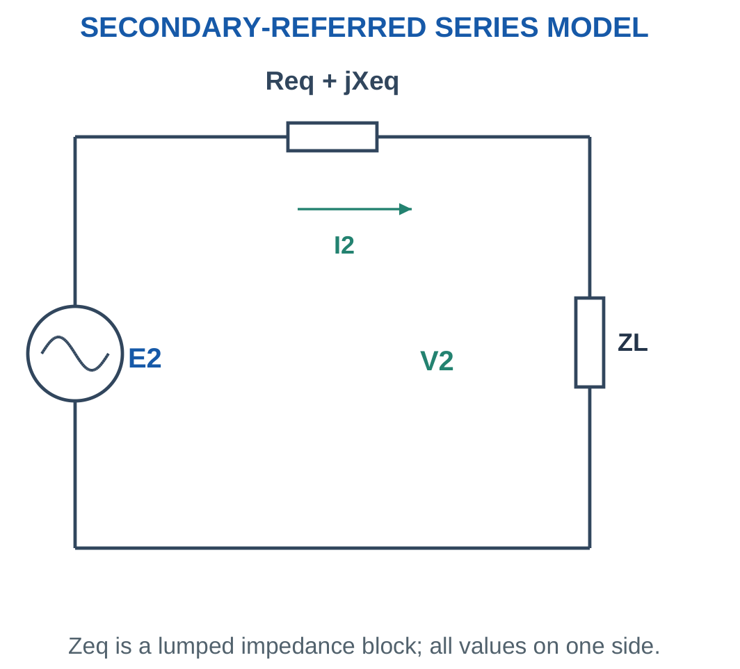
On one reference side, a series impedance gives complex drop:
ΔV = I(Req + jXeq)
Current must be expressed with its phase relative to the load voltage.
For a lagging load, take V2 at zero degrees and I2 at a negative angle.

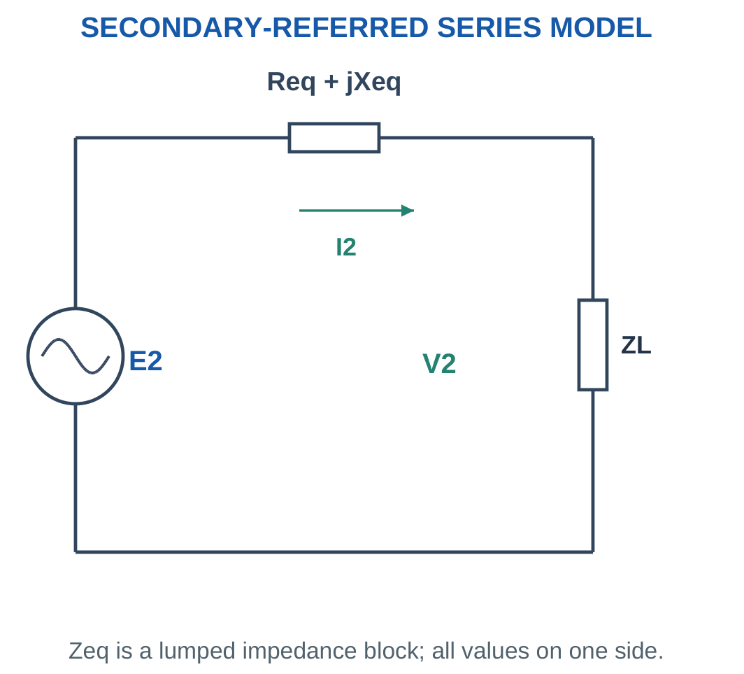
The approximate secondary-referred equation is:
E2 ≈ V2 + I2(Req,2 + jXeq,2)
Add the complex quantities before taking magnitude.
Adding drop magnitude arithmetically is generally wrong because the drop and load voltage need not be in phase.
Copper loss uses the resistance:
Pcu = I2²Req,2
when excitation is neglected.
Use actual winding currents for a more exact separate-winding calculation.
Worked Problem 4.71: Lagging-Load Winding Drop

Problem: V2 = 230 V, I2 = 10 A at 0.8 lagging PF, Req = 0.2 Ω and Xeq = 0.4 Ω.
Current:
I2 = 8 − j6 A.
Drop:
(8 − j6)(0.2 + j0.4).
ΔV = 4 + j2 V.
Internal voltage:
E2 = 234 + j2 V.
Magnitude:
234.009 V.
Angle:
0.489696°.
Copper loss:
10² × 0.2.
20 W.
Worked Problem 4.72: Another Lagging Drop
Problem: V2 = 120 V, I2 = 8 A at 0.6 lagging PF, Req = 0.15 Ω and Xeq = 0.3 Ω.
Current:
I2 = 4.8 − j6.4 A.
Complex drop:
ΔV = 2.64 + j0.48 V.
Internal voltage:
E2 = 122.64 + j0.48 V.
Magnitude:
122.641 V.
Angle:
0.224248°.
Copper loss:
8² × 0.15.
9.6 W.
Leakage reactance contributes to voltage drop but not to average winding heat in the ideal reactance model.
Worked Problem 4.73: Leading-Load Drop
Problem: V2 = 200 V, I2 = 5 A at 0.8 leading PF, Req = 0.3 Ω and Xeq = 0.5 Ω.
Current:
I2 = 4 + j3 A.
Drop:
ΔV = −0.3 + j2.9 V.
Internal voltage:
E2 = 199.7 + j2.9 V.
Magnitude:
199.721 V.
Angle:
0.831978°.
Copper loss:
5² × 0.3.
7.5 W.
The negative real part of the complex drop is compatible with a leading-current phasor and does not imply negative winding resistance.
24. Core Loss and Copper Loss
Core loss consists mainly of hysteresis and eddy-current loss.
Hysteresis loss is associated with repeated magnetisation.
Eddy currents are circulating currents induced within the conducting core material.
Thin insulated laminations reduce the available loop dimensions and help reduce eddy-current loss.

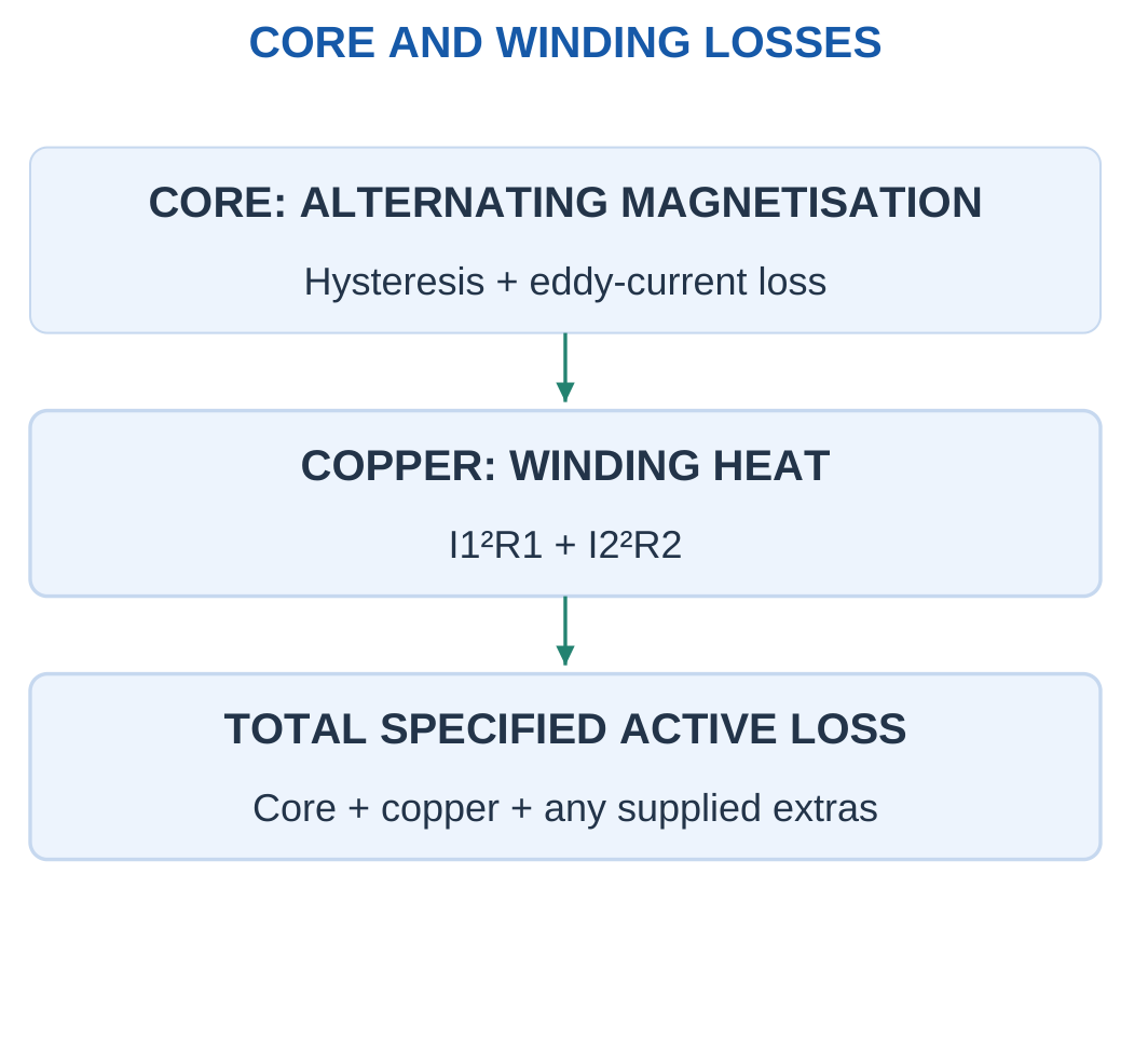
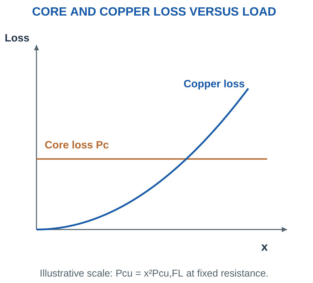
Copper loss is:
Pcu = I1²R1 + I2²R2
At fixed winding resistance it varies approximately as load current squared.
For current fraction x:
Pcu(x) = x²Pcu,FL
Core loss is treated as approximately constant with load when applied voltage and frequency are fixed.
It is not constant under arbitrary changes in voltage, frequency, waveform or material temperature.
Specified Loss Boundary
Real transformers can also have stray, dielectric or auxiliary losses.
Include such terms when supplied. Do not invent additional percentages or omit a stated loss.
The transformer is stationary, so ordinary mechanical friction and windage are not inherent transformer losses. A separately specified cooling auxiliary has its own consumption.
Worked Problem 4.74: Separate Winding Losses
Problem: I1 = 2 A, R1 = 0.8 Ω, I2 = 20 A, R2 = 0.01 Ω and core loss is 30 W.
Primary copper loss:
2² × 0.8.
3.2 W.
Secondary copper loss:
20² × 0.01.
4 W.
Total copper loss:
7.2 W.
Total stated loss:
37.2 W.
The core loss is added as a separate active-power term.
Worked Problem 4.75: Higher Winding Currents
Problem: I1 = 5 A, R1 = 0.4 Ω, I2 = 25 A, R2 = 0.02 Ω and core loss is 60 W.
Primary copper loss:
10 W.
Secondary copper loss:
12.5 W.
Total copper loss:
22.5 W.
Total stated loss:
82.5 W.
Only electrical resistances enter the I²R heating expression. Magnetic reluctance is not substituted into it.
Worked Problem 4.76: Another Loss Balance
Problem: I1 = 1.5 A, R1 = 2 Ω, I2 = 15 A, R2 = 0.03 Ω and core loss is 25 W.
Primary copper loss:
1.5² × 2.
4.5 W.
Secondary copper loss:
15² × 0.03.
6.75 W.
Total copper loss:
11.25 W.
Total stated loss:
36.25 W.
These values correspond to the actual supplied operating currents rather than automatically to full-load conditions.
25. Load Fraction and Copper-Loss Scaling
For a fixed rated-voltage comparison:
x = Actual kVA / Rated kVA
and:
x = Actual current / Rated current
Copper loss therefore follows:
Pcu(x) = x²Pcu,FL
Half rated current produces one quarter full-load copper loss.
A current of 1.25 rated value gives 1.5625 times full-load copper loss under fixed resistance.


If copper loss is known at fraction x1:
Pcu,FL = Pcu(x1)/x1²
At another fraction x2:
Pcu(x2) = Pcu(x1)(x2/x1)²
Use Current or Apparent Load
Copper-loss scaling follows current.
An active-power ratio is not necessarily the current ratio if PF changes.
Determine current fraction from kVA or from P/(SratedPF) at the stated voltage.
A fraction above one can illustrate a mathematical model, but it does not change the equipment’s permitted rating.
Worked Problem 4.77: Recover Full-Load Copper Loss
Problem: Copper loss is 100 W at half rated current. Find full-load loss and total loss at full load if core loss is 60 W.
100 = 0.5²Pcu,FL.
Pcu,FL = 400 W.
At full current:
Pcu = 400 W.
Total loss:
60 + 400.
460 W.
Doubling current from half load to full load multiplies copper loss by four.
Worked Problem 4.78: Change from 75% to 50% Load
Problem: Copper loss is 180 W at 0.75 rated current. Core loss is 80 W.
Full-load copper loss:
180/0.75².
Pcu,FL = 320 W.
At half rated current:
0.5² × 320.
Pcu = 80 W.
Total loss:
160 W.
The direct loss ratio is (0.5/0.75)² = 0.444444.
Core loss does not follow the same load-current-squared scaling in the stated model.
Worked Problem 4.79: Copper Loss at 60% Load
Problem: Full-load copper loss is 240 W and core loss is 100 W.
At x = 0.6:
Pcu = 0.6² × 240.
Pcu = 86.4 W.
Total loss:
100 + 86.4.
186.4 W.
The copper loss is 36% of the full-load value, while active output also depends on the load PF.
26. Efficiency at a Stated Load and Power Factor
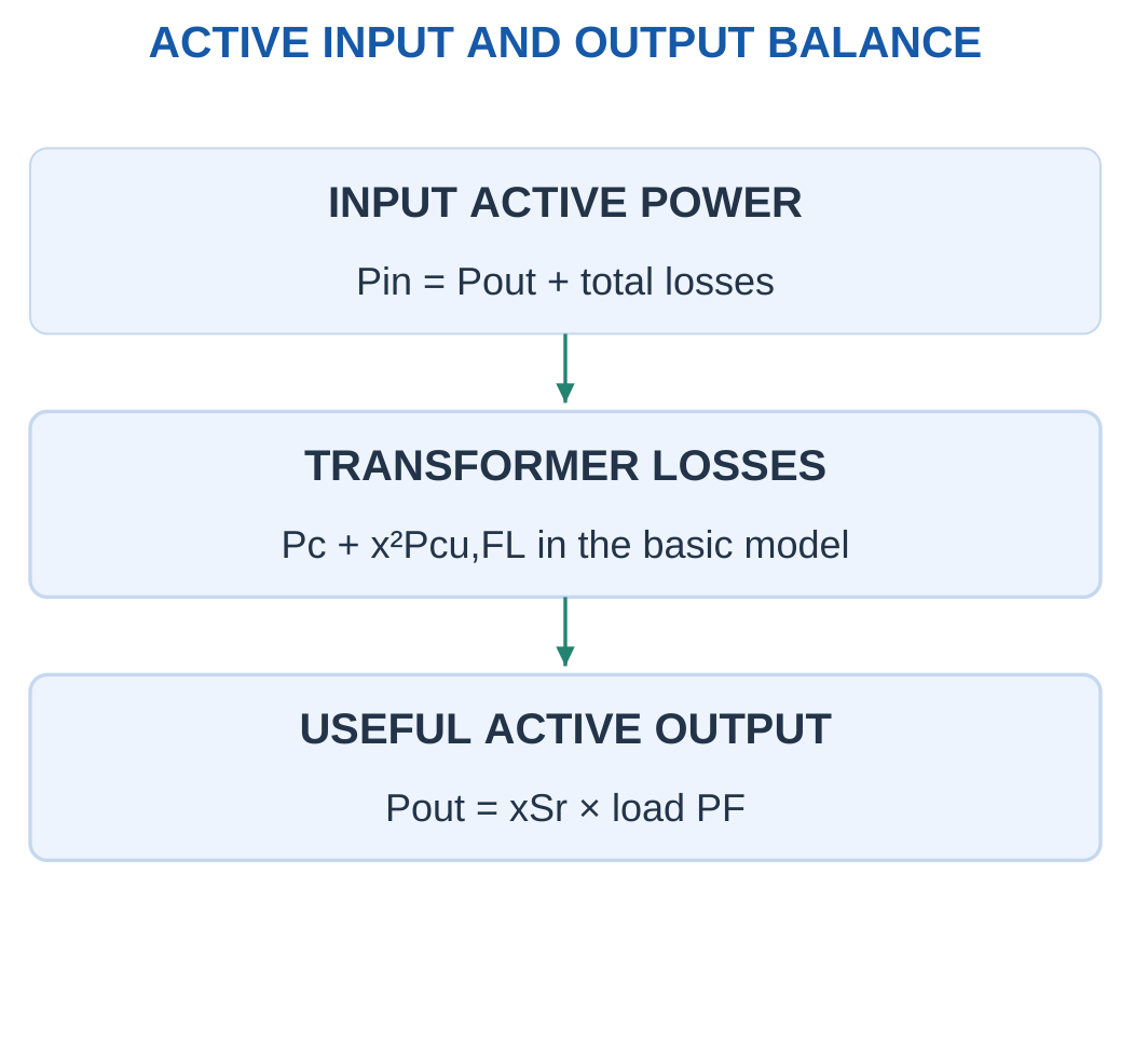
Efficiency is useful active output divided by active input:
η = Pout/Pin
Since:
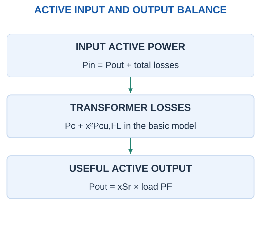
Pin = Pout + Total losses
efficiency becomes:
η = Pout/(Pout + Total losses)
Use active watts in both parts.
For the simplified transformer model:
η = xSratedPF/[xSratedPF + Pc + x²Pcu,FL]

Multiply by 100 to express efficiency as a percentage.
At no useful output and finite core loss, useful-output efficiency is zero.
At the same current fraction, lowering PF reduces active output while the simplified copper and core losses remain unchanged. Efficiency therefore decreases in that comparison.
Input and Output Directions
If Pin and η are known:
Pout = ηPin
If Pout and η are known:
Pin = Pout/η
Loss is the difference.
Use losses corresponding to the same operating point. Do not combine half-load output with unscaled full-load copper loss.
Worked Problem 4.80: Full-Load Efficiency

Problem: Rating is 10 kVA, Pc = 100 W and full-load copper loss is 200 W. Find efficiency at full load and PF 0.8.
Apparent output:
10,000 VA.
Active output:
10,000 × 0.8.
Pout = 8000 W.
Copper loss:
200 W.
Total loss:
300 W.
Input:
Pin = 8300 W.
Efficiency:
8000/8300.
η = 96.3855%.
Transformer Load and Loss Context


Loss and efficiency require a stated operating load and measurement basis.
Useful output watts depend on apparent load and power factor. The winding rating alone does not specify active output for every load.
Worked Problem 4.81: Efficiency at 75% Load
Problem: Rating is 20 kVA, Pc = 180 W and Pcu,FL = 320 W. Load fraction is 0.75 at PF 0.9.
Apparent output:
15,000 VA.
Active output:
13,500 W.
Copper loss:
0.75² × 320.
180 W.
Total loss:
360 W.
Input:
13,860 W.
Efficiency:
97.4026%.
At this operating point copper loss equals core loss, which also identifies the simplified maximum-efficiency condition developed next.
Worked Problem 4.82: Efficiency at Lower Load and PF
Problem: Rating is 3 kVA, Pc = 40 W and Pcu,FL = 80 W. Load fraction is 0.6 and PF is 0.6.
Apparent output:
1800 VA.
Active output:
1080 W.
Copper loss:
0.6² × 80.
28.8 W.
Total loss:
68.8 W.
Input:
1148.8 W.
Efficiency:
94.0111%.
Using 1800 VA as the efficiency numerator would ignore the specified PF and give an incorrect active-power efficiency.
27. Condition for Maximum Efficiency
Assume fixed voltage, frequency, PF and winding resistance.
Let core loss Pc be constant and full-load copper loss be Pcu,FL.
At current fraction x:
Pout = xK
where:
K = SratedPF
Copper loss is:
x²Pcu,FL
Efficiency is:
η = xK/(xK + Pc + x²Pcu,FL)
Maximising this expression gives:
Pc = x²Pcu,FL
Therefore maximum efficiency occurs when variable copper loss equals fixed core loss.

The optimum fraction is:
xmax = √(Pc/Pcu,FL)
At that point, total stated loss is:
2Pc
Optimum Fraction and Efficiency Value
The optimum fraction is independent of PF only when PF is fixed as load varies and the stated loss model applies.
The numerical maximum efficiency still depends on PF through active output.
The calculated optimum may fall below, at or above rated current. A mathematical overload optimum is not an approved operating condition.
Maximum efficiency does not imply zero losses or necessarily full-load operation.
Worked Problem 4.83: Half-Load Optimum


Problem: Rating is 10 kVA, Pc = 100 W, Pcu,FL = 400 W and PF = 0.8.
xmax = √(100/400).
xmax = 0.5.
Copper loss at optimum:
100 W.
Total loss:
200 W.
Active output:
0.5 × 10,000 × 0.8.
4000 W.
Efficiency:
4000/(4000 + 200).
ηmax = 95.2381%.
The optimum lies within the zero-to-rated interval.
Worked Problem 4.84: Optimum at 80% Load
Problem: Rating is 5 kVA, Pc = 80 W, Pcu,FL = 125 W and PF = 1.
xmax = √(80/125).
xmax = 0.8.
Copper loss:
80 W.
Total loss:
160 W.
Active output:
0.8 × 5000.
4000 W.
Efficiency:
96.1538%.
This optimum is also within rated load. It is not necessary for full-load copper loss to equal core loss.
Worked Problem 4.85: A 20 kVA Maximum-Efficiency Calculation
Problem: Rating is 20 kVA, Pc = 200 W, Pcu,FL = 320 W and PF = 0.9.
xmax = √(200/320).
xmax = 0.790569.
Copper loss:
200 W.
Total loss:
400 W.
Active output:
0.790569 × 20,000 × 0.9.
14,230.2 W.
Efficiency:
97.2659%.
The mathematical optimum is within rated current under the specified simplified model.
Worked Problem 4.86: Optimum Above Rated Load
Problem: Rating is 3 kVA, Pc = 90 W, Pcu,FL = 60 W and PF = 0.8.
xmax = √(90/60).
xmax = 1.22474.
At the mathematical optimum:
Pcu = 90 W.
Total loss = 180 W.
Active output:
2939.39 W.
Efficiency:
94.2296%.
The fraction exceeds rated current. Over the permitted zero-to-rated interval, this model is still increasing toward rated load.
The result must not be described as permission to operate continuously above rating.
28. Integrated Transformer Numerical Method
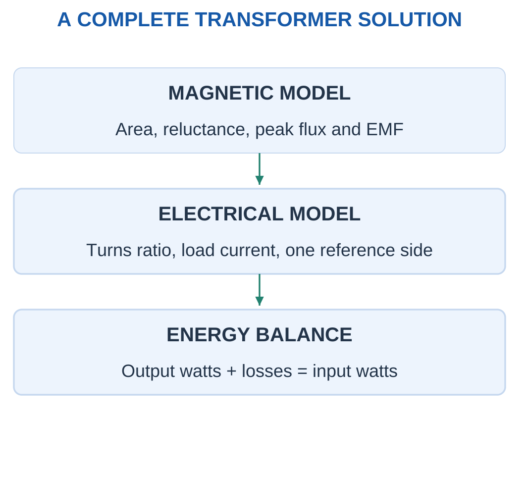
A complete transformer problem may combine magnetic excitation, induced EMF, turns ratio, load current, referred resistance, losses and efficiency.
The first step is selecting the model.
Ideal power equality is not the same as a practical input-output balance containing losses.

Examination Sequence
- Convert area, flux and inductance into SI units.
- Identify peak and RMS quantities.
- Use peak flux in 4.44fNΦm.
- Define a = N1/N2.
- Distinguish active watts from apparent VA.
- Refer impedances before combining them.
- State whether excitation current is neglected.
- Calculate copper loss at actual current fraction.
- Add every specified loss.
- Check input equals useful output plus losses.
Independent Checks
Equal volts per turn checks the common-flux EMF calculation.
The inverse load-current ratio checks ideal power transfer.
Copper-loss invariance checks referral.
Active-power balance checks efficiency.
Magnetic reluctance describes flux excitation. Electrical winding resistance describes copper heating. The quantities are connected through induction but must not be substituted for one another.
Worked Problem 4.87: Integrated Efficiency Calculation


Problem: Rating is 15 kVA, Pc = 150 W, Pcu,FL = 250 W, x = 0.8 and PF = 0.8.
Apparent output:
0.8 × 15,000.
12,000 VA.
Active output:
9600 W.
Copper loss:
0.8² × 250.
160 W.
Total loss:
310 W.
Input:
9910 W.
Efficiency:
96.8718%.
Worked Problem 4.88: Integrated Partial-Load Efficiency
Problem: Rating is 8 kVA, Pc = 90 W, Pcu,FL = 160 W, x = 0.6 and PF = 0.9.
Apparent output:
4800 VA.
Active output:
4320 W.
Copper loss:
0.6² × 160.
57.6 W.
Total loss:
147.6 W.
Input active power:
4467.6 W.
Efficiency:
96.6962%.
The active output rather than apparent output is used in the ratio.
Worked Problem 4.89: Integrated Full-Load Efficiency
Problem: Rating is 12 kVA, Pc = 120 W, Pcu,FL = 180 W, x = 1 and PF = 0.75.
Apparent output:
12,000 VA.
Active output:
9000 W.
Copper loss:
180 W.
Total loss:
300 W.
Input:
9300 W.
Efficiency:
96.7742%.
The input-output difference equals the supplied core loss plus copper loss, confirming the active-power balance.
29. Formula Sheet with Assumptions
| Magnetic Quantity | Relationship |
|---|---|
| Normal uniform flux | Φ = BA |
| Flux density | B = Φ/A |
| Flux linkage | λ = NΦ |
| MMF | F = NI |
| Uniform field strength | H = NI/l |
| Linear material | B = μH |
| Permeability | μ = μ0μr |
| Reluctance | ℜ = l/(μA) |
| Series magnetic circuit | Φ = NI/Σℜ |
| Induced EMF | e = −dλ/dt |
| Fixed-turn induction | e = −N dΦ/dt |
| Linear self-inductance | L = NΦ/I |
| Inductance from reluctance | L = N²/ℜ |
| Self counter-EMF | e = −L di/dt |
| Linear stored energy | Wm = LI²/2 |
| Mutual inductance | M = k√(L1L2) |
| Mutual EMF magnitude | M |
Transformer Formulas
E = 4.44fNΦm
E = 4.44fNBmA
a = N1/N2
V1/V2 = a
I1/I2 = 1/a
S = V1I1 = V2I2
Z2′ = a²Z2
Z1′ = Z1/a²
Req,1 = R1 + a²R2
Req,2 = R2 + R1/a²
Ic = V/Rc
Im = V/Xm
I0 = Ic − jIm
Pc ≈ V²/Rc
The voltage used across Rc and Xm must correspond to their actual placement or the explicitly stated approximate model.
Loss and Efficiency Formulas
Pcu = I1²R1 + I2²R2
Pcu(x) = x²Pcu,FL
Pout = xSratedPF
Pin = Pout + Total losses
η = Pout/Pin
η = xSratedPF/[xSratedPF + Pc + x²Pcu,FL]
xmax = √(Pc/Pcu,FL)
At the simplified optimum:
Pcu = Pc
Unit Reminders
- mWb means 10⁻³ Wb.
- mH means 10⁻³ H.
- cm² means 10⁻⁴ m².
- mm² means 10⁻⁶ m².
- Reluctance is measured in A-turn/Wb.
- Winding resistance is measured in ohms.
- Efficiency compares active watts, not apparent VA.
- Transformer EMF equations use peak flux and RMS EMF.
30. Short Questions with Clear Answers
1. How Do Flux and Flux Density Differ?
Answer: Flux is the total magnetic field crossing a selected surface, measured in webers.
Flux density is flux per normal area, measured in teslas.
Sections in one leakage-free series path can carry the same flux while having different flux densities because their areas differ.
2. Is MMF a Mechanical Force?
Answer: No.
MMF is the magnetic excitation NI, conventionally measured in ampere-turns.
It is not measured in newtons. The historical word force does not make it identical to a mechanical force acting on a body.
3. Why Can a Short Air Gap Dominate Reluctance?
Answer: Air permeability is much lower than the stated permeability of a typical magnetic core.
Gap reluctance is g/(μ0A). Its small length can therefore be offset by the much smaller permeability.
The core MMF should still be retained unless neglecting it is explicitly allowed.
4. Does Reluctance Directly Dissipate Φ²ℜ Watts?
Answer: No.
The electrical-magnetic analogy is not a power-loss identity.
Actual core losses involve hysteresis and eddy-current mechanisms. Electrical winding resistance produces I²R heating.
Reluctance describes the excitation needed to establish flux.
5. Can Steady Flux Induce EMF in a Stationary Coil?
Answer: Not when flux linkage is constant.
Faraday’s law depends on the rate of change of linkage.
A nonzero constant linkage has zero derivative and therefore zero induced EMF under the stationary fixed-turn model.
6. What Does Lenz’s Law Oppose?
Answer: The induced effect opposes the change of linkage that produces it.
It does not simply state that induced flux always opposes the original flux.
When linkage decreases, the induced effect can act to maintain it. The relevant opposition is to the change.
7. Why Does Inductance Scale with Turns Squared?
Answer: For fixed linear reluctance, flux is NI/ℜ.
Flux linkage introduces another factor N.
Therefore L = N²/ℜ.
Doubling turns makes inductance four times as large when the path and permeability remain represented by the same reluctance.
8. What Is the Largest Allowed Coupling Coefficient?
Answer: For passive reciprocal linear coils with M expressed as a positive magnitude, k cannot exceed one.
The mutual-inductance magnitude must not exceed √(L1L2).
A larger calculated value indicates incompatible data, a unit error or a model outside the stated assumptions.
9. Does an Ideal Transformer Change Frequency?
Answer: No.
Ordinary ideal transformation preserves source frequency.
The turns ratio changes voltage and current levels. Additional power-electronic stages in a larger product are separate devices and are not part of the basic transformer ratio model.
10. Why Does a Practical Transformer Draw No-Load Current?
Answer: It requires magnetising current to establish the alternating flux and active current to supply core loss.
The exact ideal transformer neglects both effects.
Finite excitation parameters therefore belong to a practical or approximate model rather than a zero-excitation ideal model.
11. Why Is Peak Flux Used in the EMF Equation?
Answer: The sine-wave derivative and RMS conversion produce E = 4.44fNΦm.
The quantity Φm is the flux amplitude.
Substituting RMS flux without conversion gives the wrong value. The coefficient already includes the conversion from the resulting peak EMF to RMS EMF.
12. Why Are Winding Impedances Referred Before Addition?
Answer: The windings operate at different voltage and current scales.
Referring through the square of the turns ratio puts their effects on one consistent side.
The procedure preserves the equivalent voltage-current and power relationships. Adding physical values from unmatched sides does not form a valid single-side circuit.
13. Does Half Load Mean Half Copper Loss?
Answer: No.
At half rated current, copper loss is one quarter of full-load loss because it varies with current squared in the fixed-resistance model.
If PF changes, an active-watt ratio is not automatically the same as the current fraction.
14. Why Is Transformer Rating Given in kVA Rather Than Only kW?
Answer: Winding current and applied voltage strongly govern heating and magnetic operation.
Load PF determines useful active watts for a given VA.
Two loads at the same kVA can therefore produce different active outputs while imposing the same RMS current at the same voltage.
15. When Is Efficiency Maximum in the Simple Model?
Answer: At fixed PF and supply conditions, maximum efficiency occurs when variable copper loss equals fixed core loss.
The fraction is √(Pc/Pcu,FL).
The mathematical optimum must still be compared with the permitted operating range. Maximum efficiency does not necessarily occur at full load.
31. Complete Examination Answers
1. Derive the Simple Magnetic-Circuit Equation
Answer:
For a uniform linear magnetic path, Ampère’s law gives:
NI = Hl
The material relation is:
B = μH
Flux through a uniform normal section is:
Φ = BA
Therefore:
H = B/μ = Φ/(μA).
Substitute into the excitation equation:
NI = Φl/(μA).
Define reluctance:
ℜ = l/(μA)
Hence:
NI = Φℜ
and:
Φ = NI/ℜ
For several sections in series with negligible leakage, the same main flux passes through each section. Individual MMF requirements add:
NI = Φ(ℜ1 + ℜ2 + …)
If areas differ, calculate each B separately even though flux is common.
The derivation assumes the stated permeability model and main-path approximation. A nonlinear material can instead require B–H data at each section’s operating point.
The unit of reluctance is A-turn/Wb. It does not represent an electrical resistor dissipating a magnetic analogue of I²R.
2. Explain Faraday’s Law and Lenz’s Law
Answer:
Faraday’s law states that changing flux linkage produces induced EMF:
e = −dλ/dt
For N turns linking the same changing flux:
e = −N dΦ/dt
Over a uniform finite interval:
eavg = −NΔΦ/Δt
The full signed change must be used. A reversal from positive to negative flux includes both parts of the change.
Lenz’s law explains the negative sign. The induced effect opposes the linkage change producing it.
This does not require every numerical terminal voltage to be negative because terminal and winding references determine the displayed sign.
Mechanical motion is not necessary. A stationary coil experiences induction when its linked field changes with time.
Constant linkage gives zero induced EMF.
For sinusoidal flux:
Φ = Φm sinωt
the induced counter-EMF is:
e = −NωΦm cosωt
EMF magnitude is greatest at flux zero crossings and zero at flux extremes.
The physical law should therefore be interpreted through rate of change rather than the size of the instantaneous flux alone.
3. Explain Self-Inductance and Mutual Inductance
Answer:
Self-inductance relates a coil’s own current to its flux linkage.
For a linear model:
L = λ/I = NΦ/I
Using the magnetic-circuit equation:
L = N²/ℜ
A larger reluctance gives a smaller inductance. A larger number of turns increases inductance with the square of turns when reluctance is unchanged.
The induced counter-EMF is:
e = −L di/dt
The passive terminal voltage is +L di/dt. These signs use different references.
Mutual inductance describes linkage in a second winding produced by current in the first.
Its induced-EMF magnitude is:
|e2| = M|di1/dt|
For reciprocal linear coils:
M = k√(L1L2)
with 0 ≤ k ≤ 1 under the positive-magnitude convention.
Winding dots and current references determine mutual polarity.
Stored magnetic energy in a linear ideal inductor is:
Wm = LI²/2
This energy can be returned. It is not automatically a dissipative core or copper loss.
Nonlinear magnetic models require more careful treatment of linkage-current slope and stored-energy integrals.
4. Explain Transformer Construction and Operation
Answer:
A two-winding transformer has insulated primary and secondary windings linked by common alternating magnetic flux.
The magnetic core provides a low-reluctance path. Laminations restrict eddy-current loops.
Insulation separates turns, windings and core.
AC voltage applied to the primary establishes alternating flux. Faraday’s law produces induced EMFs in both windings.
When winding drops are small, the primary induced counter-EMF approximately balances the applied voltage.
At open secondary, a practical transformer draws excitation current. One component establishes the field, while another supplies active core loss.
The exact ideal model neglects these components.
When the load draws secondary current, the primary draws an additional load-current component. Its ampere-turns oppose the secondary load ampere-turns so that the main operating flux remains primarily set by applied voltage per frequency and turns.
The secondary voltage supplies load current and power. The device does not create energy.
Ordinary transformer action preserves frequency. Voltage and current levels change according to turns ratio, while a practical device has losses and terminal-voltage drops.
The induced EMFs E1 and E2 must be distinguished from terminal voltages V1 and V2 whenever the practical model includes winding impedance.
5. Derive the Transformer EMF Equation and Ideal Ratios
Answer:
Assume common sinusoidal flux:
Φ = Φm sinωt
Faraday’s law gives peak induced-EMF magnitude:
Em = NωΦm
Since ω = 2πf:
Em = 2πfNΦm
For a sinusoid, RMS magnitude is peak divided by √2:
E = Em/√2
Therefore:
E = √2πfNΦm
Using the conventional rounded coefficient:
E = 4.44fNΦm
For two windings linking common flux:
E1 = 4.44fN1Φm
E2 = 4.44fN2Φm
Dividing:
E1/E2 = N1/N2
Define:
a = N1/N2
In the ideal low-drop model:
V1/V2 = a
Ideal apparent-power transfer gives:
V1I1 = V2I2
Therefore the RMS current magnitudes satisfy:
I1/I2 = 1/a
Voltage step-up is accompanied by current step-down for the same transferred VA.
The common-flux, sinusoidal and ideal-loss assumptions are part of the derivation. A practical loaded transformer requires its equivalent-circuit drops and losses.
6. Explain the Basic Practical Equivalent Circuit
Answer:
The practical equivalent circuit separates series winding effects from shunt excitation effects.
R1 and R2 model winding copper resistance.
X1 and X2 model leakage reactance.
The shunt resistance Rc models active core loss.
The shunt reactance Xm models magnetising current.
In the exact circuit, the excitation branch is across internal E1 after the primary series impedance.
Primary current is the phasor sum of excitation current and referred secondary load current.
An ideal transformer in the equivalent circuit links the two reference sides. The physical secondary series impedance carries secondary current.
An approximate circuit may move the excitation branch to the input when primary drop is small. That approximation allows terminal V1 to be used across Rc and Xm.
Secondary impedance referred to primary is multiplied by a². Primary impedance referred to secondary is divided by a².
All impedances must be on one reference side before they are added.
Copper-loss invariance provides a check: the referred current and referred resistance must reproduce the same active loss as the physical winding.
Rc is not winding copper resistance. Xm is not an active-loss resistance. Series leakage reactance and shunt magnetising reactance must not be confused.
7. Explain Transformer Losses and Load Efficiency
Answer:
Core loss consists mainly of hysteresis and eddy-current loss.
At fixed voltage and frequency, the basic efficiency model treats it as approximately constant with load.
Copper loss is:
Pcu = I1²R1 + I2²R2
At fixed resistance and current fraction x:
Pcu = x²Pcu,FL
Useful active output is:
Pout = xSratedPF
Input active power equals output plus all specified losses.
For the two-loss model:
Pin = xSratedPF + Pc + x²Pcu,FL
Therefore:
η = xSratedPF/[xSratedPF + Pc + x²Pcu,FL]
Use active watts rather than apparent VA in the efficiency ratio.
At the same current fraction, lowering PF reduces useful output watts while the simplified losses remain unchanged. Efficiency therefore falls in that comparison.
At no useful output, finite no-load losses produce zero useful-output efficiency.
Losses from different operating points must not be combined without scaling. In particular, copper loss must be evaluated at the actual current fraction.
Additional supplied stray, dielectric or auxiliary losses are included in the balance. They should neither be invented nor silently omitted.
8. Derive the Maximum-Efficiency Condition
Answer:
At fixed supply conditions and fixed PF, let:
K = SratedPF
Then output is xK and copper loss is x²Pcu,FL.
Efficiency is:
η = xK/(xK + Pc + x²Pcu,FL)
For x greater than zero, divide numerator and denominator by x:
η = K/[K + Pc/x + xPcu,FL]
Maximising efficiency is equivalent to minimising:
Pc/x + xPcu,FL
Differentiate with respect to x:
d/dx = −Pc/x² + Pcu,FL
At the stationary optimum:
−Pc/x² + Pcu,FL = 0.
Therefore:
x²Pcu,FL = Pc
Thus variable copper loss equals fixed core loss.
The optimum fraction is:
xmax = √(Pc/Pcu,FL)
Total loss at that point is 2Pc.
The fraction is independent of a fixed PF under the stated model, but maximum-efficiency value depends on PF because useful active output includes it.
The calculated optimum must be checked against the allowed operating range. An optimum above rated current is a mathematical result, not a revised equipment rating.
Final Revision Checklist
Magnetic Quantities
- Flux is measured in Wb.
- Flux density is measured in T.
- Linkage includes the turn count.
- MMF is NI in ampere-turns.
- H uses mean magnetic path length.
- Reluctance is l/(μA).
- Series sections share flux, not necessarily B.
- An air-gap MMF is added separately.
- B–H data replace an unsupported constant-permeability assumption.
Induction and Inductance
- Induced EMF depends on linkage change.
- Use final minus initial flux.
- A reversal uses the complete signed change.
- Constant linkage gives zero induced EMF.
- Sinusoidal EMF is in quadrature with flux.
- Self-inductance is NΦ/I in the linear model.
- Inductance scales with N² at fixed reluctance.
- Mutual polarity requires winding references.
- Stored energy is not automatically heat loss.
Transformer Calculations
- Define a = N1/N2.
- Use peak flux in the EMF equation.
- Use RMS winding voltage and current in rating calculations.
- Frequency is unchanged in ordinary ideal transformation.
- Voltage and current ratios are inverse.
- Single-phase VA calculations do not use √3.
- Active watts include load PF.
- Referring impedance requires a².
- Add winding parameters only on one reference side.
- State excitation approximations.
Loss and Efficiency Checks
- Copper loss uses resistance, not impedance magnitude.
- Core loss and copper loss are separate.
- Copper loss scales with current squared.
- Load fraction follows current or kVA at fixed voltage.
- Efficiency uses active output and active input.
- Check Pin = Pout + losses.
- Maximum efficiency has Pcu = Pc in the stated model.
- Check whether the optimum fraction is within rated operation.
Final Calculation Habit
Identify the model before choosing a formula.
Convert units, define references and distinguish peak from RMS quantities.
Keep magnetic reluctance, electrical resistance and reactance separate.
Verify volts per turn, inverse current ratio, referred-loss invariance and active-power balance wherever applicable.
Report the requested quantity with its unit, operating condition and any necessary sign interpretation.