
University: Dr. A.P.J. Abdul Kalam Technical University (AKTU)
Programme: B.Tech First Year, Semester I & II
Course Codes: AEE101A / AEE201A
Branches: Common to All
Unit: V — Electrical Machines and Emerging Electrical Systems
Introduction
Electrical Machines and Emerging Electrical Systems connects motor principles and useful mechanical output with electronically commutated drives, induction-motor operation, solar photovoltaic characteristics and responsible laboratory practice.
An electrical machine must be understood through its electrical circuit, magnetic field, mechanical motion and energy balance. A voltage equation can establish armature current, but it does not automatically establish shaft output. A torque equation can describe electromagnetic force, but useful mechanical power also requires speed.
The same discipline applies to photovoltaic systems. Irradiance is incident optical power per area, electrical output is a simultaneous voltage-current product, and energy requires a time basis. Keeping these definitions separate prevents many common numerical errors.
Syllabus Coverage
- DC motor operating principle.
- Force on a current-carrying conductor.
- Brushed DC motor construction.
- Back EMF and the armature equation.
- Developed torque and mechanical power.
- DC motor power balance and efficiency.
- Starting-current control.
- Armature-voltage, resistance and field-control concepts.
- DC motor types and applications.
- BLDC motor construction and electronic commutation.
- Electrical frequency and mechanical speed.
- Three-phase induction motor construction.
- Rotating magnetic field.
- Synchronous speed, pole count and slip.
- Rotor frequency, induced EMF and reactance.
- Induction-motor torque and power conversion.
- Solar photovoltaic systems.
- Single-diode PV equivalent model.
- Current–voltage and power–voltage characteristics.
- Maximum-power point and fill factor.
- Irradiance and cell-temperature effects.
- Matched series-parallel arrays.
- PV efficiency and energy calculations.
- Electrical laboratory safety and stored energy.
Topic Map
| Topic | PDF Pages |
|---|---|
| Motor power and DC construction | 2–5 |
| DC back EMF, torque and power balance | 5–11 |
| Starting, speed control and motor types | 11–15 |
| BLDC concepts and commutation | 15–19 |
| Induction motor, rotating field and speed | 19–25 |
| Induction torque and applications | 25–30 |
| PV system and single-diode model | 30–33 |
| I–V, P–V, MPP and condition effects | 33–38 |
| Matched arrays and PV energy | 38–41 |
| Laboratory safety and complete revision | 41–47 |
How to Study This Unit
- Identify electrical input, developed mechanical power and shaft output.
- Convert rpm into rad/s before using P = Tω.
- Separate shunt line current from armature current.
- State the flux assumption in torque and speed ratios.
- Distinguish mechanical revolutions from electrical cycles.
- Insert slip as a fraction rather than a percentage.
- Keep air-gap power separate from stator electrical input.
- Use simultaneous PV voltage and current values.
- Define whether the PV model represents a cell, module or array.
- Follow the approved supervised laboratory procedure.
Symbols and Conventions
DC motor equations use steady positive motoring references unless stated otherwise. AC supply quantities are RMS values. N denotes mechanical rpm, ω denotes rad/s and s denotes slip fraction.
PV parameters describe the stated cell or module level. Irradiance and cell temperature remain explicit. Simplified models and losses must be identified before numerical substitution.
A symbol can have different meanings in different sections. P means pole count in the DC generated-EMF equation, while power is usually identified by a descriptive subscript. A means armature parallel paths in that equation, but illuminated area in PV efficiency calculations.
Similarly, Ns means synchronous speed in induction-motor calculations, while a series-count symbol in a PV equation may count cells or modules. The meaning must be defined at the point of use.
Main Principle
A useful solution connects its equation to the correct energy boundary. Torque, watts, volt-amperes and energy describe different quantities. Units and a physical check help establish whether they have been combined correctly.
The examples use supplied idealised parameters and stated losses. They do not assume the performance of an unspecified commercial motor, converter or PV installation.
1. Electrical Machines and Energy Conversion
An electric motor converts electrical input into mechanical output. A generator converts mechanical input into electrical output.
Electromagnetic interaction transfers energy between a current-carrying electrical system and a moving mechanical system. A practical machine also has losses, so useful output is smaller than input.


Mechanical Power
Mechanical power is:
Pmech = Tω
where:
- Pmech is mechanical power in watts.
- T is torque in N·m.
- ω is angular speed in rad/s.
If speed N is supplied in rpm:
ω = 2πN/60
Therefore:
T = 60Pmech/(2πN)
If power is in kilowatts, the familiar approximation is:
T ≈ 9550P(kW)/N(rpm)
This shortcut already includes the unit conversion. It must be used with kilowatts and rpm in the stated places.
Model Boundaries
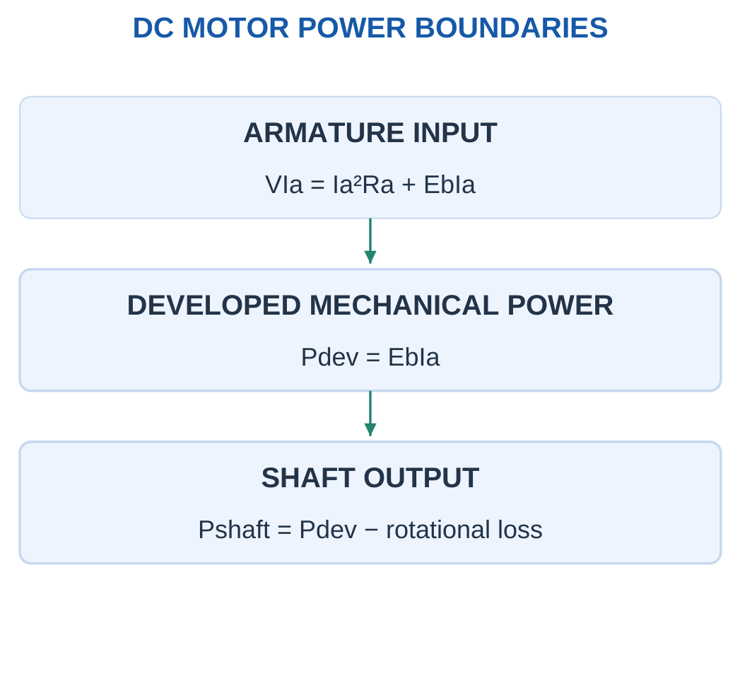
A motor can have electromagnetic developed power and a smaller shaft output. Friction, windage and other rotational losses lie between these quantities.
Pshaft = Pdev − Prot
Always identify which power and torque the question requests. Developed torque uses developed power, while shaft torque uses useful shaft output.
A motor’s electrical input is a further upstream quantity. It includes the power eventually lost electrically and mechanically.
Electrical and Mechanical Speed
Mechanical speed counts shaft revolutions. Electrical frequency counts magnetic or electrical cycles.
Their relationship depends on pole-pair count and machine type. A speed in rpm cannot be substituted directly as rad/s or electrical hertz.
For example, 1500 rpm is 25 revolutions per second. Its angular speed is 157.08 rad/s. Electrical frequency additionally depends on the relevant pole-pair relationship.
Worked Problem 5.1: Shaft Torque from Speed and Output Power
Problem: A motor delivers 1500 W shaft output at 1500 rpm. Find angular speed and shaft torque, and recover power from the answer.
Step 1: Convert mechanical speed.
ω = 2πN/60 = 2π × 1500/60 = 157.08 rad/s
Step 2: Use Pshaft = Tshaftω.
Tshaft = 1500/157.08 = 9.5493 N·m
Step 3: Check with the approximate kW/rpm shortcut.
Tshaft ≈ 9550 × 1.5/1500 = 9.55 N·m
Step 4: Recover power.
Pshaft = Tshaftω ≈ 1500 W
The stated watts are useful shaft output. Electrical input would require efficiency or loss information. Dividing watts directly by rpm would omit the required 2π/60 conversion.
Worked Problem 5.2: Shaft Torque at 1440 rpm
Problem: A motor delivers 4000 W shaft output at 1440 rpm. Find angular speed and shaft torque.
Step 1: Convert speed.
ω = 2π × 1440/60 = 150.796 rad/s
Step 2: Calculate shaft torque.
Tshaft = 4000/150.796 = 26.5258 N·m
Step 3: Use the approximate formula as a check.
Tshaft ≈ 9550 × 4/1440 = 26.5278 N·m
Step 4: Recover output power.
Pshaft = 26.5258 × 150.796 ≈ 4000 W
The small difference between exact and shortcut results comes from rounding the conversion constant. Both calculations use shaft power and therefore give shaft torque.
Motor and Electronic Drive in an EV

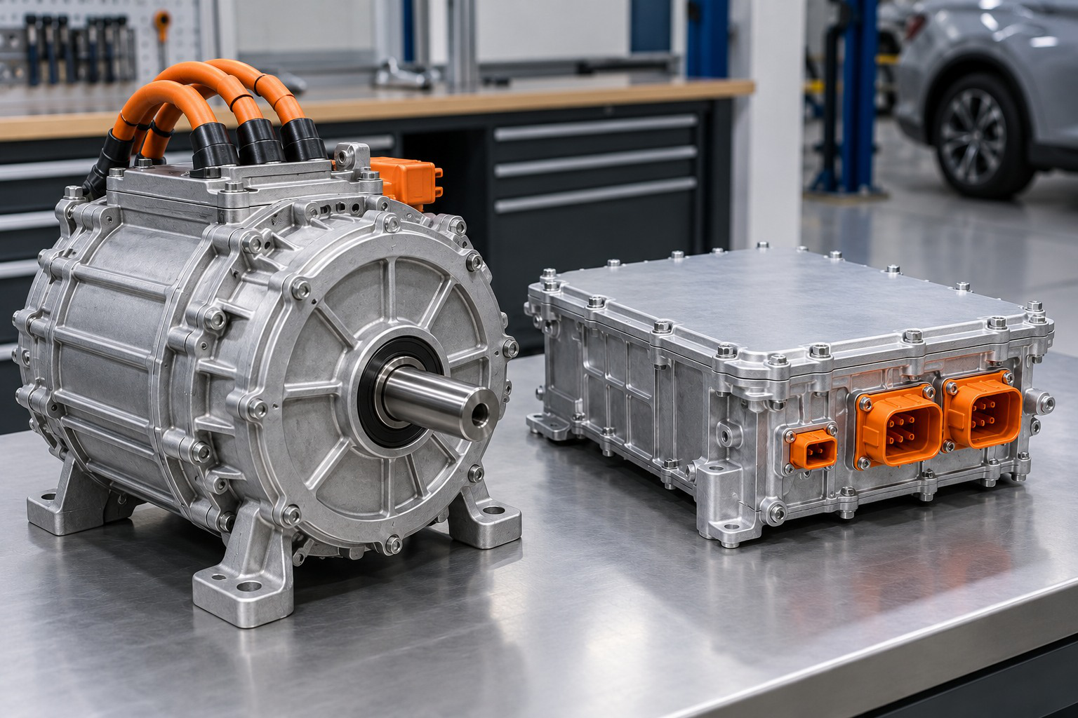
An electric drive connects electrical input with controlled motor operation and shaft output. Useful mechanical power, developed power and losses are different quantities.
The selected motor and drive model defines the torque-speed and energy calculation. A photograph identifies hardware but does not establish a numerical efficiency, torque constant or complete operating envelope.
2. DC Motor Principle and Force Direction
A current-carrying conductor in a magnetic field experiences force.
For a straight active conductor:
F = BIl sin θ
where θ is the angle between conductor-current direction and magnetic-field direction.
Maximum magnitude occurs when the directions are perpendicular:
F = BIl

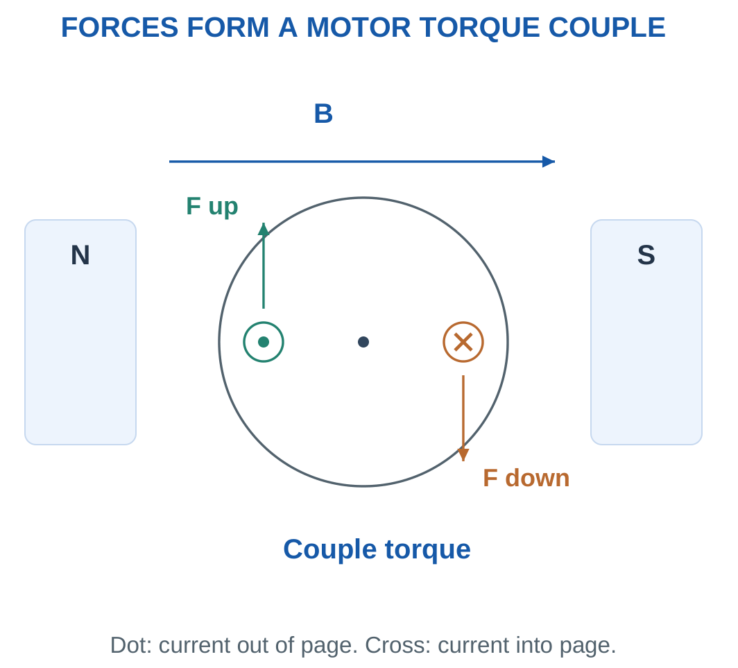
Formation of Torque
In a motor, conductor forces act at a distance from the shaft and produce torque.
For one tangential force F acting at radius r:
T = Fr
For two equal opposite forces whose moments aid:
Ttotal = 2Fr
The forces may cancel as a translational resultant while their moments add about the shaft.
Fleming’s left-hand rule can indicate relative field, current and force directions. The rule supports a defined geometry; the field and conductor-current references must still be identified.
Commutation
A DC armature needs its current pattern switched as the rotor turns so that useful torque continues in the intended direction.
A brushed machine uses a commutator and brushes for this switching. The commutator is not itself the source of the main magnetic field.
Reversing armature current alone or field direction alone reverses torque direction in the ideal model. Reversing both leaves the torque direction unchanged.
Force and Torque Are Different
Force is measured in newtons. Torque is force multiplied by its perpendicular lever arm and is measured in N·m.
The radius is therefore essential. A force value alone does not determine shaft torque.
If the conductor is not perpendicular to the magnetic field, the sin θ factor must be included before calculating the corresponding moment.
Worked Problem 5.3: Force Couple on Two Active Conductors
Problem: Two opposite armature sides each have active length 0.2 m, current 8 A and perpendicular field 0.5 T. Each tangential force acts at radius 0.06 m. Find force per side and total couple torque.
Step 1: With θ = 90°:
F = BIl = 0.5 × 8 × 0.2 = 0.8 N
Step 2: One side contributes:
Fr = 0.8 × 0.06 = 0.048 N·m
The opposite side contributes the same torque magnitude.
Step 3: Add the two moments.
Ttotal = 2Fr = 0.096 N·m
Step 4: Interpret direction.
Reversing field or current reverses the torque reference. Reversing both leaves the torque sense unchanged. This sign change does not introduce an additional force-magnitude factor.
Worked Problem 5.4: Force Couple with Different Dimensions
Problem: Each active side has length 0.15 m, current 5 A and perpendicular field 0.8 T. Each force acts at radius 0.04 m.
Step 1:
F = 0.8 × 5 × 0.15 = 0.6 N
Step 2:
Fr = 0.6 × 0.04 = 0.024 N·m
Step 3:
Ttotal = 2 × 0.024 = 0.048 N·m
Step 4: Distinguish the result types.
Force per side is 0.6 N, while total couple torque is 0.048 N·m. The two opposite forces have no net translational force, but they produce a rotational effect.
Worked Problem 5.5: Force Couple at Higher Current
Problem: Two opposite sides each have length 0.25 m, current 12 A and perpendicular field 0.4 T. Radius is 0.05 m.
Step 1:
F = 0.4 × 12 × 0.25 = 1.2 N
Step 2:
Fr = 1.2 × 0.05 = 0.06 N·m
Step 3:
Ttotal = 2 × 0.06 = 0.12 N·m
Step 4: Check the geometry.
The factor two represents the two active sides. It should not be added again if a supplied complete-machine torque constant already includes all conductor contributions.
Additional Concept Checks
A force of 2 N acting tangentially at 0.05 m gives 0.1 N·m torque. Reporting 2 N·m would omit the lever arm.
A conductor at 30° to the magnetic field has half the perpendicular-force magnitude because sin 30° = 0.5. The angular factor changes force; the appropriate lever arm then determines torque.
3. Brushed DC Motor Construction
The stator provides the main field using field windings or permanent magnets.
The armature is the rotating part carrying conductors in a laminated core. The shaft carries mechanical output. Brushes make sliding electrical contact with commutator segments connected to the armature winding.

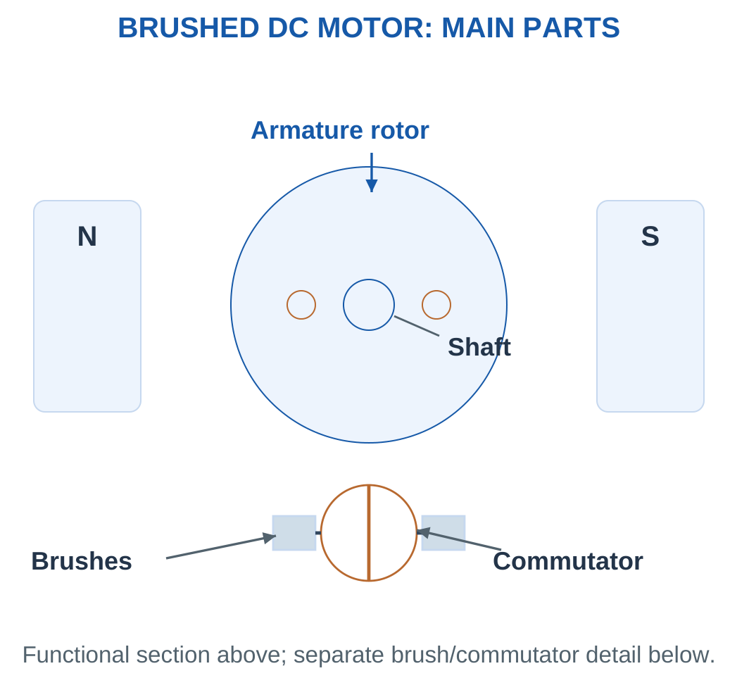
Main Parts and Functions
- Stator: Establishes the stationary magnetic structure and main field.
- Armature core: Supports the active conductors and provides a magnetic path.
- Armature winding: Carries current involved directly in energy conversion.
- Commutator: Changes the connection of rotating armature conductors.
- Brushes: Connect stationary terminals to the rotating commutator.
- Shaft: Transfers useful mechanical output.
- Bearings: Support rotation and maintain alignment.
- Insulation: Separates conductors and structural metal where required.
The commutator changes which rotating conductors are connected to the external DC terminals. This permits an approximately unidirectional developed torque.
In the rotor conductors themselves, current directions change as the winding moves through the magnetic structure.
Laminations and Losses
Laminations reduce large circulating eddy-current paths in parts exposed to changing flux.
Bearings support rotation but introduce mechanical loss. Windage and other rotational effects also reduce useful shaft output below electromagnetic developed power.
These losses belong to the relevant power balance rather than to the armature resistance term alone.
Field and Armature Connections
The field circuit establishes flux. The armature circuit carries current directly involved in energy conversion.
In a shunt motor, the field and armature are parallel branches. In a series motor, the same current flows through field and armature.
The functional cross-section is not a complete manufacturer’s assembly drawing. Its labels identify the parts needed to understand the equations and the difference between brushed and brushless commutation.
4. Back EMF and the Armature Equation
As a DC motor rotates, its armature conductors cut magnetic flux and generate an EMF opposing the applied supply.
This induced voltage is back EMF, Eb.
With steady current, negligible brush drop and armature resistance Ra:
V = Eb + IaRa
Therefore:
Eb = V − IaRa
Ia = (V − Eb)/Ra

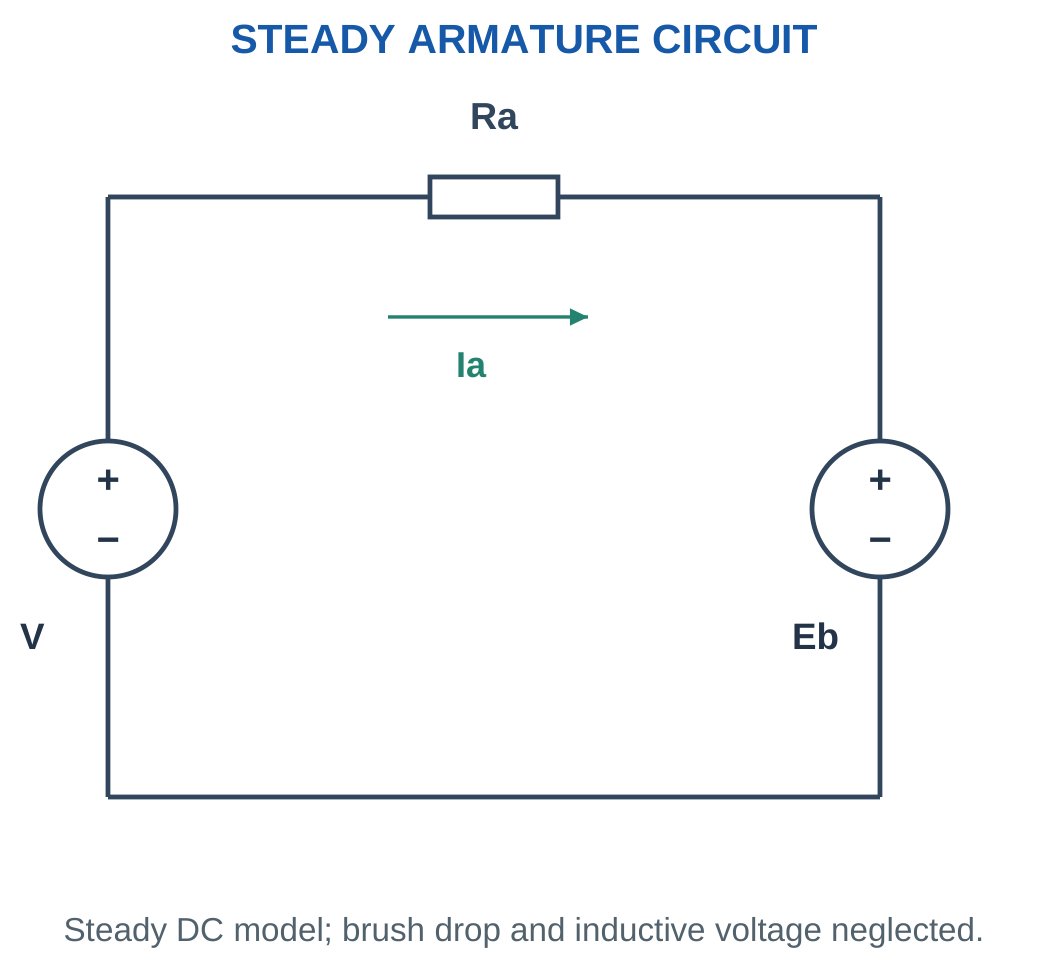
Starting Condition
At the instant of starting, speed and rotational back EMF are approximately zero.
The resistance-only estimate becomes:
Istart = V/Ra
Direct application of full voltage can therefore produce a large current in the low armature resistance. Current limiting or an appropriate starter/controller is required.
The steady equation identifies the need for control. A detailed instantaneous starting waveform would additionally require armature inductance and controller behaviour.
Response to Increased Load
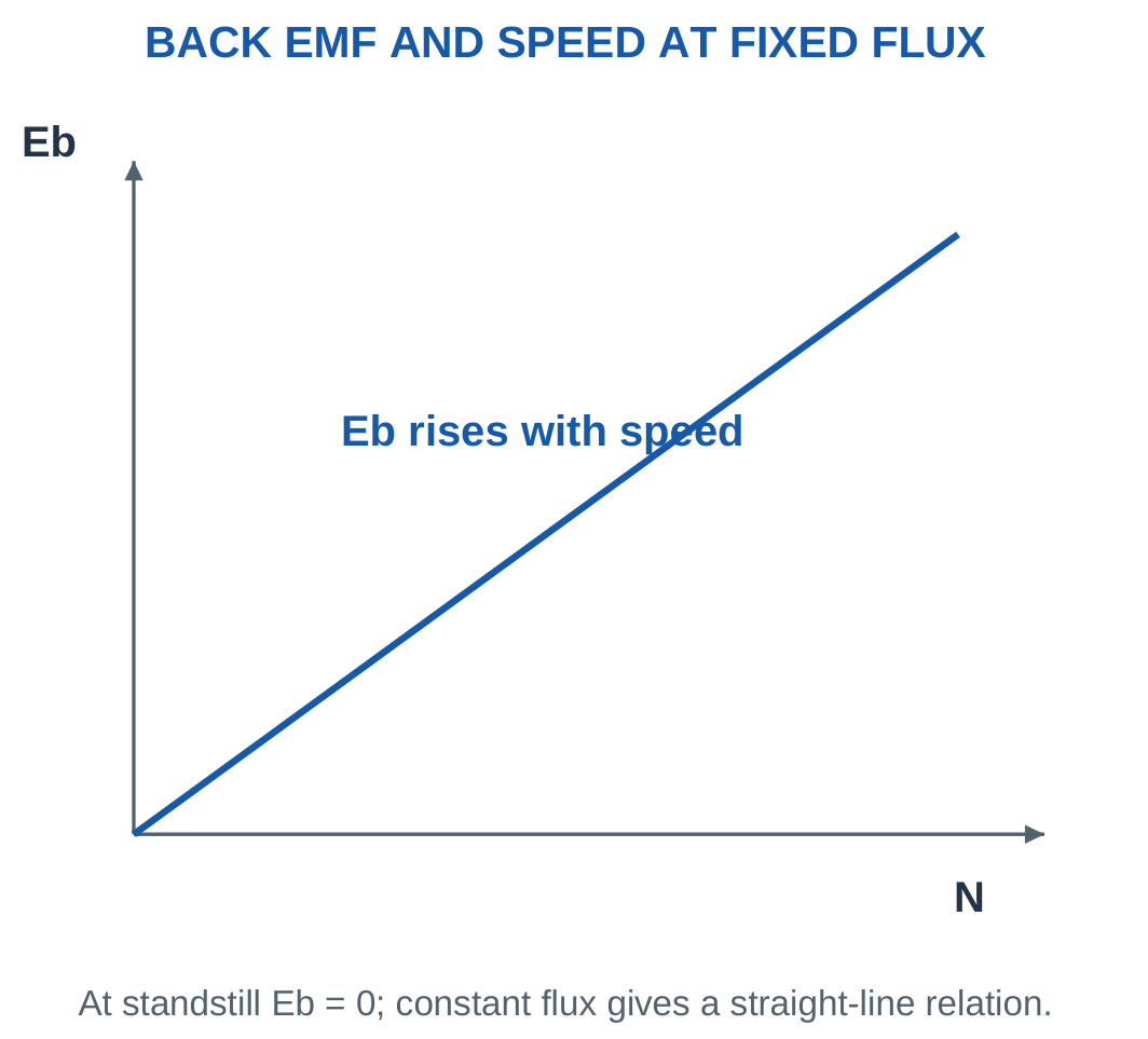
When mechanical load increases, speed initially tends to fall. This reduces Eb at approximately constant flux.
The larger difference V − Eb raises armature current and developed torque, allowing a new operating point within the machine’s limits.
This describes natural electrical feedback. It does not mean every overload can be supported indefinitely.
Back EMF and Power
Multiplying the voltage equation by current gives:
VIa = EbIa + Ia²Ra
Here:
- VIa is armature input.
- EbIa is developed conversion power.
- Ia²Ra is armature copper heat.
Back EMF is therefore not a loss by itself. If brush voltage drop or inductance is supplied, its corresponding voltage term must also be included.
Worked Problem 5.6: Back EMF and Armature Power Split

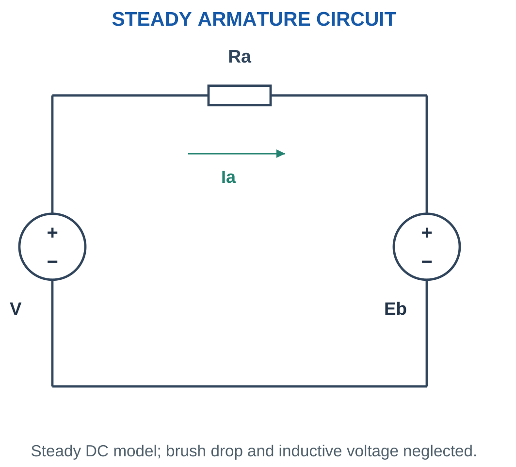
Problem: A steady DC armature takes 20 A from 220 V. Ra = 0.5 Ω and speed is 1000 rpm. Find back EMF, copper loss, developed power and developed torque.
Step 1: Armature resistance drop is:
IaRa = 20 × 0.5 = 10 V
Eb = 220 − 10 = 210 V
Step 2: Calculate input and copper heat.
VIa = 220 × 20 = 4400 W
Ia²Ra = 20² × 0.5 = 200 W
Step 3: Calculate developed conversion power.
Pdev = EbIa = 210 × 20 = 4200 W
Check: 200 + 4200 = 4400 W.
Step 4: Convert speed and calculate torque.
ω = 104.72 rad/s
Tdev = 4200/104.72 = 40.107 N·m
Shaft torque would require specified rotational losses.
Worked Problem 5.7: Armature Power at 240 V
Problem: A motor armature takes 25 A from 240 V. Ra = 0.4 Ω and speed is 1200 rpm.
Step 1:
IaRa = 25 × 0.4 = 10 V
Eb = 240 − 10 = 230 V
Step 2:
VIa = 240 × 25 = 6000 W
Ia²Ra = 25² × 0.4 = 250 W
Step 3:
Pdev = 230 × 25 = 5750 W
The sum of copper loss and developed power is 6000 W.
Step 4:
ω = 125.664 rad/s
Tdev = 5750/125.664 = 45.757 N·m
This is developed torque because the power is taken before rotational losses.
Worked Problem 5.8: Armature Power at 120 V
Problem: An armature takes 10 A from 120 V. Ra = 0.8 Ω and speed is 1500 rpm.
Step 1:
IaRa = 10 × 0.8 = 8 V
Eb = 120 − 8 = 112 V
Step 2:
VIa = 120 × 10 = 1200 W
Ia²Ra = 10² × 0.8 = 80 W
Step 3:
Pdev = 112 × 10 = 1120 W
Check: 80 + 1120 = 1200 W.
Step 4:
ω = 157.08 rad/s
Tdev = 1120/157.08 = 7.13014 N·m
A complete motor efficiency would additionally need the complete input boundary and downstream losses.
Worked Problem 5.9: Armature Power at 900 rpm
Problem: An armature takes 15 A from 200 V. Ra = 0.6 Ω and speed is 900 rpm.
Step 1:
IaRa = 15 × 0.6 = 9 V
Eb = 200 − 9 = 191 V
Step 2:
VIa = 200 × 15 = 3000 W
Ia²Ra = 15² × 0.6 = 135 W
Step 3:
Pdev = 191 × 15 = 2865 W
Check: 135 + 2865 = 3000 W.
Step 4:
ω = 94.2478 rad/s
Tdev = 2865/94.2478 = 30.3986 N·m
Back EMF is below supply voltage, consistent with the stated positive-current motoring reference.
5. Back EMF, Flux and Speed
For a DC armature:
Eb = PΦZN/(60A)
where:
- P is pole count.
- Φ is flux per pole in Wb.
- Z is the total number of active armature conductors.
- N is speed in rpm.
- A is the number of parallel armature paths.
The same relation can be expressed as:
Eb = KeΦω
when machine geometry is collected into Ke and angular speed is in rad/s.

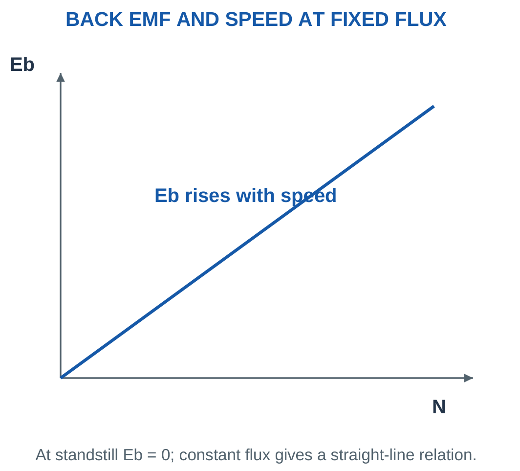
Comparing Two Conditions
For fixed geometry:
N ∝ Eb/Φ
Therefore:
N2/N1 = (Eb2/Eb1)(Φ1/Φ2)
First obtain each back EMF from its own armature voltage balance.
A larger flux at the same speed gives larger back EMF. With a fixed applied voltage, current and speed must adjust according to the load and controller.
Constants and Units
A volts-per-rpm constant differs numerically from a volts-per-rad/s constant. Use the speed unit associated with the supplied constant.
P in the construction equation means pole count. A means parallel paths, rather than conductor area. Identifying these symbols avoids incorrect substitutions from another topic.
Worked Problem 5.10: EMF from Construction Data
Problem: A DC armature has four poles, flux 0.02 Wb per pole, 600 active conductors and four parallel paths. Find back EMF at 1000 rpm and at 20% higher speed with unchanged flux.
Step 1:
Eb = 4 × 0.02 × 600 × 1000/(60 × 4)
Eb = 200 V
Step 2: With fixed flux and geometry, EMF is proportional to speed.
N2 = 1.2 × 1000 = 1200 rpm
Step 3:
Eb2 = 1.2 × 200 = 240 V
Step 4: Interpret the generated value.
This is a back-EMF calculation, not automatic equality with terminal voltage under load. If voltage and resistance were supplied, current would follow from V − Eb = IaRa.
Motor Cutaway: Field and Armature

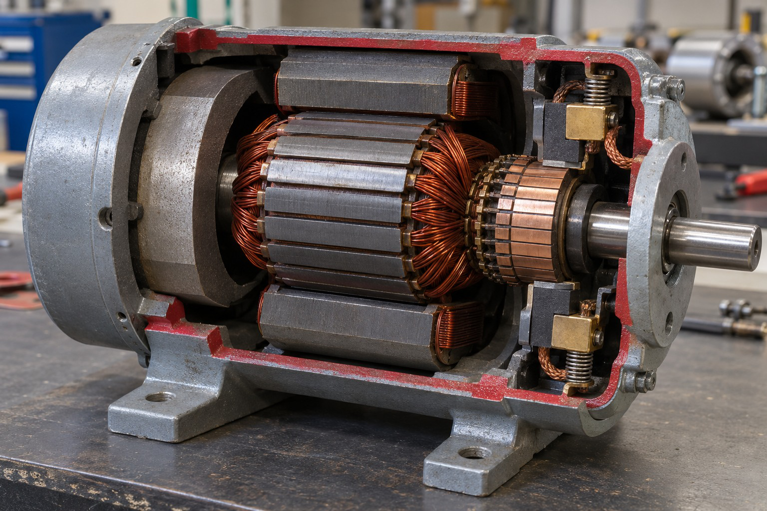
A DC motor connects electrical input, back EMF, developed mechanical power and losses. Developed torque and shaft torque can differ.
The conceptual diagram establishes reference directions. Physical construction helps locate the field and armature, but a numerical model is still required to calculate performance.
Worked Problem 5.11: Six-Pole Armature EMF
Problem: An armature has six poles, flux 0.025 Wb per pole, 720 conductors and six parallel paths. Find EMF at 800 rpm and after a 20% speed increase.
Step 1:
Eb = 6 × 0.025 × 720 × 800/(60 × 6)
Eb = 240 V
Step 2:
N2 = 1.2 × 800 = 960 rpm
Step 3:
Eb2 = 1.2 × 240 = 288 V
Step 4: Retain the operating reference.
A computed back EMF above the supply would not fit the same positive-current motoring assumption. The generated-EMF equation alone does not determine every loaded terminal condition.
6. Developed Torque and Converted Power
Electromagnetic developed power in the simple DC motor model is:
Pdev = EbIa
It is electrical power converted internally into mechanical form before rotational losses.
For nonzero speed:
Tdev = Pdev/ω
Combining the EMF equation with ω = 2πN/60 gives:
Tdev = [PZ/(2πA)]ΦIa
Thus:
Tdev = KΦIa
for a fixed machine.

Flux Assumptions
If flux is constant:
Tdev ∝ Ia
For an unsaturated series field where Φ is proportional to Ia:
Tdev ∝ Ia²
Saturation changes the flux-current relation and therefore changes the square-law approximation.
Developed and Shaft Torque
If rotational loss is supplied:
Pshaft = EbIa − Prot
Tshaft = Pshaft/ω
Tdev = EbIa/ω
Reporting the same torque for both ignores the supplied mechanical loss.
At zero speed, Pdev/ω becomes indeterminate if both numerator and denominator are zero. The direct torque relation explains finite starting torque.
Worked Problem 5.12: Developed Torque and Shaft Torque
Problem: Back EMF is 200 V, armature current 15 A, speed 1000 rpm and rotational loss 200 W. Find developed and shaft powers and torques.
Step 1:
Pdev = 200 × 15 = 3000 W
Step 2:
Pshaft = 3000 − 200 = 2800 W
Step 3:
ω = 104.72 rad/s
Tdev = 3000/104.72 = 28.6479 N·m
Step 4:
Tshaft = 2800/104.72 = 26.738 N·m
The torque difference, 1.90986 N·m, corresponds to the 200 W rotational loss at this speed.
Worked Problem 5.13: Torque at 1500 rpm
Problem: Eb = 120 V, Ia = 10 A, N = 1500 rpm and rotational loss is 100 W.
Step 1:
Pdev = 120 × 10 = 1200 W
Step 2:
Pshaft = 1200 − 100 = 1100 W
Step 3:
ω = 157.08 rad/s
Tdev = 1200/157.08 = 7.63944 N·m
Step 4:
Tshaft = 1100/157.08 = 7.00282 N·m
The torque difference is 0.63662 N·m. Both torques use the same speed, while their power boundaries differ.
Worked Problem 5.14: Torque at 1200 rpm
Problem: Eb = 230 V, Ia = 20 A, N = 1200 rpm and rotational loss is 300 W.
Step 1:
Pdev = 230 × 20 = 4600 W
Step 2:
Pshaft = 4600 − 300 = 4300 W
Step 3:
ω = 125.664 rad/s
Tdev = 4600/125.664 = 36.6056 N·m
Step 4:
Tshaft = 4300/125.664 = 34.2183 N·m
The torque difference, 2.38732 N·m, represents the supplied rotational-loss power at this speed.
Worked Problem 5.15: Torque at 800 rpm
Problem: Eb = 80 V, Ia = 8 A, N = 800 rpm and rotational loss is 60 W.
Step 1:
Pdev = 80 × 8 = 640 W
Step 2:
Pshaft = 640 − 60 = 580 W
Step 3:
ω = 83.7758 rad/s
Tdev = 640/83.7758 = 7.63944 N·m
Step 4:
Tshaft = 580/83.7758 = 6.92324 N·m
The torque difference is 0.716197 N·m. Neglecting the 60 W loss would incorrectly make shaft output equal to developed power.
7. DC Motor Power Balance and Efficiency
For the armature-only steady model:
Parmature = VIa
Pcu,armature = Ia²Ra
Pdev = EbIa
The balance:
VIa = Ia²Ra + EbIa
follows from multiplying the voltage equation by current.
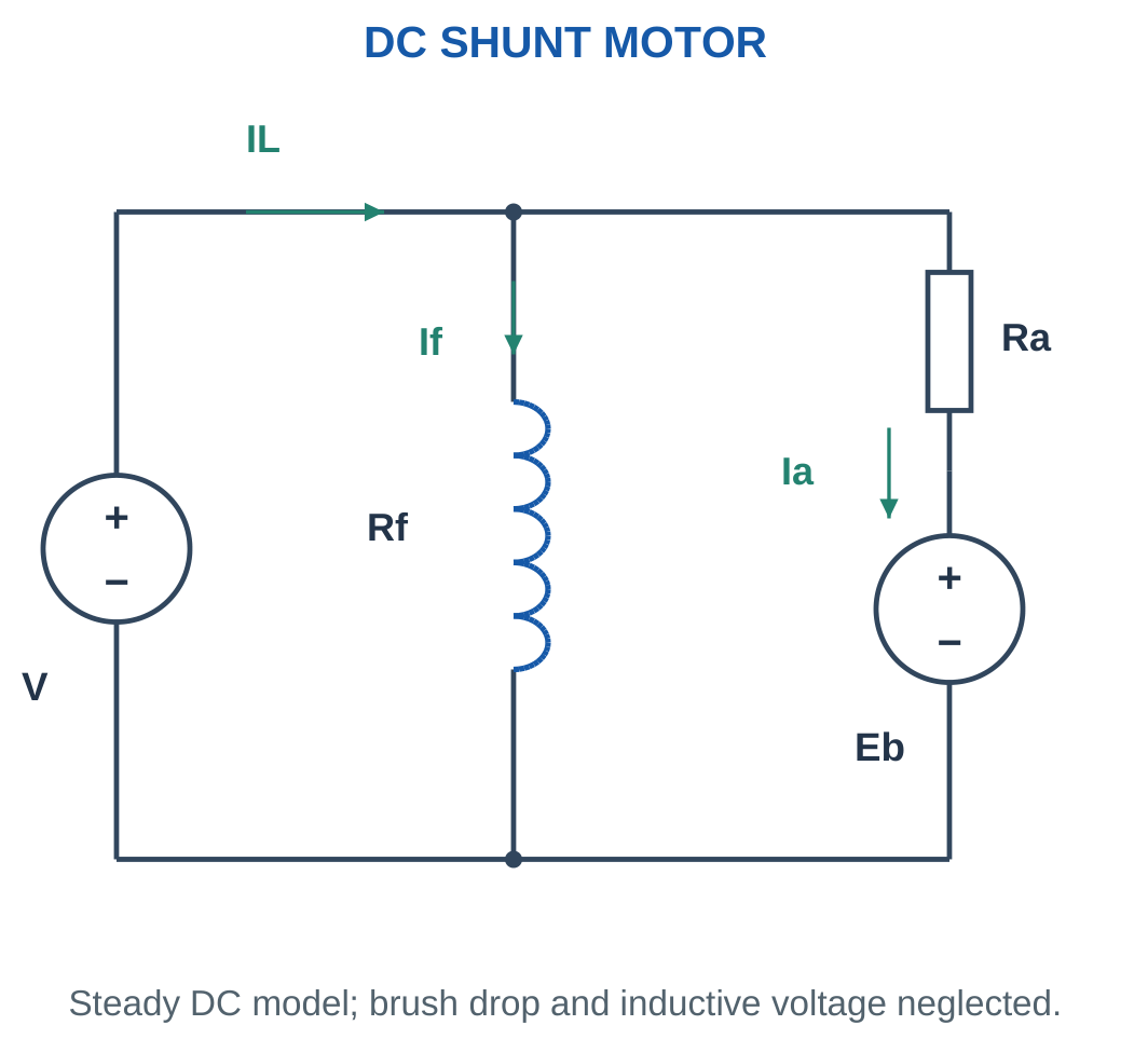
For a shunt motor:
IL = Ia + If
The field branch also consumes:
Pfield = VIf = If²Rf
Whole-motor input must include this branch power.

Efficiency
Useful shaft power equals developed power minus specified rotational and other downstream losses.
η = Pshaft/Pin
Both powers must use watts and the same system boundary.
For a shunt motor supplied from one source:
Pin = VIL
A separately supplied field requires a clear boundary. Include its input if whole-motor or whole-system efficiency is requested.
Common Efficiency Errors
Using armature current instead of line current omits field input in a shunt motor.
Subtracting field loss from an armature-only input and again from total input counts the same loss twice.
Use only supplied or explicitly represented losses. An unspecified motor does not have an assumed fixed efficiency simply because a familiar application is mentioned.
Worked Problem 5.16: Complete Shunt-Motor Power Balance

Problem: A shunt motor takes 25 A at 220 V. Field resistance is 110 Ω, armature resistance 0.5 Ω and rotational loss 250 W. Find Ia, Eb, output and efficiency.
Step 1: Calculate branch currents.
If = 220/110 = 2 A
Ia = 25 − 2 = 23 A
Step 2: Calculate back EMF and developed power.
Eb = 220 − 23 × 0.5 = 208.5 V
Pdev = 208.5 × 23 = 4795.5 W
Step 3: Calculate output and input.
Pshaft = 4795.5 − 250 = 4545.5 W
Pin = 220 × 25 = 5500 W
Step 4: Calculate efficiency.
η = 4545.5/5500 = 82.6455%
Loss check:
- Field loss = 440 W.
- Armature copper loss = 264.5 W.
- Rotational loss = 250 W.
- Total loss = 954.5 W.
Input equals 4545.5 + 954.5 = 5500 W.
Small DC Motor and Load

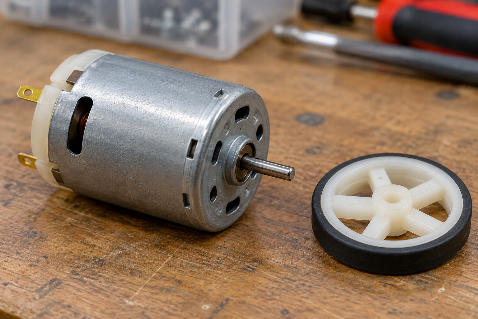
Starting or stalled current can differ greatly from running current. A driver must be assessed against the relevant state.
Electrical input, internal losses and useful shaft output remain separate parts of the power balance even in a small motor.
Worked Problem 5.17: Shunt Motor at 120 V
Problem: A shunt motor takes 15 A at 120 V. Field resistance is 120 Ω, armature resistance 0.8 Ω and rotational loss 100 W.
Step 1:
If = 120/120 = 1 A
Ia = 15 − 1 = 14 A
Step 2:
Eb = 120 − 14 × 0.8 = 108.8 V
Pdev = 108.8 × 14 = 1523.2 W
Step 3:
Pshaft = 1523.2 − 100 = 1423.2 W
Pin = 120 × 15 = 1800 W
Step 4:
η = 1423.2/1800 = 79.0667%
The loss check gives 120 W field loss, 156.8 W armature copper loss and 100 W rotational loss. Their total is 376.8 W, matching input minus output.
8. Starting Current and the Need for Control
At standstill, Eb is approximately zero.
Without added current control, the simplified armature current is:
Istart = V/Ra
Since armature resistance is small relative to voltage divided by normal current, this starting estimate can be much larger than rated current.

Textbook Resistance Model
A temporary series resistance can limit initial current in a basic analytical model.
For a permitted initial current Ilimit:
Rtotal = V/Ilimit
The additional resistance is:
Radd = V/Ilimit − Ra
The existing armature resistance is already included in the total.
The result is an analytical starting value. A complete starter design also needs duration, thermal rating, switching, inductance and protective information.
Electronic Current Control
Modern drives can limit current electronically. The controller still has to account for the machine’s electrical and thermal limits.
The resistance-only estimate must not be treated as a detailed instantaneous waveform. It identifies the current-limiting requirement under the stated approximation.
No-Load Series-Motor Caution
A DC series motor is not operated without its intended mechanical load unless its design and control explicitly prevent excessive speed.
Weak flux at low current can allow overspeed. This follows from the speed-flux relationship but remains a machine-use limitation rather than a numerical shortcut.
Worked Problem 5.18: Initial Current Limit
Problem: A stationary armature has Ra = 0.5 Ω and supply 220 V. Estimate uncontrolled current and added resistance for a 40 A initial limit.
Step 1:
Istart = 220/0.5 = 440 A
Step 2:
Rtotal = 220/40 = 5.5 Ω
Step 3:
Radd = 5.5 − 0.5 = 5 Ω
Step 4: Find initial added-resistor heating rate.
Padd = 40² × 5 = 8000 W
Duration and thermal/drive ratings would be required for a practical design. The calculated 5 Ω is additional resistance, not total resistance.
Worked Problem 5.19: Starting Resistance at 120 V
Problem: Ra = 0.8 Ω, supply is 120 V and the initial limit is 25 A.
Step 1:
Istart = 120/0.8 = 150 A
Step 2:
Rtotal = 120/25 = 4.8 Ω
Step 3:
Radd = 4.8 − 0.8 = 4 Ω
Step 4:
Padd = 25² × 4 = 2500 W
The model limits the specified initial current. As back EMF changes during acceleration, current and resistor heating also change.
Worked Problem 5.20: Starting Resistance at 240 V
Problem: Ra = 0.4 Ω, supply is 240 V and the initial limit is 50 A.
Step 1:
Istart = 240/0.4 = 600 A
Step 2:
Rtotal = 240/50 = 4.8 Ω
Step 3:
Radd = 4.8 − 0.4 = 4.4 Ω
Step 4:
Padd = 50² × 4.4 = 11000 W
The large initial heating rate illustrates why resistance value alone cannot establish a complete component specification.
9. DC Motor Speed-Control Concepts
For fixed machine geometry:
N ∝ (V − IaRa)/Φ
This suggests three basic control variables:
- Armature voltage.
- Armature-circuit resistance.
- Field flux.
Each changes speed together with current, torque and loss constraints.


Armature-Voltage Control
At approximately constant flux, lowering armature voltage reduces available back EMF and speed for a stated current condition.
The comparison should use V − IaRa, rather than terminal voltage alone, whenever resistance drop is included.
Armature-Resistance Control
Added armature series resistance increases voltage drop and heat loss. It tends to reduce speed under load.
This is not an efficient general substitute for a controlled supply because useful input is dissipated in the added resistance.
Field Weakening
Reducing flux can raise speed for a suitable voltage/current condition.
However:
Tdev ∝ ΦIa
so torque per ampere falls. The inverse-flux relationship does not promise unlimited speed or unchanged torque capability.
Complete Operating-Point Comparison
If current changes, recalculate back EMF at both points:
Eb1 = V1 − Ia1Ra
Eb2 = V2 − Ia2Ra
Then use:
N2/N1 = (Eb2/Eb1)(Φ1/Φ2)
A ratio problem must identify which quantities remain fixed.
Worked Problem 5.21: Voltage Reduction at Constant Flux
Problem: A motor runs at 1000 rpm with V1 = 220 V, Ia1 = 20 A and Ra = 0.5 Ω. At the second point V2 = 180 V, Ia2 = 20 A and flux is unchanged.
Step 1:
Eb1 = 220 − 20 × 0.5 = 210 V
Step 2:
Eb2 = 180 − 20 × 0.5 = 170 V
Step 3:
N2/N1 = 170/210
Step 4:
N2 = 1000 × 170/210 = 809.524 rpm
The lower armature voltage reduces speed under the supplied constant-current, constant-flux conditions.
Worked Problem 5.22: Field Reduction
Problem: A motor runs at 1200 rpm with V1 = 240 V, Ia1 = 25 A and Ra = 0.4 Ω. The second voltage and current are unchanged, but Φ2/Φ1 = 0.8.
Step 1:
Eb1 = 240 − 25 × 0.4 = 230 V
Step 2:
Eb2 = 230 V
Step 3:
N2/N1 = (230/230)/0.8 = 1.25
Step 4:
N2 = 1200 × 1.25 = 1500 rpm
Torque per ampere falls with the weaker field. This speed estimate does not establish an unrestricted operating condition.
Worked Problem 5.23: Changed Voltage and Current
Problem: A motor runs at 900 rpm with V1 = 200 V, Ia1 = 15 A and Ra = 0.6 Ω. At the second point V2 = 220 V, Ia2 = 20 A and flux is unchanged.
Step 1:
Eb1 = 200 − 15 × 0.6 = 191 V
Step 2:
Eb2 = 220 − 20 × 0.6 = 208 V
Step 3:
N2/N1 = 208/191
Step 4:
N2 = 900 × 208/191 = 980.105 rpm
Using terminal-voltage ratio alone would omit the changed resistance drop.
Worked Problem 5.24: Current and Flux Change
Problem: A motor runs at 1500 rpm with V1 = 120 V, Ia1 = 10 A and Ra = 0.8 Ω. At the second point V2 = 120 V, Ia2 = 12 A and Φ2/Φ1 = 0.9.
Step 1:
Eb1 = 120 − 10 × 0.8 = 112 V
Step 2:
Eb2 = 120 − 12 × 0.8 = 110.4 V
Step 3:
N2/N1 = (110.4/112)/0.9
Step 4:
N2 = 1642.86 rpm
Back EMF falls slightly, but flux also falls. The combined ratio predicts a speed increase. Both effects are required.
10. Types of DC Motors and Typical Applications
A separately excited motor has an independently supplied field.
A shunt motor has field and armature in parallel. A series motor has field and armature in series.
A compound motor combines shunt and series field effects. In cumulative compounding, their main field contributions aid.
A PMDC motor uses permanent magnets for its main field.

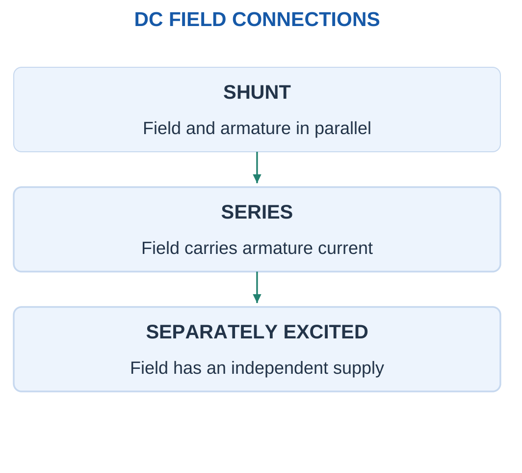
Comparison Table
| Type | Main qualitative behaviour | Example use context |
|---|---|---|
| Separately excited | Independent field and armature control | Controlled laboratory or industrial drives |
| Shunt | Approximately steady speed over a suitable load range | Machine tools and constant-speed duties |
| Series | High starting torque in the stated range | Classical traction and hoisting examples |
| Cumulative compound | Shunt excitation with an aiding series effect | Duties requiring starting torque and suitable speed behaviour |
| PMDC | Permanent magnets establish the main field | Small actuators and compact drives |
These are illustrative contexts. Motor selection also depends on duty, control, ratings, environment and maintenance.
Current Relationships
For the simple series connection:
IL = Ia = If
For a shunt motor:
IL = Ia + If
Use the actual connection before applying flux or torque comparisons.
Torque-Current Relationships
At constant flux:
T2/T1 = Ia2/Ia1
For an unsaturated series comparison:
T2/T1 = (Ia2/Ia1)²
Doubling current can therefore double torque under constant flux or approximately quadruple it under the unsaturated series assumption.
The difference comes from the flux model.
Worked Problem 5.25: Constant-Flux Torque Comparison
Problem: A motor develops 10 N·m at armature current 5 A. Estimate torque at 10 A with constant flux.
Step 1:
Current ratio = 10/5 = 2
Step 2: With unchanged flux, torque ratio equals current ratio.
T2/T1 = 2
Step 3:
T2 = 10 × 2 = 20 N·m
Step 4: Keep the supplied assumption.
The unsaturated series square law is not used because this problem states constant flux. The result concerns developed torque under that model.
Worked Problem 5.26: Unsaturated Series Torque
Problem: A motor develops 12 N·m at 8 A. Estimate torque at 12 A using an unsaturated series model.
Step 1:
Current ratio = 12/8 = 1.5
Step 2: Flux is proportional to current, so torque follows the square of current.
T2/T1 = 1.5² = 2.25
Step 3:
T2 = 12 × 2.25 = 27 N·m
Step 4: Recognise the saturation limitation.
If the series field saturates, flux no longer scales in the same proportion and the square-law estimate becomes unreliable.
Worked Problem 5.27: Another Series Torque Comparison
Problem: A motor develops 20 N·m at 10 A. Estimate torque at 15 A using an unsaturated series model.
Step 1:
Current ratio = 15/10 = 1.5
Step 2:
Torque ratio = 1.5² = 2.25
Step 3:
T2 = 20 × 2.25 = 45 N·m
Step 4: Compare the model choices.
A constant-flux assumption would give 30 N·m. The 45 N·m result depends on flux increasing with current in the stated unsaturated range.
11. BLDC Motor Construction and Operation
A brushless DC motor has a permanent-magnet rotor and stator windings supplied through an electronic drive.
It has no mechanical brush-and-commutator assembly performing armature commutation.
The drive switches stator currents according to rotor position and the chosen control method.

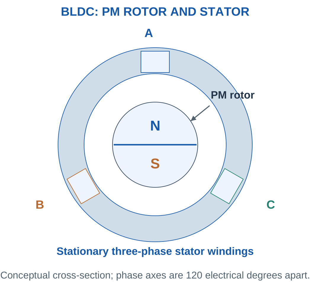
Meaning of BLDC
The name refers to the DC-fed drive system. Phase voltages and currents are electronically switched and vary with time.
Connecting DC indiscriminately across fixed phases does not provide continuous correct commutation.
The switching function has moved into electronics. Torque depends on coordinating stator excitation with rotor magnets.
Rotor Position
Position can be measured using devices such as Hall sensors or inferred through a suitable sensorless method.
Back-EMF-based inference is difficult at standstill because speed-dependent back EMF is absent. Practical drives need an appropriate startup strategy.
Brushless operation avoids brush wear but does not eliminate controller requirements.
Electrical Cycles
With P total rotor poles:
p = P/2
where p is pole-pair count.
At N rpm:
fe = pN/60
Typical applications include fans, pumps, compact motion systems and suitable vehicle auxiliaries. Exact motor and control choices depend on waveform, duty and controller design.
Worked Problem 5.28: Four-Pole BLDC Frequency
Problem: A four-pole BLDC rotor turns at 1500 rpm. Find mechanical rate, electrical frequency and ideal six-step interval rate.
Step 1:
Mechanical rate = 1500/60 = 25 revolutions/s
Step 2:
p = 4/2 = 2
Each mechanical revolution contains two electrical cycles.
Step 3:
fe = 2 × 25 = 50 Hz
Step 4:
Interval rate = 6fe = 300 intervals/s
Interval duration = 1/300 = 3.33333 ms
These are ideal commutation intervals, not an independently chosen PWM carrier frequency.
Brushless Motor Construction


A BLDC drive uses electronic commutation. Electrical cycles and mechanical revolutions depend on pole-pair count.
Current-torque relations require the specified model. The physical arrangement alone does not establish a numerical torque constant or current convention.
Worked Problem 5.29: Ten-Pole BLDC Frequency
Problem: A ten-pole rotor turns at 1200 rpm. Find mechanical rate, electrical frequency and six-step interval rate.
Step 1:
Mechanical rate = 1200/60 = 20 revolutions/s
Step 2:
p = 10/2 = 5
Step 3:
fe = 5 × 20 = 100 Hz
Step 4:
Interval rate = 6 × 100 = 600 intervals/s
Interval duration = 1/600 = 1.66667 ms
Although mechanical speed is lower than in the previous example, electrical frequency is higher because the rotor has more pole pairs.
12. Electronic Commutation and Electrical Frequency
One introductory BLDC method uses six current states per electrical cycle.
In each idealised state:
- One phase is driven positive.
- One phase is driven negative.
- One phase is floating.
The next state advances the stator excitation relative to the rotor.

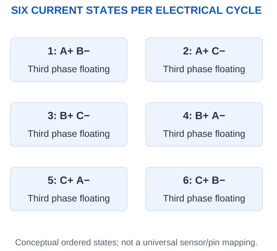
Example State Sequence
| State | Positive Phase | Negative Phase | Floating Phase |
|---|---|---|---|
| 1 | A | B | C |
| 2 | A | C | B |
| 3 | B | C | A |
| 4 | B | A | C |
| 5 | C | A | B |
| 6 | C | B | A |
Actual state-to-sensor mapping depends on winding, sensor and direction conventions.
The table is a consistent abstract sequence, not a universal connector-pin or Hall-code chart.
Frequency Relationships
fe = pN/60
For six intervals per electrical cycle:
Interval rate = 6fe
Interval duration = 1/(6fe)
Each mechanical revolution contains:
6p commutation intervals
A multi-pole rotor completes several electrical cycles during one mechanical revolution. Mechanical rpm is therefore different from electrical hertz.
Drive Blocks
A control block diagram separates the DC source, inverter, phase windings, rotor and position feedback.
This separation helps identify where electrical input is measured and how switching is coordinated. Detailed transistor design is beyond the introductory BLDC concept.
Worked Problem 5.30: Shaft Speed from Electrical Frequency
Problem: A six-step drive completes 150 electrical cycles per second for a six-pole rotor. Find shaft rpm, intervals per mechanical revolution and interval duration.
Step 1:
p = 6/2 = 3
Step 2:
N = 60fe/p = 60 × 150/3 = 3000 rpm
Step 3:
Intervals per mechanical revolution = 6p = 18
Step 4:
Interval duration = 1/(6 × 150)
Interval duration = 0.00111111 s = 1.11111 ms
The switching-to-sensor code still depends on the actual drive convention.
Worked Problem 5.31: Eight-Pole Rotor
Problem: A six-step drive completes 200 electrical cycles per second for an eight-pole rotor.
Step 1:
p = 8/2 = 4
Step 2:
N = 60 × 200/4 = 3000 rpm
Step 3:
Intervals per mechanical revolution = 6 × 4 = 24
Step 4:
Interval duration = 1/(6 × 200)
Interval duration = 0.000833333 s = 0.833333 ms
The shaft speed matches the previous example, but the electrical cycle frequency and interval count differ.
Worked Problem 5.32: Ten-Pole Rotor
Problem: A six-step drive completes 100 electrical cycles per second for a ten-pole rotor.
Step 1:
p = 10/2 = 5
Step 2:
N = 60 × 100/5 = 1200 rpm
Step 3:
Intervals per mechanical revolution = 6 × 5 = 30
Step 4:
Interval duration = 1/(6 × 100)
Interval duration = 0.00166667 s = 1.66667 ms
One electrical cycle contains six intervals, while one mechanical revolution contains thirty intervals for this rotor.
13. BLDC Performance Ideas and Application Comparison
BLDC systems avoid brush wear and permit controlled commutation. They require an electronic drive and appropriate rotor-position information.
Losses include winding copper, magnetic and mechanical losses. If the inverter lies within the chosen input boundary, its conduction and switching losses are also relevant.


Lumped Motor Model
A supplied simplified model may define:
Tdev = KtI
Eb = Keω
The meanings of current I and constants Kt and Ke must be stated.
A brushed-armature constant cannot automatically be applied to an unspecified three-phase winding-current or line-to-line back-EMF convention.
Units of Constants
A Ke supplied in volts per rad/s requires angular speed in rad/s.
A constant supplied per 1000 rpm is a different numerical convention and must be used with the stated speed scale.
Converting units after an inconsistent substitution does not generally repair the physical model.
Output and Efficiency
Useful output remains:
Pshaft = Tshaftω
If the model gives developed torque:
Pdev = Tdevω
Subtract specified rotational losses to obtain shaft output.
Motor-only efficiency and drive-plus-motor efficiency can differ because their input boundaries differ.
Comparing Motor Types
A useful comparison with brushed DC mentions:
- Switching method.
- Rotor field arrangement.
- Maintenance.
- Controller requirements.
- Position information.
- Input-output boundary.
Brushless construction alone does not prove a particular efficiency value. Numerical comparison requires measured or supplied powers and losses.
Worked Problem 5.33: Supplied BLDC Torque Model
Problem: Kt = 0.15 N·m/A and model current is 4 A. At 3000 rpm, rotational loss is 12 W. Find developed torque, developed power and shaft output.
Step 1:
Tdev = 0.15 × 4 = 0.6 N·m
Step 2:
ω = 2π × 3000/60 = 314.159 rad/s
Step 3:
Pdev = 0.6 × 314.159 = 188.496 W
Step 4:
Pshaft = 188.496 − 12 = 176.496 W
Electrical input would require the relevant electrical losses or efficiency boundary.
Worked Problem 5.34: BLDC Output at 1500 rpm
Problem: Kt = 0.2 N·m/A, model current is 5 A, speed is 1500 rpm and rotational loss is 15 W.
Step 1:
Tdev = 0.2 × 5 = 1 N·m
Step 2:
ω = 157.08 rad/s
Step 3:
Pdev = 1 × 157.08 = 157.08 W
Step 4:
Pshaft = 157.08 − 15 = 142.08 W
The loss is subtracted from power. An equivalent loss torque would require dividing the loss power by angular speed.
Worked Problem 5.35: BLDC Output at 2400 rpm
Problem: Kt = 0.08 N·m/A, model current is 6 A, speed is 2400 rpm and rotational loss is 8 W.
Step 1:
Tdev = 0.08 × 6 = 0.48 N·m
Step 2:
ω = 251.327 rad/s
Step 3:
Pdev = 0.48 × 251.327 = 120.637 W
Step 4:
Pshaft = 120.637 − 8 = 112.637 W
The calculation uses the current definition supplied by the lumped model. It does not infer a different phase-current convention.
14. Three-Phase Induction Motor Construction
A three-phase induction motor has a stator carrying distributed phase windings and a rotor in which currents are induced by relative field motion.
A squirrel-cage rotor uses conducting bars connected by end rings.


Stator Function
The stator receives three-phase electrical input. Its winding arrangement produces the rotating magnetic field.
The magnetic circuit and distributed winding allow the spatial field to progress around the machine.
Rotor Function
The cage is not normally connected to an external electrical supply. Stator field motion relative to rotor conductors induces rotor EMF and current.
A wound-rotor machine uses a wound rotor instead, but the basic induction principle still relies on relative motion.
Construction Features
Laminated cores reduce eddy-current paths. Bearings, shaft and cooling arrangements support mechanical operation.
There is no ordinary mechanical commutator reversing cage-rotor currents as in a brushed DC machine.
No Rotor Supply Does Not Mean No Rotor Current
A rotor can carry substantial induced currents without a wired external supply.
These currents produce torque and rotor copper loss. Their frequency depends on slip rather than always equalling stator supply frequency.
Three-phase induction motors are used in pump, fan, conveyor and compressor duties. Selection still requires load, starting method, supply, rating and environmental information.
15. Rotating Magnetic Field
Three balanced stator currents in windings displaced by 120 electrical degrees produce a resultant rotating magnetic field.
In the ideal sinusoidal distributed-winding model, the resultant has constant amplitude and continuously changing angular position.

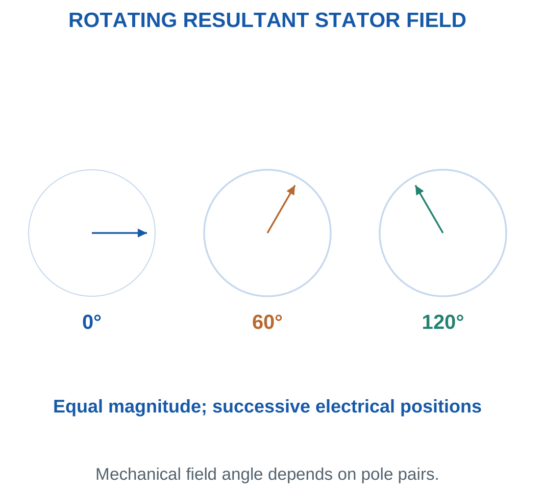
Synchronous Field Speed
The mechanical field speed is:
Ns = 120f/P rpm
where f is supply frequency and P is total pole count.
More poles at the same frequency give a lower mechanical field speed.
Using pole pairs p:
Ns = 60f/p
Electrical phase progression and mechanical field rotation are related through this count.
Direction
Phase sequence determines field-rotation direction.
Reversing the conceptual sequence reverses field rotation. This explains direction control without requiring any live connection change during a laboratory exercise.
Constant Magnitude and Changing Direction
A rotating resultant differs from a single pulsating field.
At a fixed stator point, the field changes with time even though the ideal resultant vector maintains constant amplitude as it rotates.
The familiar 1.5 resultant-amplitude factor follows from an ideal balanced sinusoidal winding-space model. Real winding distributions and harmonics require additional factors.
Worked Problem 5.36: Rotor Speed from Slip
Problem: A 50 Hz field has four poles. Rotor slip is 3%. Find field speed, rotor speed, relative speed and electrical cycles per mechanical field revolution.
Step 1:
Ns = 120 × 50/4 = 1500 rpm
Step 2:
s = 3/100 = 0.03
N = 1500(1 − 0.03) = 1455 rpm
Step 3:
Relative speed = sNs = 45 rpm
Step 4:
Electrical cycles per mechanical field revolution = P/2 = 2
Pole-pair count and slip describe different relationships. Neither should replace the other in the calculation.
Industrial Induction Motor


Rotor speed is compared with rotating-field synchronous speed. Slip is a ratio, rather than a fixed universal rpm difference.
Electrical input differs from shaft output through losses. Actual slip and efficiency must come from supplied operating data or a suitable model.
Worked Problem 5.37: Six Poles at 60 Hz
Problem: A balanced 60 Hz stator field has six poles. Rotor slip is 2.5%.
Step 1:
Ns = 120 × 60/6 = 1200 rpm
Step 2:
s = 0.025
N = 1200 × 0.975 = 1170 rpm
Step 3:
Relative speed = 0.025 × 1200 = 30 rpm
Step 4:
Pole pairs = 6/2 = 3
Each mechanical field revolution contains three electrical cycles. The 30 rpm difference is a separate rotor-slip quantity.
16. Synchronous Speed and Pole Count
Each pair of stator poles corresponds to one electrical cycle per mechanical field revolution.
With p pole pairs:
Ns = 60f/p
With P total poles:
Ns = 120f/P
Pole count is an even integer in the elementary model.


Common 50 Hz Values
| Poles | Pole Pairs | Synchronous Speed |
|---|---|---|
| 2 | 1 | 3000 rpm |
| 4 | 2 | 1500 rpm |
| 6 | 3 | 1000 rpm |
| 8 | 4 | 750 rpm |
These are field speeds. A loaded induction rotor normally runs slightly below the associated field speed during motoring.
Inferring Pole Count
Measured rotor speed cannot simply replace synchronous speed in:
P = 120f/Ns
Doing so can produce a noninteger pole count.
Use the nearby synchronous speed above the measured motoring speed together with the supplied slip condition or operating information.
Variable Frequency
For fixed poles, changing frequency changes synchronous speed.
A practical drive must also manage voltage, flux, current and mechanical limits. The speed equation alone does not establish the complete operating envelope.
Worked Problem 5.38: Two Poles at 50 Hz
Problem: A stator has two poles and frequency 50 Hz. Find field speed in rpm and rad/s.
Step 1:
p = 1
Field revolutions per second = 50
Step 2:
Ns = 120 × 50/2 = 3000 rpm
Step 3:
ωs = 2π × 3000/60 = 314.159 rad/s
Step 4: Interpret the result.
A normally loaded motoring rotor runs below this field speed. Without slip, exact rotor speed is not determined.
Worked Problem 5.39: Four Poles at 50 Hz
Problem: A stator has four poles and frequency 50 Hz.
Step 1:
p = 2
Field revolutions per second = 50/2 = 25
Step 2:
Ns = 120 × 50/4 = 1500 rpm
Step 3:
ωs = 157.08 rad/s
Step 4: Keep the quantities separate.
The field speed is 1500 rpm. Actual loaded rotor speed requires slip information and is normally lower.
Worked Problem 5.40: Six Poles at 50 Hz
Problem: A stator has six poles and frequency 50 Hz.
Step 1:
p = 3
Field revolutions per second = 50/3 = 16.6667
Step 2:
Ns = 120 × 50/6 = 1000 rpm
Step 3:
ωs = 104.72 rad/s
Step 4: Interpret the pole effect.
Increasing poles from four to six lowers field speed at the same supply frequency. The equation describes the field rather than a guaranteed loaded rotor speed.
Worked Problem 5.41: Four Poles at 60 Hz
Problem: A stator has four poles and frequency 60 Hz.
Step 1:
p = 2
Field revolutions per second = 60/2 = 30
Step 2:
Ns = 120 × 60/4 = 1800 rpm
Step 3:
ωs = 188.496 rad/s
Step 4: Compare frequency conditions.
The same pole count gives higher synchronous speed at higher supply frequency. Exact loaded rotor speed still requires slip.
17. Slip and Rotor Speed
Slip is the fractional difference between synchronous field speed and rotor speed:
s = (Ns − N)/Ns
Percentage slip is:
100s
Rearranging:
N = Ns(1 − s)


Limiting Conditions
At standstill:
N = 0, s = 1
At synchronous speed:
N = Ns, s = 0
For elementary normal motoring:
0 < s < 1
Positive slip provides the relative motion required for induced rotor current and torque.
At exactly synchronous speed, the ideal steady rotor sees no changing field due to relative motion. It cannot sustain nonzero load torque from the elementary induction mechanism.
Percentage Conversion
A slip of 4% means:
s = 0.04
It does not mean s = 4.
Substituting 4 into N = Ns(1 − s) produces an inappropriate negative speed for the stated normal-motoring problem.
Load Response
Within the stable operating region, increased load slows the rotor slightly. Slip rises and permits greater induced current and torque.
The small-slip trend cannot be extended indefinitely because the full torque characteristic has a maximum.
Worked Problem 5.42: Slip and Rotor Frequency


Problem: A four-pole motor on 50 Hz runs at 1440 rpm. Find synchronous speed, slip, relative speed and rotor frequency.
Step 1:
Ns = 120 × 50/4 = 1500 rpm
Relative speed = 1500 − 1440 = 60 rpm
Step 2:
s = 60/1500 = 0.04 = 4%
Step 3:
fr = sf = 0.04 × 50 = 2 Hz
Step 4:
N = 1500 × 0.96 = 1440 rpm
Rotor current frequency is different from shaft revolutions per second.
Worked Problem 5.43: Six-Pole Motor Slip
Problem: A six-pole motor on 50 Hz runs at 960 rpm.
Step 1:
Ns = 1000 rpm
Relative speed = 1000 − 960 = 40 rpm
Step 2:
s = 40/1000 = 0.04 = 4%
Step 3:
fr = 0.04 × 50 = 2 Hz
Step 4:
N = 1000 × 0.96 = 960 rpm
This motor has the same fractional slip and rotor frequency as the previous example, although its rpm difference is smaller.
Worked Problem 5.44: Slip at 60 Hz
Problem: A four-pole motor on 60 Hz runs at 1746 rpm.
Step 1:
Ns = 1800 rpm
Relative speed = 1800 − 1746 = 54 rpm
Step 2:
s = 54/1800 = 0.03 = 3%
Step 3:
fr = 0.03 × 60 = 1.8 Hz
Step 4:
N = 1800 × 0.97 = 1746 rpm
A slip of 3% does not itself mean a rotor frequency of 3 Hz. Supply frequency must also be included.
Worked Problem 5.45: Eight-Pole Motor Slip
Problem: An eight-pole motor on 50 Hz runs at 720 rpm.
Step 1:
Ns = 750 rpm
Relative speed = 750 − 720 = 30 rpm
Step 2:
s = 30/750 = 0.04 = 4%
Step 3:
fr = 0.04 × 50 = 2 Hz
Step 4:
N = 750 × 0.96 = 720 rpm
Slip is a ratio. The same ratio can occur at several different synchronous and rotor speeds.
18. Rotor Frequency and Induced EMF
Rotor current frequency is:
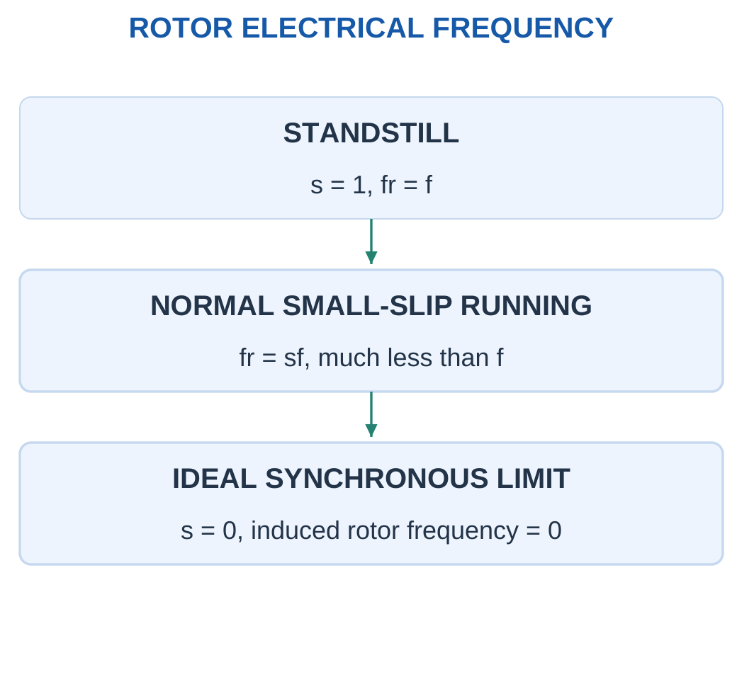
fr = sf
At standstill, s = 1 and rotor frequency equals stator supply frequency.
During normal small-slip running, rotor electrical frequency is much lower.

Running Rotor EMF
If standstill induced rotor EMF per phase is E20 and main flux is treated as constant:
E2s = sE20
The lower relative speed during running reduces induced EMF.
Running Rotor Reactance
Leakage reactance depends on rotor frequency. With fixed leakage inductance:
X2s = sX20
where X20 is the standstill rotor reactance.
Distinct Frequencies and Speeds
A rotor near 1500 rpm can have rotor current frequency of only a few hertz. Its shaft speed and rotor electrical frequency describe different processes.
Use the same fractional s in fr, E2s and X2s. Do not multiply by 100 after a percentage has already been converted.
The scaling assumes maintained main flux and the stated equivalent-parameter model.
Worked Problem 5.46: Running Rotor Quantities
Problem: A four-pole motor on 50 Hz operates at s = 0.04. E20 = 100 V per phase and X20 = 2 Ω.
Step 1:
Ns = 1500 rpm
N = 1500 × 0.96 = 1440 rpm
Step 2:
fr = 0.04 × 50 = 2 Hz
Step 3:
E2s = 0.04 × 100 = 4 V per phase
Step 4:
X2s = 0.04 × 2 = 0.08 Ω
At standstill, s = 1 and the values recover E20 and X20.
Worked Problem 5.47: Running Quantities at 60 Hz
Problem: A four-pole motor on 60 Hz has s = 0.03, E20 = 120 V per phase and X20 = 3 Ω.
Step 1:
Ns = 1800 rpm
N = 1800 × 0.97 = 1746 rpm
Step 2:
fr = 0.03 × 60 = 1.8 Hz
Step 3:
E2s = 0.03 × 120 = 3.6 V per phase
Step 4:
X2s = 0.03 × 3 = 0.09 Ω
Both the induced EMF and frequency-dependent reactance are scaled by the same slip fraction.
Worked Problem 5.48: Six-Pole Running Quantities
Problem: A six-pole motor on 50 Hz has s = 0.05, E20 = 80 V per phase and X20 = 1.5 Ω.
Step 1:
Ns = 1000 rpm
N = 1000 × 0.95 = 950 rpm
Step 2:
fr = 0.05 × 50 = 2.5 Hz
Step 3:
E2s = 0.05 × 80 = 4 V per phase
Step 4:
X2s = 0.05 × 1.5 = 0.075 Ω
The model gives a running EMF of 4 V per phase, while the standstill value is 80 V per phase.
Worked Problem 5.49: Standstill Check
Problem: A four-pole motor on 50 Hz has s = 1, E20 = 100 V per phase and X20 = 2 Ω.
Step 1:
Ns = 1500 rpm
N = 1500(1 − 1) = 0 rpm
Step 2:
fr = 1 × 50 = 50 Hz
Step 3:
E2s = 1 × 100 = 100 V per phase
Step 4:
X2s = 1 × 2 = 2 Ω
The limiting case confirms the meaning of the standstill parameters.
19. Induction-Motor Torque and Power Conversion
Rotor induced currents interact with the rotating magnetic field and produce electromagnetic torque.
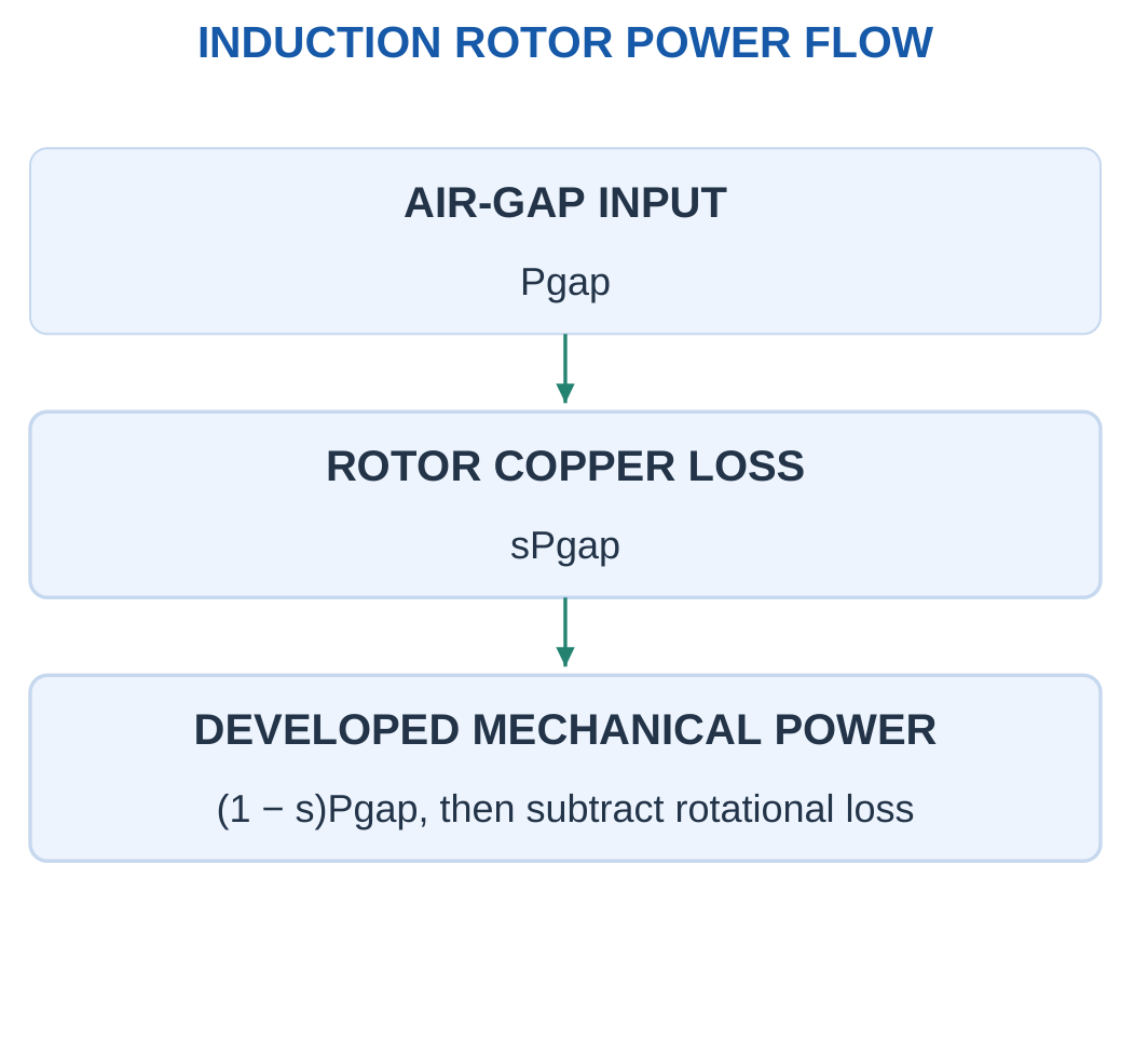
Let Pgap be the power transferred across the air gap into the rotor.
In the simple steady model:
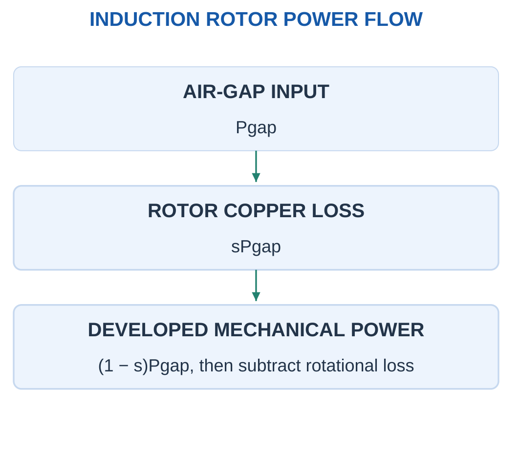
Pcu,rotor = sPgap
Pdev = (1 − s)Pgap

Developed Torque
For nonzero rotor speed:
Tdev = Pdev/ωr
Since:
ωr = (1 − s)ωs
the same torque is:
Tdev = Pgap/ωs
This second expression provides an independent check and helps interpret finite starting torque.
Shaft Output
With rotational loss Prot:
Pshaft = Pdev − Prot
Tshaft = Pshaft/ωr
Shaft torque is smaller than developed torque when rotational losses are present.
Torque-Slip Curve
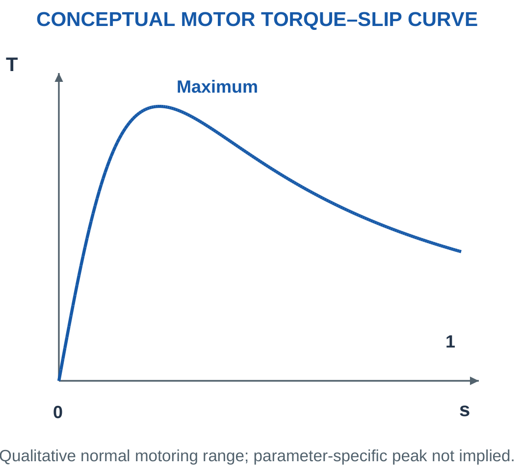
At small slip under a fixed-frequency, maintained-flux model, torque initially rises approximately with slip.
The full characteristic reaches a maximum and does not rise indefinitely.

Torque and Power at Standstill
At standstill, mechanical power Tω is zero because ω is zero. Electromagnetic torque can still be finite.
At s = 1:
Pcu,rotor = Pgap
Pdev = 0
Rotor input can therefore be dissipated as copper heat in this simplified split. A motor can draw power and produce torque without useful shaft motion.
Worked Problem 5.50: Power Split and Both Torques

Problem: A four-pole motor on 50 Hz has s = 0.04, Pgap = 10000 W and rotational loss 300 W.
Step 1:
Ns = 1500 rpm
N = 1440 rpm
ωr = 150.796 rad/s
Step 2:
Pcu,rotor = 0.04 × 10000 = 400 W
Pdev = 0.96 × 10000 = 9600 W
Step 3:
Pshaft = 9600 − 300 = 9300 W
Tdev = 9600/150.796 = 63.662 N·m
Step 4:
Tdev = Pgap/ωs = 10000/157.08 = 63.662 N·m
Tshaft = 9300/150.796 = 61.6725 N·m
The two developed-torque calculations agree.
Worked Problem 5.51: Six-Pole Motor Power Flow
Problem: A six-pole motor on 50 Hz has s = 0.05, Pgap = 6000 W and rotational loss 200 W.
Step 1:
Ns = 1000 rpm
N = 950 rpm
ωr = 99.4838 rad/s
Step 2:
Pcu,rotor = 0.05 × 6000 = 300 W
Pdev = 0.95 × 6000 = 5700 W
Step 3:
Pshaft = 5700 − 200 = 5500 W
Tdev = 5700/99.4838 = 57.2958 N·m
Step 4:
Tdev = 6000/104.72 = 57.2958 N·m
Tshaft = 5500/99.4838 = 55.2854 N·m
The synchronous angular speed is paired with air-gap power, while rotor angular speed is paired with developed mechanical power.
Worked Problem 5.52: Power Flow at 60 Hz
Problem: A four-pole motor on 60 Hz has s = 0.03, Pgap = 12000 W and rotational loss 400 W.
Step 1:
Ns = 1800 rpm
N = 1746 rpm
ωr = 182.841 rad/s
Step 2:
Pcu,rotor = 0.03 × 12000 = 360 W
Pdev = 0.97 × 12000 = 11640 W
Step 3:
Pshaft = 11640 − 400 = 11240 W
Tdev = 11640/182.841 = 63.662 N·m
Step 4:
Tdev = 12000/188.496 = 63.662 N·m
Tshaft = 11240/182.841 = 61.4743 N·m
The supplied rotational loss accounts for the difference between developed and shaft torque.
Worked Problem 5.53: Higher-Slip Power Flow
Problem: A four-pole motor on 50 Hz has s = 0.08, Pgap = 8000 W and rotational loss 250 W.
Step 1:
Ns = 1500 rpm
N = 1380 rpm
ωr = 144.513 rad/s
Step 2:
Pcu,rotor = 0.08 × 8000 = 640 W
Pdev = 0.92 × 8000 = 7360 W
Step 3:
Pshaft = 7360 − 250 = 7110 W
Tdev = 7360/144.513 = 50.9296 N·m
Step 4:
Tdev = 8000/157.08 = 50.9296 N·m
Tshaft = 7110/144.513 = 49.1996 N·m
A greater slip fraction gives a greater rotor copper-loss fraction in the stated model.
20. Induction-Motor Applications and Operating Choices
Three-phase induction motors suit many industrial loads because cage construction is robust and does not require a mechanical commutator.
Pumps, fans, compressors and conveyors are familiar contexts. Final motor and drive choice depends on the actual duty.


Load Behaviour
A fan or centrifugal-pump load can have torque that rises strongly with speed. A conveyor may require substantial starting torque.
These differences matter, but a numerical torque law should only be used when supplied by the problem.
An application name alone is not enough to infer every load parameter.
Electrical Input and Line Current
For shaft output Pshaft and efficiency η:
Pin = Pshaft/η
For balanced three-phase input:
Pin = √3VLIL PF
Therefore:
IL = Pin/(√3VL PF)
Efficiency connects shaft watts to input watts. Power factor connects input watts to input apparent power.
Interpreting Ratings
A mechanical output rating in kW is not automatically electrical input kW.
A variable-frequency drive controls synchronous speed through frequency and manages voltage/current according to its strategy. The introductory speed relation is not a complete converter or protection design.
Worked Problem 5.54: Line Current for a Shaft Duty
Problem: A balanced motor delivers 7.5 kW at efficiency 0.9 and input PF 0.8. Supply is 400 V line-to-line RMS.
Step 1:
Pshaft = 7500 W
Pin = 7500/0.9 = 8333.33 W
Step 2:
S = Pin/PF = 8333.33/0.8 = 10416.7 VA
Step 3:
IL = 8333.33/(√3 × 400 × 0.8) = 15.0352 A
Step 4:
Ploss = 8333.33 − 7500 = 833.333 W
The data give total loss but do not divide it into individual components.
Worked Problem 5.55: Four-Kilowatt Shaft Duty
Problem: Shaft output is 4 kW, efficiency 0.85, PF 0.75 and line voltage 415 V RMS.
Step 1:
Pin = 4000/0.85 = 4705.88 W
Step 2:
S = 4705.88/0.75 = 6274.51 VA
Step 3:
IL = 4705.88/(√3 × 415 × 0.75) = 8.72913 A
Step 4:
Ploss = 4705.88 − 4000 = 705.882 W
Using 4000 W directly as electrical input would underestimate line current.
Worked Problem 5.56: Fifteen-Kilowatt Shaft Duty
Problem: A motor delivers 15 kW at efficiency 0.92 and PF 0.86 from a 440 V line supply.
Step 1:
Pin = 15000/0.92 = 16304.3 W
Step 2:
S = 16304.3/0.86 = 18958.5 VA
Step 3:
IL = 16304.3/(√3 × 440 × 0.86) = 24.8766 A
Step 4:
Ploss = 16304.3 − 15000 = 1304.35 W
The efficiency and power-factor factors are both needed because the calculation crosses two different relationships.
21. Solar Photovoltaic Systems: Cells to Useful Power
A photovoltaic cell converts absorbed light energy into electrical energy through the photovoltaic effect.
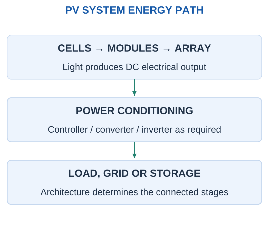
A module contains interconnected cells. Several modules form an array.
The electrical output is DC and varies with operating voltage, irradiance and cell temperature.

System Components
A system may contain:
- Mounting.
- DC wiring.
- Protection and isolation equipment.
- A controller or DC–DC stage.
- Storage when needed.
- An inverter for AC loads or grid interaction.
- The connected load or grid interface.
Batteries are not compulsory in every PV architecture. Stand-alone and grid-connected systems can have different needs.
Incident Power and Conversion Efficiency
For irradiance G and illuminated area A:
Pincident = GA
With G in W/m² and A in m², the result is watts.
At a specified point:
ηPV = Pout/(GA)
Use the area and conditions supplied by the question.
Irradiance and Energy
Irradiance is instantaneous power per area. Energy over time requires integration or an explicitly stated equivalent duration.
A module’s watt rating does not determine daily energy by itself.
PV production uses light, not simply panel heating. Higher cell temperature often reduces voltage and maximum power for a typical silicon module at fixed irradiance.
Worked Problem 5.57: Conversion from Incident Sunlight
Problem: A module has area 1.6 m², receives 1000 W/m² and delivers 320 W electrical output.
Step 1:
Pincident = 1000 × 1.6 = 1600 W
Step 2:
ηPV = 320/1600 = 0.2
Step 3:
ηPV = 20%
Step 4: Interpret the result.
This is an instantaneous operating-point efficiency. Daily energy additionally requires an output-time or irradiance-time model.
Worked Problem 5.58: Efficiency at Lower Irradiance
Problem: A 2 m² module receives 800 W/m² and delivers 280 W.
Step 1:
Pincident = 800 × 2 = 1600 W
Step 2:
ηPV = 280/1600 = 0.175
Step 3:
ηPV = 17.5%
Step 4: Keep the powers distinct.
The incident 1600 W is optical power. The useful output is the supplied 280 W electrical power.
Photovoltaic Module in Service


A module converts incident radiation under its operating conditions. Output depends on irradiance, temperature and operating point.
Area and sunlight alone do not specify useful delivered power without a model or conversion data.
22. Single-Diode PV Equivalent Circuit
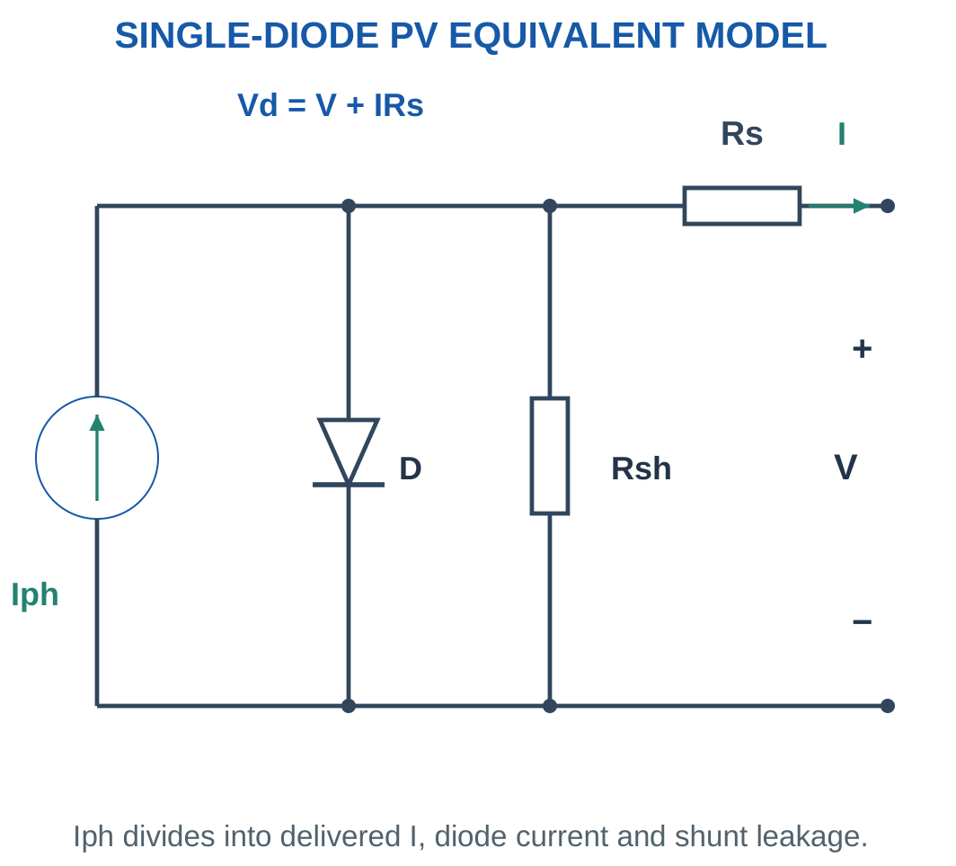
The single-diode model uses a light-generated current source Iph in parallel with a diode and shunt resistance Rsh.
Series resistance Rs is included at the output.
This is an equivalent electrical model, not a physical drawing of semiconductor layers.

General Current Equation
With delivered output current positive toward the load:
Vd = V + IRs
The model equation is:
I = Iph − I0[exp((V + IRs)/a) − 1] − (V + IRs)/Rsh
I0 is saturation current and a is the exponential voltage scale.
For a single cell:
a = nkBT/q
For an equivalent module of identical series cells under uniform conditions, the scale includes series-cell count:
a = nNs kBT/q
The other parameters must also correspond to the chosen module level.
Consistent Model Level
Do not insert a single-cell thermal-voltage scale into a whole-module equation while omitting series-cell count.
Examples either supply a directly or identify the cell model.
Larger Rs tends to reduce useful voltage and fill factor. Smaller Rsh increases internal leakage.
Simplified Model
With Rs = 0 and negligible shunt leakage:
I = Iph − I0[exp(V/a) − 1]
The following problems use this explicit simplified equation.
Worked Problem 5.59: Current from the Diode Equation


Problem: A cell model has Iph = 5 A, I0 = 10⁻⁸ A and a = 0.04 V. Neglect Rs and shunt leakage. Find output current and power at 0.6 V, plus Voc.
Step 1:
V/a = 0.6/0.04 = 15
I = 5 − 10⁻⁸[exp(15) − 1]
Step 2:
Idiode = 0.0326902 A
I = 4.96731 A
Step 3:
P = 0.6 × 4.96731 = 2.98039 W
Step 4: Set I = 0 at open circuit.
Voc = a ln(1 + Iph/I0)
Voc = 0.801205 V
The supplied generating voltage is below the open-circuit endpoint.
Worked Problem 5.60: Current at 0.7 V
Problem: Iph = 6 A, I0 = 2 × 10⁻⁸ A and a = 0.05 V. Find current, power and Voc for the simplified model at 0.7 V.
Step 1:
V/a = 14
Step 2:
Idiode = 2 × 10⁻⁸[exp(14) − 1] = 0.0240521 A
I = 6 − 0.0240521 = 5.97595 A
Step 3:
P = 0.7 × 5.97595 = 4.18316 W
Step 4:
Voc = 0.05 ln(1 + 6/(2 × 10⁻⁸)) = 0.975965 V
The current and voltage used for power are simultaneous operating values.
Worked Problem 5.61: Current at 0.55 V
Problem: Iph = 4 A, I0 = 10⁻⁷ A, a = 0.045 V and V = 0.55 V.
Step 1:
V/a = 0.55/0.045 = 12.2222
Step 2:
Idiode = 10⁻⁷[exp(12.2222) − 1] = 0.0203255 A
I = 3.97967 A
Step 3:
P = 0.55 × 3.97967 = 2.18882 W
Step 4:
Voc = 0.045 ln(1 + 4/10⁻⁷) = 0.787698 V
The exponential argument is dimensionless. Its voltage scale must belong to the same cell or module model as the terminal voltage.
23. Short Circuit, Open Circuit and the Current–Voltage Curve
The I–V curve shows current versus output voltage under specified conditions.
Short-circuit current Isc occurs at V = 0.
Open-circuit voltage Voc occurs at I = 0.
Neither endpoint delivers useful terminal power because P = VI is zero at each.


Simplified Endpoints
For Rs = 0 and effectively infinite Rsh:
I(V) = Iph − I0[exp(V/a) − 1]
At short circuit:
Isc = Iph
At open circuit:
Voc = a ln(1 + Iph/I0)
These endpoint formulae depend on the stated simplifications.
Curve Shape
The relatively flat current region changes into a knee near the high-voltage end.
A PV source is not an ideal constant-voltage source for every load, nor an ideal current source at every voltage.
The actual operating point depends on the connected load or converter condition.
Endpoint Multiplication
VocIsc is a useful bounding rectangle for fill factor. It is not a delivered operating power because its two factors occur at different points.
Similarly, Voc/Isc is not a fixed internal resistance that reproduces the entire nonlinear curve.
PV Electrical-Characteristic Test


Open circuit and short circuit are endpoints rather than maximum-power conditions.
An I–V curve and operating point are required to determine delivered power. Endpoint values cannot be multiplied as though they occur simultaneously.
Worked Problem 5.62: Endpoint Currents, Voltages and Power
Problem: Iph = 6 A, I0 = 2 × 10⁻⁸ A and a = 0.05 V. Use Rs = 0 and infinite Rsh.
Step 1: At V = 0, the diode term vanishes.
Isc = 6 A
Step 2:
Voc = 0.05 ln(1 + 6/(2 × 10⁻⁸))
Voc = 0.975965 V
Step 3:
Pshort = 0 × 6 = 0 W
Popen = 0.975965 × 0 = 0 W
Step 4:
VocIsc = 5.85579 W
This rectangle is not delivered power at either endpoint. Positive maximum power occurs at an intermediate simultaneous voltage-current pair.
Worked Problem 5.63: Another Endpoint Model
Problem: Iph = 4 A, I0 = 10⁻⁷ A and a = 0.045 V.
Step 1:
Isc = 4 A
Step 2:
Voc = 0.045 ln(1 + 4/10⁻⁷) = 0.787698 V
Step 3:
Pshort = 0 W
Popen = 0 W
Step 4:
VocIsc = 0.787698 × 4 = 3.15079 W
The product helps normalise the curve through fill factor. It does not represent an operating point at which both endpoint values are available together.
24. Power–Voltage Curve, Maximum-Power Point and Fill Factor
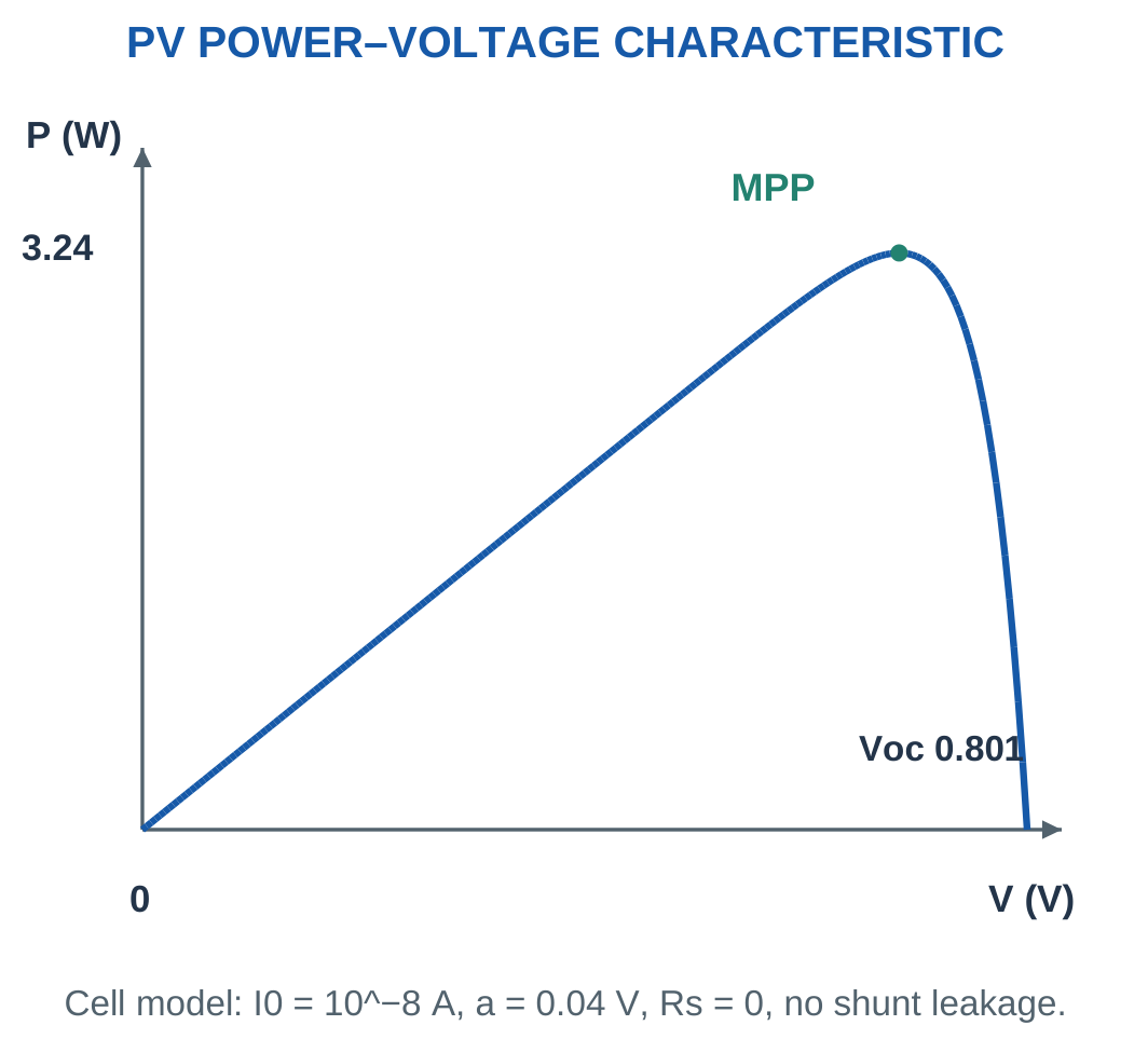
The P–V curve is obtained from:
P(V) = VI(V)
Power starts at zero at short circuit, rises to a maximum and returns to zero at open circuit.
The maximum-power point is the simultaneous pair Vmp and Imp:
Pmp = VmpImp

Fill Factor
FF = Pmp/(VocIsc)
Fill factor is dimensionless and below one for the ordinary generating curves considered here.
A larger value means the characteristic uses more of the endpoint rectangle.
It is not conversion efficiency. Efficiency instead compares electrical output with optical input GA.
Maximum-Power Tracking
Maximum-power tracking changes the electrical operating condition so that the source remains near its available maximum as conditions change.
It differs from moving a panel physically to track the sun. A system may use both techniques.
Mathematical MPP Condition
Since P = VI:
dP/dV = I + V(dI/dV)
At an interior maximum:
I + V(dI/dV) = 0
The examples use this condition or supplied measured operating points. MPP is not assumed to be one fixed percentage of Voc for every model.
Worked Problem 5.64: Fill Factor and Matching Resistance
Problem: A module has Voc = 40 V, Isc = 10 A and MPP at Vmp = 32 V, Imp = 9 A.
Step 1:
Pmp = 32 × 9 = 288 W
Step 2:
VocIsc = 40 × 10 = 400 W
FF = 288/400 = 0.72
Step 3:
Rload = Vmp/Imp = 32/9 = 3.55556 Ω
Step 4: Interpret the load.
The resistance matches this supplied operating point. At changed irradiance or temperature, the maximum-power point can move.
Worked Problem 5.65: Smaller Module Fill Factor
Problem: Voc = 22 V, Isc = 6 A, Vmp = 18 V and Imp = 5.5 A.
Step 1:
Pmp = 18 × 5.5 = 99 W
Step 2:
VocIsc = 22 × 6 = 132 W
FF = 99/132 = 0.75
Step 3:
Rload = 18/5.5 = 3.27273 Ω
Step 4: Retain the point-specific condition.
The resistance is a matching load for the given curve, not a universal PV internal resistance or a guarantee of MPP under all later conditions.
Solar Charge-Control Hardware

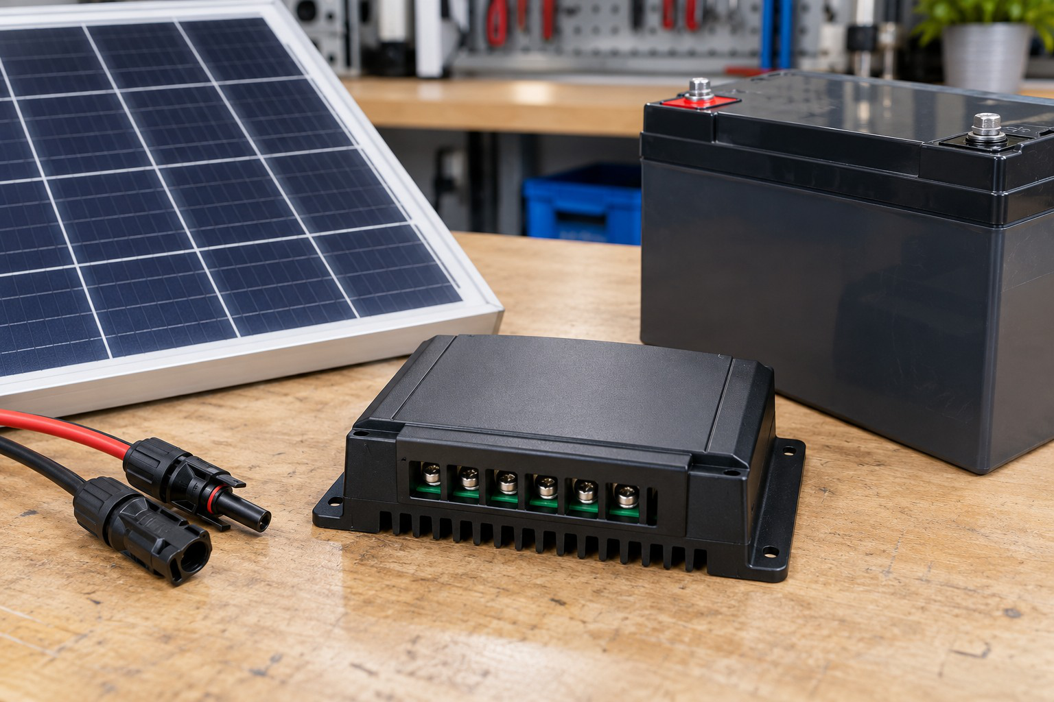
A PV system connects generation, control, storage and load according to its architecture.
Energy estimates need a defined output duration and conversion assumptions. A controller can manage energy flow but does not create energy when irradiance is absent.
Worked Problem 5.66: Maximum Power from a Diode Model
Problem: For
I = 5 − 10⁻⁸[exp(V/0.04) − 1] A
find MPP numerically and calculate fill factor.
Step 1: Find the generating interval.
Voc = 0.801205 V
Search within:
0 < V < 0.801205 V
Step 2: Differentiate power.
dP/dV = I − (VI0/a)exp(V/a)
Set the expression to zero.
Step 3: Numerical solution gives:
Vmp = 0.685297 V
Imp = 4.72425 A
Step 4:
Pmp = 0.685297 × 4.72425 = 3.23751 W
FF = 3.23751/(0.801205 × 5) = 0.808161
Powers at nearby voltages should be smaller.
Worked Problem 5.67: Maximum Power of a Second Model
Problem: For
I = 6 − 2 × 10⁻⁸[exp(V/0.05) − 1] A
find MPP and fill factor.
Step 1:
Voc = 0.975965 V
Search within 0 < V < Voc.
Step 2:
dP/dV = I − (VI0/a)exp(V/a) = 0
Step 3:
Vmp = 0.832432 V
Imp = 5.66003 A
Step 4:
Pmp = 0.832432 × 5.66003 = 4.71159 W
FF = 4.71159/(0.975965 × 6) = 0.804604
The result is a simultaneous interior point, not a multiplication of separate endpoints.
25. Irradiance and Cell-Temperature Effects
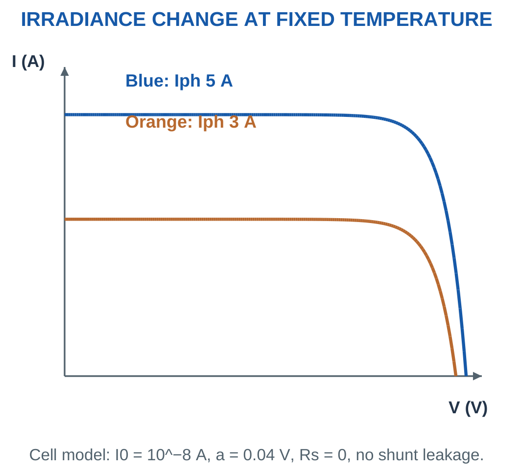
At fixed cell temperature, increasing irradiance raises photocurrent approximately in proportion to irradiance in a simple model.
Short-circuit current therefore changes strongly.
Open-circuit voltage changes more gradually through the logarithmic diode relationship.

Cell Temperature
For a typical silicon module at fixed irradiance, higher cell temperature usually reduces Voc and maximum power. Current changes more modestly.
Use supplied coefficients to quantify the effect. There is no single invented coefficient that applies to every PV technology and condition.
Cell temperature is different from ambient air temperature.
Reference Conditions
Standard test conditions commonly use irradiance 1000 W/m², cell temperature 25°C and a specified reference spectrum.
A nameplate test point does not guarantee constant field output.
Relative Power Coefficient
If αP is a relative power change per degree Celsius:
P(T) = Pref[1 + αP(T − Tref)]
A coefficient in percent per degree must first be divided by 100.
A coefficient in W/°C uses a different numerical formula. Thermal-voltage expressions require absolute temperature in kelvin.
Shading and Mismatch
Unequal illumination and mismatch can alter array curves and introduce multiple peaks.
The matched examples deliberately exclude these effects. Ideal series-parallel scaling should not be applied blindly to shaded unequal strings.
Worked Problem 5.68: Temperature Change to 45°C
Problem: A module gives 300 W at 25°C. Its relative power coefficient is −0.4% per °C. Estimate output at 45°C at fixed irradiance.
Step 1:
αP = −0.004 per °C
ΔT = 45 − 25 = 20°C
Step 2:
Multiplier = 1 − 0.004 × 20 = 0.92
Step 3:
P = 300 × 0.92 = 276 W
Step 4:
Decrease = 24 W = 8%
The result is a local linear approximation rather than a complete recalculation of the diode model.
Worked Problem 5.69: Temperature Change to 50°C
Problem: A module gives 400 W at 25°C with coefficient −0.35% per °C. Estimate output at 50°C.
Step 1:
αP = −0.0035 per °C
ΔT = 25°C
Step 2:
Multiplier = 1 − 0.0035 × 25 = 0.9125
Step 3:
P = 400 × 0.9125 = 365 W
Step 4:
Decrease = 35 W = 8.75%
The negative coefficient gives the expected reduction in the supplied maximum-power model.
Worked Problem 5.70: Temperature Change to 35°C
Problem: A module gives 250 W at 25°C with coefficient −0.45% per °C. Estimate power at 35°C.
Step 1:
αP = −0.0045 per °C
ΔT = 10°C
Step 2:
Multiplier = 1 − 0.0045 × 10 = 0.955
Step 3:
P = 250 × 0.955 = 238.75 W
Step 4:
Decrease = 11.25 W = 4.5%
The coefficient is applied at fixed irradiance. A separate irradiance change would require additional modelling.
Worked Problem 5.71: Irradiance Reduction
Problem: At 1000 W/m², a cell has Iph = 5 A. Find new Isc and Voc at 500 W/m², keeping I0 = 10⁻⁸ A and a = 0.04 V unchanged.
Step 1:
Iph,new = 5 × 500/1000 = 2.5 A
Step 2:
Isc,new = 2.5 A
Step 3:
Voc,old = 0.04 ln(1 + 5/10⁻⁸) = 0.801205 V
Voc,new = 0.04 ln(1 + 2.5/10⁻⁸) = 0.773479 V
Step 4: Interpret the changes.
Current halves, while voltage decreases much less. Voc must not be scaled by the same irradiance ratio.
Worked Problem 5.72: Irradiance Increase
Problem: At 800 W/m², a cell has Iph = 4 A. Find new Isc and Voc at 1000 W/m², with I0 = 10⁻⁸ A and a = 0.04 V unchanged.
Step 1:
Iph,new = 4 × 1000/800 = 5 A
Step 2:
Isc,new = 5 A
Step 3:
Voc,old = 0.04 ln(1 + 4/10⁻⁸) = 0.792279 V
Voc,new = 0.04 ln(1 + 5/10⁻⁸) = 0.801205 V
Step 4: Compare the responses.
Photocurrent increases directly with irradiance in this model, while Voc responds logarithmically.
26. Matched Modules in Series and Parallel
For identical modules at the same irradiance and temperature, series connection adds voltages at the same current.
Parallel connection adds currents at the same voltage.
A series-parallel array can raise both useful voltage and current.


MPP Scaling
For Ns modules per string and Np identical parallel strings:
Vmp,array ≈ NsVmp,module
Imp,array ≈ NpImp,module
Pmp,array ≈ NsNpPmp,module
Ideal endpoint scaling is:
Voc,array = NsVoc,module
Isc,array = NpIsc,module
The endpoint values still describe different operating states.
What Ns Counts
Here Ns counts modules per string.
In a cell-level diode-scale equation, Ns may count series cells. Modules and cells cannot be interchanged within a single equation.
Matching Conditions
The simple relationships assume matched modules under equal conditions. Real shading, mismatch and control can change the result.
The resistance giving an MPP pair is:
Rload = Vmp/Imp
It is an operating-point match rather than a fixed universal internal resistance.
Worked Problem 5.73: Three Modules per String and Two Strings


Problem: Each module has Vmp = 32 V, Imp = 9 A, Voc = 40 V and Isc = 10 A. Use three modules per string and two parallel strings.
Step 1:
Vmp,array = 3 × 32 = 96 V
Step 2:
Imp,array = 2 × 9 = 18 A
Step 3:
Pmp,array = 96 × 18 = 1728 W
Check:
6 × 288 = 1728 W
Step 4:
Voc,array = 3 × 40 = 120 V
Isc,array = 2 × 10 = 20 A
The endpoint values do not replace the simultaneous MPP pair.
PV Modules in an Array


Series and parallel connections change array voltage and current under a matched-module model.
Shading, mismatch and operating controls can alter the result. Module quantities must remain distinct from array quantities.
Worked Problem 5.74: Two Modules per String and Four Strings
Problem: Each module has Vmp = 39 V, Imp = 7.4 A, Voc = 48 V and Isc = 8 A. Use two modules per string and four parallel strings.
Step 1:
Vmp,array = 2 × 39 = 78 V
Step 2:
Imp,array = 4 × 7.4 = 29.6 A
Step 3:
Pmp,array = 78 × 29.6 = 2308.8 W
Check:
Module power = 39 × 7.4 = 288.6 W
Eight-module power = 8 × 288.6 = 2308.8 W
Step 4:
Voc,array = 2 × 48 = 96 V
Isc,array = 4 × 8 = 32 A
There are eight modules in total, but only two modules contribute to each string’s series voltage scaling.
27. PV Power, Efficiency and Energy Numericals
At a specified condition:
P = VI
With incident irradiance G and illuminated area A:
ηPV = VI/(GA)
When maximum power is supplied:
ηPV = Pmp/(GA)
Keep irradiance in W/m² and area in m².


Constant and Varying Power
If constant electrical power P persists for t hours:
E = Pt Wh
E = Pt/1000 kWh
For varying output, add the energy of each interval.
A single midday watt reading does not determine the whole day’s energy without a time profile or equivalent-duration model.
Downstream Losses
If a problem supplies downstream efficiency:
Euseful = ηdownstreamEarray
Do not subtract the same loss twice.
A panel’s electrical watt output has already crossed the optical-conversion boundary. Another unspecified PV efficiency must not be applied again.
Load Energy
A 100 W load operated for two hours uses:
E = 100 × 2 = 200 Wh
Compare energy with energy and instantaneous power capability with simultaneous power requirement.
The examples use supplied durations and efficiencies. They illustrate energy balance rather than weather forecasts or guaranteed production.
Worked Problem 5.75: Energy over Four Equivalent Hours
Problem: An array delivers 800 W for four equivalent hours. Downstream efficiency is 0.9.
Step 1:
Earray = 800 × 4 = 3200 Wh = 3.2 kWh
Step 2:
Euseful = 0.9 × 3.2 = 2.88 kWh
Step 3:
Eloss = 3.2 − 2.88 = 0.32 kWh
Step 4: Keep the boundary clear.
No extra PV conversion factor is applied because the supplied watts are electrical output.
Worked Problem 5.76: Energy over 3.5 Equivalent Hours
Problem: An array delivers 1500 W for 3.5 equivalent hours. Downstream efficiency is 0.85.
Step 1:
Earray = 1500 × 3.5 = 5250 Wh = 5.25 kWh
Step 2:
Euseful = 0.85 × 5.25 = 4.4625 kWh
Step 3:
Eloss = 5.25 − 4.4625 = 0.7875 kWh
Step 4: Interpret the duration.
The equivalent-hour assumption establishes the stated energy. It does not imply that the array produces constant power through every daylight hour.
Worked Problem 5.77: Energy over Five Equivalent Hours
Problem: An array delivers 600 W for five equivalent hours. Downstream efficiency is 0.92.
Step 1:
Earray = 600 × 5 = 3000 Wh = 3 kWh
Step 2:
Euseful = 0.92 × 3 = 2.76 kWh
Step 3:
Eloss = 3 − 2.76 = 0.24 kWh
Step 4: Recover the balance.
2.76 + 0.24 = 3 kWh
The useful energy and loss refer to the same downstream boundary.
28. Electrical Safety in the Laboratory
Electrical laboratory work involves shock, burns, arcs, stored energy, unexpected motion and fire hazards.
Students must use the approved supervised setup, suitable rated instruments and intact leads, following the instructor’s isolation and emergency procedures.


Setup Changes
Before a wiring or range change, stop the experiment and have the supply isolated through the authorised procedure.
A switch label or dark display does not prove that every relevant conductor is de-energised.
Stored energy and multiple supply paths must be considered by the authorised person.
Essential Precautions
- Inspect leads, insulation, connectors and guards before use.
- Keep work areas dry.
- Avoid loose conductive items near exposed circuits.
- Use the correct meter function, rated terminal and range.
- Keep rotating shafts and couplings guarded.
- Secure apparatus as instructed.
- Treat illuminated PV modules as electrical sources.
- Do not bypass interlocks, guards, protective earth or protective devices.
- Report damaged equipment.
- Report abnormal smell, heating or sound promptly.
Emergency Response
Stop work, alert the instructor and use designated emergency isolation only when safe.
Do not touch a person or equipment that may remain energised. Summon assistance and follow trained site procedures.
The diagrams are instructional models. They do not specify a complete safe installation or authorise unsupervised mains work.
Worked Problem 5.78: Meter-Mode Mismatch
Problem: A student has left a lead in the current input and intends to connect the meter across a supply for a voltage reading.
Step 1: Identify that the selected input and function create a different internal path from the intended voltage measurement.
Step 2: Do not energise or trial-connect the current input across the source. Stop and obtain the approved setup.
Step 3: Have the input terminals, function, lead condition and ratings checked under the isolated procedure.
Step 4: Proceed only within the approved supervised experiment. A zero display does not verify a safe connection.
Worked Problem 5.79: Illuminated PV after Disconnection
Problem: A PV module remains illuminated after its load is disconnected. Has open-circuit terminal voltage necessarily disappeared?
Step 1: Load disconnection makes delivered load current approximately zero.
Step 2: The zero-current I–V endpoint is Voc, which can remain nonzero under illumination.
Step 3: Zero delivered terminal power at open circuit does not prove zero source voltage.
Step 4: Follow the approved PV isolation and handling procedure with supervision.
Disconnecting a load changes the operating point; it does not automatically extinguish the source.
Worked Problem 5.80: Missing Coupling Guard
Problem: The electrical supply to a motor experiment is being changed while a coupling guard is absent.
Step 1: Treat exposed rotating parts and unexpected startup as a separate hazard from the circuit calculation.
Step 2: Stop the experiment and alert the instructor rather than continuing because the motor is presently stationary.
Step 3: Restore approved guarding and the controlled isolated setup before an authorised restart.
Step 4: Do not bypass an interlock or hold a moving coupling by hand to finish a measurement.
29. Protective Earth, Residual Current and Stored Energy
Protective earth connects designated exposed conductive parts to the protective system required by the equipment design.
Neutral is an intended circuit conductor with a different function. The two must not be treated as interchangeable return wires.

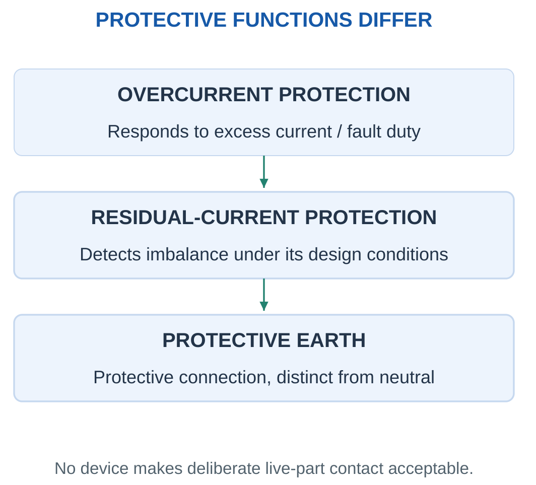
Overcurrent Protection
A fuse or circuit breaker responds to overcurrent according to its rating and operating characteristic.
It does not perform every other protective function.
Residual-Current Protection
A residual-current device compares outgoing and returning current and responds to imbalance under its design conditions.
Neither residual-current nor overcurrent protection makes deliberate live-part contact acceptable.
Protective measures work together within the approved system.
Capacitor Energy
Stored capacitor energy is:
W = CV²/2
Removing an external supply does not automatically establish zero capacitor voltage.
Energy removal and verification require the approved procedure, suitable equipment and supervision. Improvised short circuits are not a substitute.
Meter Input Paths
A meter in current mode can have a very different input path from voltage mode.
Connecting that current input across a voltage source can create a fault. Stop and obtain the correct connection before energising.
Contact Risk and Numerical Models
Risk depends on contact conditions, current path, duration, available energy and protection.
The examples calculate circuit quantities and stored energy. They do not define a universal safe-touch voltage or current.
Illuminated PV, capacitors, rotating machines and separate AC/DC sources require their own energy-path awareness.
Capacitor and Stored Energy

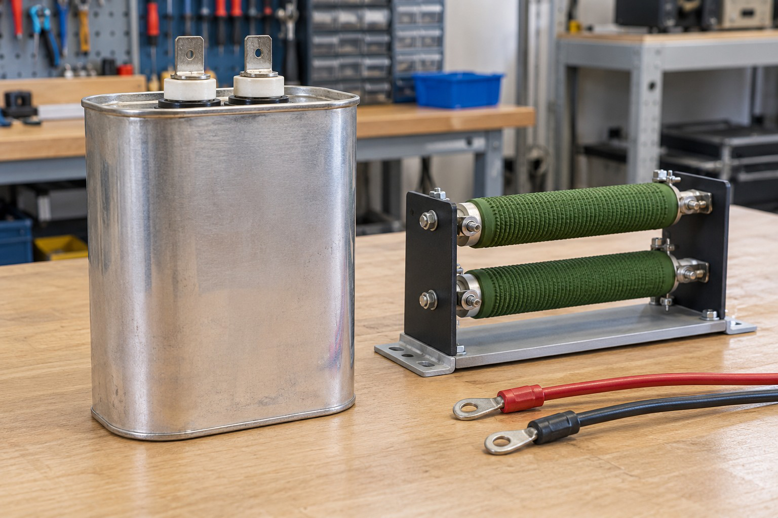
A capacitor can retain energy after external isolation.
The one-half CV-squared relation uses the stated capacitance and voltage. Source isolation and a verified zero-energy state are different conditions.
Worked Problem 5.81: Energy in a 470 μF Capacitor
Problem: A 470 μF capacitor has 100 V across it. Find stored energy and energy remaining at half voltage. Explain what external isolation alone establishes.
Step 1:
C = 470 × 10⁻⁶ = 0.00047 F
W = 0.5 × 0.00047 × 100² = 2.35 J
Step 2:
Wremaining = C(V/2)²/2 = W/4
Wremaining = 0.5875 J
Step 3: External isolation stops that specified source path but does not prove zero capacitor voltage or energy.
Step 4: Follow authorised stored-energy control and verification procedures. Do not infer safety from switch position or improvise a short circuit.
Worked Problem 5.82: Energy in a 220 μF Capacitor
Problem: A 220 μF capacitor has 300 V across it. Find stored energy and energy at half voltage.
Step 1:
C = 0.00022 F
W = 0.5 × 0.00022 × 300² = 9.9 J
Step 2:
Wremaining = 9.9/4 = 2.475 J
Step 3: External isolation does not itself establish zero voltage or energy.
Step 4: Use authorised verification with suitable equipment and supervision.
The smaller capacitance stores more energy than in the previous example because voltage enters as its square.
30. Formula Sheet and Examination Checks
Mechanical and DC Motor Relationships
| Quantity | Formula and Condition |
|---|---|
| Shaft angular speed | ω = 2πN/60 |
| Mechanical power | P = Tω |
| Torque from kilowatts and rpm | T ≈ 9550P(kW)/N |
| Steady DC armature | Eb = V − IaRa, neglecting brush drop |
| DC generated/back EMF | Eb = PΦZN/(60A) |
| DC developed power | Pdev = EbIa |
| DC developed torque | Tdev = KΦIa |
| Torque from developed power | Tdev = Pdev/ω for nonzero speed |
| Shaft output | Pshaft = Pdev − Prot |
| Speed ratio | N2/N1 = (Eb2/Eb1)(Φ1/Φ2) |
| Shunt field current | If = V/Rf |
| Shunt line current | IL = Ia + If |
| Armature copper loss | Ia²Ra |
| Whole-motor efficiency | η = Pshaft/Pin |
BLDC and Induction Relationships
| Quantity | Formula and Condition |
|---|---|
| Pole pairs | p = P/2 |
| BLDC electrical frequency | fe = pN/60 |
| Ideal six-step interval rate | 6fe |
| Intervals per mechanical revolution | 6p |
| Synchronous field speed | Ns = 120f/P rpm |
| Slip fraction | s = (Ns − N)/Ns |
| Rotor speed | N = Ns(1 − s) |
| Rotor frequency | fr = sf |
| Running rotor EMF | E2s = sE20 |
| Running rotor reactance | X2s = sX20 |
| Rotor copper loss | sPgap |
| Developed mechanical power | (1 − s)Pgap |
| Developed torque | Pgap/ωs = Pdev/ωr |
| Balanced motor input | Pin = √3VLIL PF |
PV and Energy Relationships
| Quantity | Formula and Condition |
|---|---|
| Incident optical power | GA |
| Electrical output | VI |
| Maximum output | VmpImp |
| Fill factor | Pmp/(VocIsc) |
| PV efficiency | Pmp/(GA) |
| Simplified current | Iph − I0[exp(V/a) − 1] |
| Simplified short-circuit current | Isc = Iph |
| Simplified open-circuit voltage | Voc = a ln(1 + Iph/I0) |
| MPP resistive load | Vmp/Imp |
| Relative temperature model | Pref[1 + αP(T − Tref)] |
| Matched array voltage | NsVmp,module |
| Matched array current | NpImp,module |
| Constant-power energy | Pt |
| Capacitor stored energy | CV²/2 |
Fast Checks
- Back EMF is below supply voltage in the stated positive-current motoring model.
- Back-EMF power is a conversion term, while resistance power is heating.
- Developed and shaft torques differ when rotational losses are supplied.
- Shunt line current includes field and armature currents.
- A 4% slip is inserted as 0.04.
- Loaded induction rotor speed is below synchronous speed in normal motoring.
- Rotor current frequency differs from shaft revolutions per second.
- Voc and Isc give zero terminal power at their separate endpoints.
- Fill factor and conversion efficiency have different denominators.
- Electrical watts do not establish daily energy without time.
- Source isolation does not prove all stored energy has disappeared.
Complete DC Armature Revision Check
For V = 100 V, Ra = 1 Ω and Ia = 10 A:
Eb = 100 − 10 × 1 = 90 V
Armature input:
VIa = 1000 W
Copper loss:
Ia²Ra = 100 W
Developed power:
EbIa = 900 W
At 1000 rpm:
ω = 104.72 rad/s
Tdev = 900/104.72 = 8.594 N·m
If rotational loss is 100 W:
Pshaft = 800 W
Tshaft = 800/104.72 = 7.639 N·m
Whole-motor efficiency also requires any field input to be included.
Induction and PV Revision Check
A four-pole 50 Hz induction motor at 4% slip has:
Ns = 1500 rpm
N = 1440 rpm
fr = 2 Hz
These are three different speed/frequency measures.
For a separate PV module with MPP 30 V and 8 A:
Pmp = 240 W
If Voc = 40 V and Isc = 9 A:
FF = 240/(40 × 9) = 0.6667
The endpoint rectangle is 360 W, rather than delivered output. Combining quantities from different definitions can produce a plausible-looking but physically incorrect result.
31. Short Questions with Answers
1. Why Is DC Motor EMF Called Back EMF?
Its referenced effect opposes the applied armature supply.
It reduces the voltage available across armature resistance while representing energy conversion rather than a heat loss by itself.
In the steady balance, V = Eb + IaRa. The product EbIa is developed conversion power.
2. Can a Motor Produce Torque at Zero Speed?
Yes. Electromagnetic torque can be finite at standstill.
Mechanical power Tω is zero because speed is zero. The direct relation Tdev = KΦIa explains finite starting torque.
Zero shaft power does not automatically mean zero torque.
3. Why Does a DC Motor Need Starting-Current Control?
At standstill, back EMF is approximately zero.
The supply is then applied across a low armature resistance in the simple resistance-only model. The uncontrolled estimate V/Ra can be excessive.
A starter or suitable electronic controller limits current according to the intended machine operation.
4. Why Is Shunt Line Current Different from Armature Current?
Part of the line current flows through the parallel field branch.
IL = Ia + If
Whole-motor input includes both branch powers. Armature current must be obtained after subtracting field current from line current.
5. Does Field Weakening Always Preserve Torque?
No. Torque per armature ampere decreases with flux.
The speed relation can predict an increase in speed, but torque capability remains constrained by the flux-current relationship and machine limits.
Higher speed and unchanged current do not imply unchanged torque.
6. How Does BLDC Commutation Differ from Brushed DC Commutation?
A BLDC drive electronically switches stator currents in relation to rotor position.
A brushed DC machine uses sliding brushes and a mechanical commutator for its armature-switching function.
Brushless construction transfers switching into the electronic system rather than eliminating commutation.
7. Why Are Pole Pairs Needed in BLDC Frequency Calculations?
A mechanical revolution contains one electrical cycle per pole pair.
Therefore:
fe = (P/2)N/60
Using N/60 alone would describe electrical frequency only for the corresponding one-pole-pair case.
8. Why Must an Induction Rotor Normally Lag Its Field?
Relative motion induces rotor EMF and current.
At exact synchronous speed, the elementary steady induction mechanism has no relative field variation to sustain nonzero load torque.
Positive slip is therefore required for ordinary loaded motoring.
9. What Does a Slip of 3% Mean?
The rotor runs at 97% of synchronous speed in the normal motoring case.
s = 0.03
N = 0.97Ns
Rotor current frequency is 0.03 times supply frequency. The percentage is not a universal rpm difference.
10. What Is Air-Gap Power Divided Into?
The simple rotor model divides it into:
sPgap as rotor copper loss.
(1 − s)Pgap as developed mechanical power.
Further rotational losses reduce useful shaft output.
11. Does a PV Module Deliver VocIsc Watts?
No. Voc occurs at zero current, while Isc occurs at zero voltage.
Maximum useful power comes from the simultaneous pair Vmp and Imp.
The product VocIsc forms the denominator in fill factor rather than an output operating point.
12. How Do Fill Factor and Efficiency Differ?
Fill factor compares Pmp with VocIsc.
PV conversion efficiency compares electrical power with incident optical power GA.
The denominators have different physical meanings. A fill-factor value alone does not establish conversion efficiency.
13. Is a Battery Necessary in Every PV System?
No. Storage depends on architecture and operating needs.
A PV array, converter and load or grid can operate in an architecture without a battery.
Storage is included when required by the intended energy-use pattern.
14. Does Turning Off the Supply Remove Every Hazard?
No. Stored capacitor energy, separate sources, illuminated PV and mechanical motion may remain.
The approved isolation and verification procedure is required.
A switch position or dark display is not proof of a zero-energy condition.
15. Are Residual-Current and Overcurrent Protection Identical?
No. They respond to different measured fault conditions.
Correct protection and protective earth work together. Neither function makes deliberate contact with exposed live parts acceptable.
They should not be treated as interchangeable protective measures.
32. Complete Examination Answers
1. Explain the DC Motor Principle and Back EMF
A current-carrying conductor in a magnetic field experiences force:
F = BIl sin θ
In a DC motor, forces on opposite armature sides form a torque-producing couple. The armature current pattern must change as the rotor turns so that useful torque continues in the intended direction.
A brushed machine uses a commutator and brushes for this switching function.
Rotation also generates an EMF because armature conductors cut magnetic flux. Under the normal motoring reference, the generated voltage opposes the applied supply and is called back EMF.
The simple steady armature equation is:
V = Eb + IaRa
Thus:
Ia = (V − Eb)/Ra
At starting, back EMF is approximately zero. A low resistance then gives a large uncontrolled-current estimate, explaining the need for current limiting.
When load increases within the operating range, a small speed reduction lowers back EMF. The larger resistance voltage raises current and torque.
Multiplying the voltage equation by current gives:
VIa = EbIa + Ia²Ra
Back-EMF power is developed conversion power. The resistance term is copper heat. The distinction connects the electrical equation to the machine’s energy balance.
2. Explain Developed Torque, Power and Speed Control
Developed mechanical power is:
Pdev = EbIa
For nonzero speed:
Tdev = EbIa/ω
Substitution of the DC EMF equation gives:
Tdev = [PZ/(2πA)]ΦIa
For a fixed machine, torque is proportional to flux times armature current.
At constant flux, torque follows current linearly. In an unsaturated series comparison, flux also follows current, giving an approximate square law.
The speed relationship is:
N ∝ (V − IaRa)/Φ
Armature-voltage control changes the available back EMF. Resistance control adds voltage drop and heat loss. Field control changes the flux denominator.
Field weakening can raise speed but lowers torque per ampere and remains subject to current and mechanical limits.
Shaft output is obtained after subtracting specified rotational losses:
Pshaft = Pdev − Prot
At standstill, use the direct torque relation instead of dividing zero developed power by zero speed.
3. Compare DC Motor Field Connections
A separately excited motor has an independent field supply.
A shunt motor connects the field in parallel with the armature. Its line current is the sum of field and armature currents.
A series motor carries armature current through its field, so field and armature currents are equal in the simple connection.
A compound motor combines shunt and series field effects. Cumulative compounding makes their principal field contributions aid.
A PMDC motor uses permanent magnets for the main field.
Under constant flux, developed torque is proportional to armature current. Under the unsaturated series approximation, flux is proportional to current and torque is approximately proportional to current squared.
Classical shunt applications emphasise approximately steady speed. Classical series applications emphasise high starting torque.
A series motor requires suitable loading and control to prevent no-load overspeed.
Actual application choice also depends on ratings, duty, environment, maintenance and the associated drive.
4. Explain BLDC Construction and Electronic Commutation
A BLDC motor uses a permanent-magnet rotor and stationary phase windings supplied through an inverter.
The DC source feeds the drive, while phase voltages and currents are switched according to rotor position and control strategy.
Position information can come from sensors or a suitable estimator.
A basic six-step method advances through six phase-current states per electrical cycle. Each state includes a positive phase, a negative phase and a floating phase.
Actual mapping depends on winding, sensor and direction conventions.
With P poles:
fe = (P/2)N/60
A mechanical revolution contains one electrical cycle per pole pair.
Back-EMF-based sensorless estimation has limited information at standstill, requiring a suitable startup method.
Brush wear is avoided, but coordinated electronics and current control remain necessary. Fans, pumps and compact drives are illustrative contexts.
Efficiency must be calculated from supplied input and output boundaries rather than inferred from brushless construction alone.
5. Explain Rotating Field, Synchronous Speed and Slip
Balanced three-phase currents in windings displaced by 120 electrical degrees produce an ideal constant-amplitude rotating resultant field.
The field speed is:
Ns = 120f/P rpm
Increasing pole count reduces mechanical field speed at a fixed frequency.
A cage rotor has induced current because of relative motion between rotor conductors and the rotating field.
Slip is:
s = (Ns − N)/Ns
Rotor speed is:
N = Ns(1 − s)
Rotor current frequency is:
fr = sf
At standstill, slip is one. At synchronous speed, slip is zero.
A loaded rotor requires positive slip in the elementary motoring model because relative motion is needed to induce rotor current and torque.
At low slip, torque initially rises approximately with slip. The complete characteristic has a maximum, so the low-slip trend cannot support unlimited load.
6. Explain Induction-Motor Power Flow and Torque
Stator input supplies stator losses and air-gap power.
Within the simple rotor model:
Pcu,rotor = sPgap
Pdev = (1 − s)Pgap
Subtract specified rotational losses to obtain shaft output:
Pshaft = Pdev − Prot
At nonzero speed:
Tdev = Pdev/ωr
Since rotor and synchronous angular speeds are related by:
ωr = (1 − s)ωs
the same developed torque is:
Tdev = Pgap/ωs
At standstill, mechanical developed power is zero even if torque is finite. The synchronous-speed expression helps interpret this limit.
Shaft torque differs from developed torque when rotational loss is present.
For a supplied shaft output, efficiency gives electrical input. Power factor then connects input watts with balanced three-phase apparent power and line current.
Each step must use the correct power boundary.
7. Explain the Single-Diode PV Model and Curves
The model combines photocurrent Iph, a parallel diode, shunt resistance Rsh and series resistance Rs.
With delivered output current positive:
Vd = V + IRs
The terminal current is:
I = Iph − I0[exp((V + IRs)/a) − 1] − (V + IRs)/Rsh
The scale a includes ideality, absolute temperature and the appropriate series-cell count.
For the simplified zero-series-resistance, negligible-leakage model:
I = Iph − I0[exp(V/a) − 1]
The endpoints are Isc at zero voltage and Voc at zero current. Both have zero terminal power.
The P–V curve is formed from P = VI and reaches a maximum at Vmp and Imp.
Pmp = VmpImp
Fill factor is Pmp divided by VocIsc. Conversion efficiency is electrical output divided by incident optical power GA.
Irradiance and temperature change the curve and maximum-power point. Cell-level and module-level parameters must remain consistent.
8. Explain Essential Electrical Laboratory Precautions
Use the authorised supervised setup with intact rated instruments, leads, guards and approved protective arrangements.
Inspect apparatus before energising. Identify sources, meter functions, terminals and ranges.
Wiring and range changes require the approved isolation process.
A switch position or dark display does not verify the absence of every source or stored energy. Capacitors can retain CV²/2, and illuminated PV can retain open-circuit voltage.
Protective earth, neutral, overcurrent protection and residual-current protection have distinct functions. They must not be bypassed or interchanged.
Keep rotating shafts and couplings guarded. A stationary machine can still present unexpected-startup risk.
Keep the area dry and report damaged equipment or abnormal operation.
In an emergency, stop work, alert the instructor, use designated isolation only when safe and summon assistance.
Do not touch a potentially energised casualty or improvise a live-circuit rescue.
33. Integrated Revision of Energy Boundaries
Armature Input and Whole-Motor Input
An armature equation describes the armature branch. It does not automatically include a separately supplied field or a parallel shunt field.
For an armature-only boundary:
Parmature = VIa
For a shunt motor supplied from one source:
Pin = VIL
Because IL includes field current, the two powers differ.
The distinction is especially important in efficiency problems. A correct shaft output divided by the wrong input still gives an incorrect efficiency.
A useful solution names the input boundary before calculating branch currents. It then checks that total input equals useful output plus the losses inside that boundary.
Developed Mechanical Power and Shaft Output
Developed power represents internal electromagnetic conversion.
Shaft output is the useful mechanical power remaining after rotational and other specified downstream losses.
For DC machines:
Pdev = EbIa
For the elementary induction rotor model:
Pdev = (1 − s)Pgap
In both cases:
Pshaft = Pdev − Prot
The common structure makes it easier to remember why developed and shaft torques differ.
Stator Input and Air-Gap Power
The induction-motor rotor power split begins with air-gap power.
Stator copper and core losses lie upstream of that rotor boundary. Therefore, sPgap is rotor copper loss, while sPin is generally not the same quantity.
If a question starts from total electrical input, the relevant upstream losses must be identified before using a rotor power relation.
This is an example of why a familiar formula should not be applied to a similarly named but physically different power.
Optical Input and Electrical PV Output
For a PV module, GA is incident optical power.
The electrical output VI is measured at one operating point. Their ratio gives conversion efficiency under the stated conditions.
If electrical output is already supplied, it has already crossed the optical-conversion boundary. Applying another unspecified PV efficiency would reduce the result twice.
Later controller or storage efficiencies belong to their own downstream stages.
34. Integrated Revision of Speed and Frequency
RPM and Radians per Second
RPM counts complete revolutions per minute.
Radians per second measures angular displacement per second. The conversion is:
ω = 2πN/60
The factor 2π converts revolutions into radians, and division by 60 converts minutes into seconds.
Torque calculations using P = Tω require this angular-speed unit.
The 9550 shortcut combines the same conversion with kilowatts. It does not remove the need to recognise which units are being used.
Mechanical Revolutions and Electrical Cycles
A multi-pole machine can complete several electrical cycles in one mechanical revolution.
With p pole pairs:
fe = pN/60
The mechanical rate N/60 is multiplied by pole pairs to obtain electrical frequency.
For a rotating induction field, the same relationship rearranges into:
Ns = 60f/p
The field speed is fixed by frequency and pole count under the elementary model.
Rotor Frequency and Shaft Frequency
An induction rotor has a mechanical revolution rate and an induced-current frequency.
These are generally different.
For a four-pole 50 Hz motor at 1440 rpm:
- Mechanical rotation rate is 24 revolutions/s.
- Synchronous speed is 1500 rpm.
- Slip is 4%.
- Rotor current frequency is 2 Hz.
Substituting one of these quantities in place of another changes the physical meaning of the equation.
Slip Fraction and Relative RPM
Relative speed is:
Ns − N
Slip fraction divides this difference by Ns.
Thus:
Ns − N = sNs
A fixed percentage does not correspond to one universal rpm difference. Four percent of 1500 rpm is 60 rpm, while four percent of 750 rpm is 30 rpm.
The percentage is meaningful only relative to its synchronous-speed base.
35. Integrated Revision of PV Operating Points
Simultaneous Voltage and Current
Electrical power is a voltage-current product at one operating point.
At short circuit, voltage is zero. At open circuit, current is zero.
The maximum-power point lies between those endpoints and uses the simultaneous pair Vmp and Imp.
Combining Voc with Isc creates a useful reference rectangle, but not delivered output.
This principle also applies to measured data: values taken under different irradiance or temperature conditions should not be multiplied as though they described one state.
Fill Factor and Conversion Efficiency
Fill factor describes how effectively the I–V curve occupies its endpoint rectangle.
Conversion efficiency describes how much incident optical power becomes useful electrical power.
A module’s fill factor can be calculated from Voc, Isc, Vmp and Imp. Its conversion efficiency additionally requires irradiance and illuminated area.
The two ratios can both be dimensionless while still representing different physical ideas.
A Matching Resistance Is Condition-Specific
At one MPP:
Rload = Vmp/Imp
A resistor of that value intersects the supplied curve at the stated point.
If conditions change, the curve and MPP can move. A fixed resistor then need not remain at maximum power.
Maximum-power tracking addresses this changing electrical operating condition. It is distinct from physically changing the panel’s orientation.
Cell, Module and Array Levels
A cell-level diode model uses cell-level voltage and parameters.
A module combines cells. An array combines modules and strings.
Series counts in these models do not necessarily count the same object. A series-cell count in an exponential voltage scale cannot be replaced by a module count without redefining the model.
Clear labels prevent a numerically plausible but physically inconsistent substitution.
36. Common Examination Mistakes
Dividing Power by RPM Directly
The equation is P = Tω, with ω in rad/s.
Use 2πN/60 or the stated kilowatt-rpm shortcut. Direct division by rpm omits the conversion.
Calling Back EMF a Copper Loss
Back EMF times armature current is developed conversion power.
Copper heating is current squared times resistance. These terms arise from the same voltage balance but represent different outcomes.
Using Line Current in Every DC Formula
A shunt motor’s line current includes field current.
Armature back EMF and copper loss require Ia, obtained after accounting for the field branch.
Applying the Series Torque Square Law Universally
The square law depends on an unsaturated field with flux proportional to current.
Constant-flux torque is proportional to current. Saturation changes the series approximation.
Using Voltage Ratio Alone for Speed
The relevant ratio contains back EMF and flux.
Calculate V − IaRa at both operating points whenever those terms are represented in the model.
Treating Electrical Hertz as Mechanical Revolutions per Second
Include pole pairs.
For induction motors, additionally distinguish rotating-field speed, actual rotor speed and rotor electrical frequency.
Inserting Slip Percent as a Whole Number
Convert 3% into 0.03 before using N = Ns(1 − s), fr = sf or rotor power equations.
Using Stator Input in a Rotor Power Split
The relation sPgap uses air-gap power.
Stator input requires upstream loss accounting before the rotor boundary is reached.
Multiplying Voc and Isc as Delivered Power
They occur at different points.
Use VmpImp for maximum output or VI at another simultaneous operating point.
Calling Fill Factor Efficiency
The denominator of fill factor is VocIsc.
The denominator of PV conversion efficiency is GA.
Applying Conversion Loss Twice
Electrical PV output already accounts for optical conversion.
Apply only explicitly stated downstream efficiencies after that boundary.
Treating Isolation as Verification
A disconnected source does not automatically establish zero capacitor energy, zero illuminated PV voltage or zero mechanical motion.
The approved verification procedure remains necessary.
37. Final Formula-Based Practice Connections
Connecting Voltage, Power and Torque in a DC Motor
Begin with terminal voltage and armature current.
Use resistance to find back EMF. Multiply back EMF by current to find developed mechanical power.
Convert speed into rad/s and divide developed power by angular speed to find developed torque.
If rotational loss is supplied, subtract it before calculating shaft torque.
If total efficiency is requested, include field input within the selected whole-motor boundary.
This order prevents the voltage equation, power balance and mechanical equation from being used as unrelated fragments.
Connecting Frequency, Slip and Power in an Induction Motor
Use supply frequency and pole count to find synchronous speed.
Use slip to find rotor speed and rotor current frequency.
Use air-gap power and slip to divide rotor input into copper loss and developed mechanical power.
Subtract rotational loss for shaft output.
Use synchronous speed with air-gap power or rotor speed with developed power to calculate the same developed torque.
A final comparison of these two torque expressions checks the consistency of the solution.
Connecting a PV Curve with Energy
Use the curve or supplied operating values to identify electrical power.
If maximum power is requested, use the simultaneous MPP pair.
If efficiency is requested, compare output with irradiance times area.
If energy is requested, include duration or integrate the output profile.
If useful load energy is requested, apply only the stated downstream conversion efficiency.
Each stage introduces a new boundary or time basis. Keeping that progression explicit reduces double counting.
Connecting Numerical Work with Laboratory Practice
A classroom circuit model identifies current, voltage, power or stored energy under assumptions.
A physical experiment additionally requires suitable ratings, guarding, connection checks, isolation and verification.
The equations support understanding, but they do not replace the authorised procedure.
A final answer should therefore state the model and requested quantity clearly while avoiding unsupported claims about unrestricted operation or a universally safe condition.