
University: Dr. A.P.J. Abdul Kalam Technical University (AKTU)
Programme: B.Tech First Year, Semester I & II
Course Codes: AME101A / AME201A
Branches: Common to All
Unit: I — Engineering Mechanics and Strength of Materials (Basics)
Introduction
Engineering Mechanics and Strength of Materials explains how loads travel through a component, how supports balance forces and how materials resist deformation. The same principles apply to a server shelf, laptop frame, antenna support, robot arm and vehicle chassis.
Engineering mechanics establishes the external forces and moments acting on a selected body. Strength-of-materials concepts then connect internal loading with stress, strain, stiffness and material response.
A useful solution begins with a clear model. The selected body, load directions, support conditions and dimensions must be identified before equations are written. A correct numerical substitution cannot repair an incorrect free-body diagram.
Topic Map
| Topic | Main Coverage |
|---|---|
| Force systems | Force types, components and resultants |
| Free-body diagrams | Selected bodies, support reactions and load paths |
| Equilibrium | Force balance, moments, couples and load sharing |
| Stress and strain | Average normal stress, shear stress and dimensional change |
| Elasticity | Hooke’s law, Young’s modulus and axial stiffness |
| Beam loading | Point loads, UDLs, combined loading and cantilevers |
| Material properties | Stiffness, strength, hardness, toughness and ductility |
| Material families | Metals, polymers, ceramics and composites |
| Applications | Laptop frames, server racks, antenna supports, robot arms and EV chassis |
| Revision | Formulae, worked problems, short answers and examination answers |
Quick Vocabulary
| Symbol | Meaning |
|---|---|
| F | Force |
| W | Weight or a specified resultant load |
| M | Moment |
| σ | Normal stress |
| τ | Shear stress |
| ε | Engineering strain |
| E | Young’s modulus |
| A | Resisting cross-sectional area |
| L or L0 | Original length or stated span |
| ΔL | Change in length |
| w | Uniform load per unit length |
| ρ | Density |
| RA, RB | Support reactions |
How to Study This Unit
- Select the body before drawing forces.
- Mark supports, load directions and dimensions.
- Balance moments as well as forces.
- Distinguish mass in kilograms from force in newtons.
- Use one consistent length unit within an equation.
- Identify the resisting area and loading direction.
- Apply Hooke’s law only within the stated linear range.
- State beam and load idealisations.
- Separate stiffness requirements from strength requirements.
- Screen material candidates against constraints before comparing mass or cost.
Model Conventions
Loads are static unless stated otherwise. Supports and equal sharing are idealisations. Material properties and allowable limits in numerical problems are supplied example data.
Average direct stress does not describe local bending, stress concentrations or buckling. An illustration supplies context, while numerical dimensions and constraints come from the stated problem.
A useful answer explains the model, writes the equation, substitutes with units and checks whether the result matches the expected direction and trend.
1. Engineering Mechanics and a Component’s Job
Engineering mechanics describes how forces affect bodies. A force can change motion, cause rotation, deform a component or produce several effects together.
Strength-of-materials ideas describe how internal force intensity and deformation relate to material properties and component geometry.

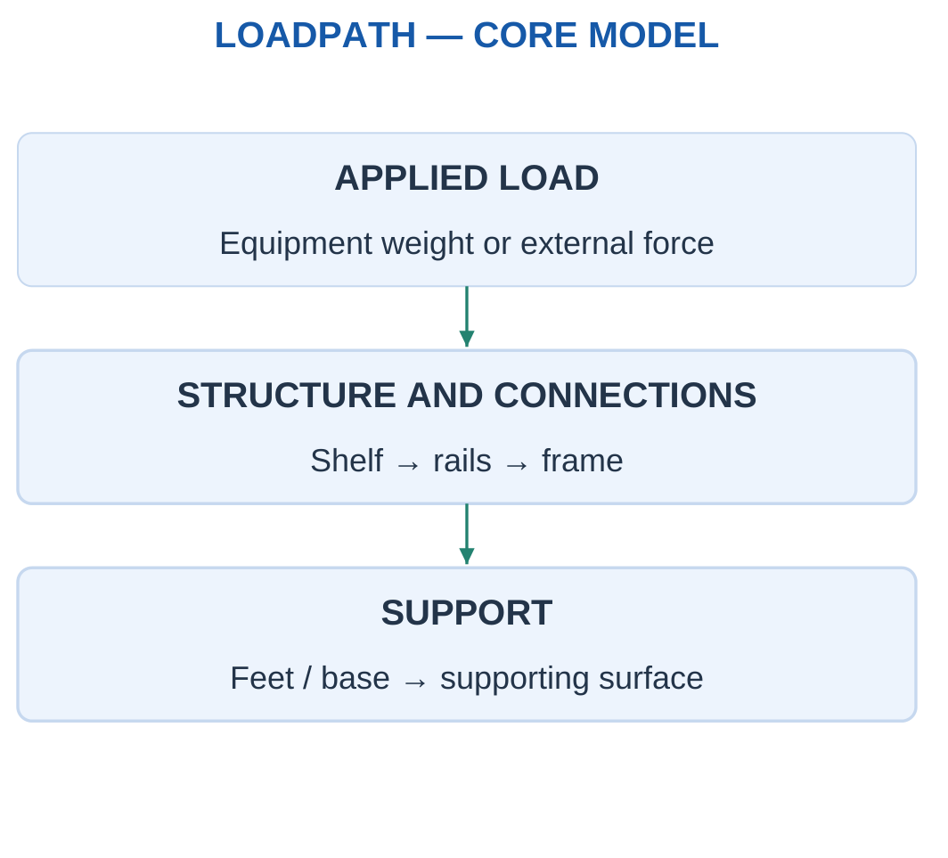
A useful first-year solution starts with the component’s function.
A server shelf supports equipment. A laptop frame protects and locates parts. An antenna support carries weight and lateral loading. A robot arm positions a payload.
The same force-balance equation can appear in several products, but the selected body and support model can differ.
Four Questions Before Calculating
- What body or component is being studied?
- Which external forces and moments act on it?
- How do supports and connections transfer the load?
- Is the question about equilibrium, stress, deformation or material choice?
Scope of the Basic Models
The introductory models use forces, moments, average direct stress, strain and simple beam loading.
An average-stress calculation does not establish local stress around a hole, complete fatigue life or buckling resistance without additional analysis.
A correct result therefore includes its assumptions. The calculated quantity should not be presented as a complete product rating.
Worked Problem 1.1: Mass Becomes a Gravitational Load
Problem: A supported assembly has mass 12 kg. Use g = 9.81 m/s². Find its weight and total upward reaction when it is at rest with no other vertical load.
Step 1: Convert mass into weight.
W = mg = 12 × 9.81 = 117.72 N
Mass and force have different units.
Step 2: Choose upward as positive.
ΣFy = 0
R − W = 0
Step 3: Calculate the total support resultant.
R = 117.72 N upward
This is the sum of all supporting reactions, rather than necessarily one foot or rail force.
Step 4: If several supports share equally, divide R by the stated support count. Equal sharing requires symmetry or an explicit assumption.
Do not multiply by g again when a later problem gives a load directly in newtons.
Worked Problem 1.2: Weight of a Larger Assembly
Problem: A supported assembly has mass 25 kg. Find its weight and total upward reaction using g = 9.81 m/s².
Step 1:
W = 25 × 9.81 = 245.25 N
Step 2: For vertical equilibrium:
R − 245.25 = 0
Step 3:
R = 245.25 N upward
The downward weight and upward support resultant balance.
Step 4: Individual support forces require a load-sharing model. Two supports do not automatically carry equal loads if geometry or loading is asymmetric.
The result establishes equilibrium under the given loading. It does not establish support capacity.
2. Types of Forces and Their Effects
A force is a vector. Its magnitude, direction and line of action all matter.
Contact forces arise through physical interaction, such as support reaction or cable tension. Body forces, such as gravity, act throughout the mass and can be represented by an appropriate resultant.

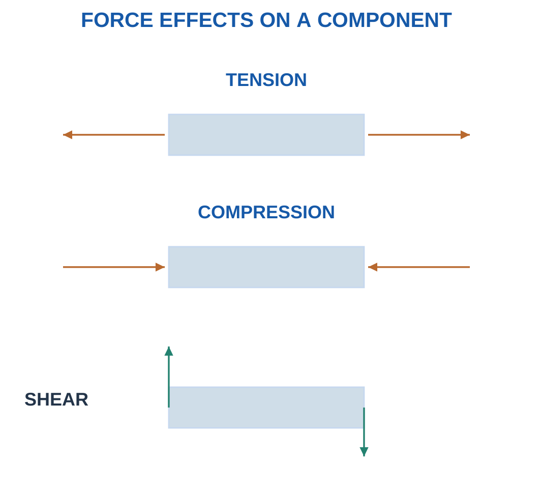
Axial tension tends to lengthen a component. Axial compression tends to shorten it.
A transverse load can bend a beam. Opposite tangential actions can shear material. A twisting moment produces torsion.
One component can experience several loading effects simultaneously.
Common Loading Actions
| Action | Introductory Effect | Example |
|---|---|---|
| Tension | Pulling along a member | Tie or support cable |
| Compression | Pushing along a member | Short support post |
| Transverse loading | Bending tendency | Equipment shelf |
| Shear | Relative sliding tendency | Idealised pin plane |
| Couple or torque | Rotational tendency | Bracket or shaft |
Direction and Line of Action
A 100 N force to the right differs from a 100 N force upward.
Even equal parallel forces can produce different moments if their lines of action differ.
External loads act on the selected body. Internal forces act across imaginary cuts inside that body. They should not be placed on a whole-body diagram as separate additional external loads.
Worked Problem 1.3: Collinear Forces in the Same Direction
Problem: Two horizontal forces act on one body. A 120 N force and an 80 N force both point right. Find their resultant and a balancing force.
Step 1: Choose right as positive.
F1 = +120 N
F2 = +80 N
Step 2: Add algebraically.
Rx = 120 + 80 = 200 N
Step 3: The balancing force is opposite.
Fbalance = −200 N
It points left.
Step 4: Zero resultant force does not by itself prove rotational equilibrium. The application position of the balancing force must also be considered.
Worked Problem 1.4: Opposing Collinear Forces
Problem: A 200 N force points right and a 75 N force points left.
Step 1:
F1 = +200 N
F2 = −75 N
Step 2:
Rx = 200 − 75 = 125 N
The resultant points right.
Step 3:
Fbalance = −125 N
The balancing force points left.
Step 4: Force balance and moment balance remain separate requirements. Equal opposite forces with separated lines of action can form a couple.
3. Units, Mass, Weight and Force Components
Mass is measured in kilograms. Force is measured in newtons.
Near Earth’s surface:
W = mg
Use the gravitational acceleration supplied by the problem. These examples use 9.81 m/s² when required.
A mass of 10 kg has weight 98.1 N under this assumption.

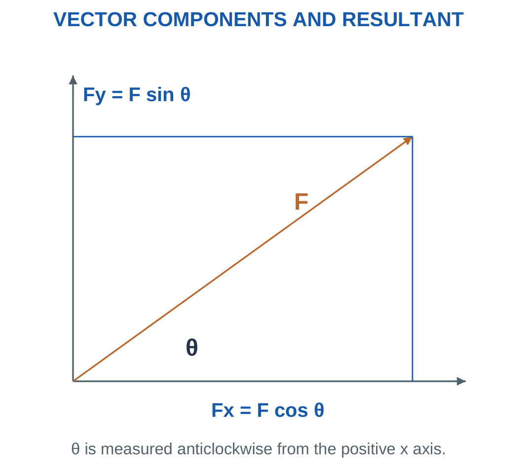
For force F at angle θ from positive horizontal:
Fx = F cos θ
Fy = F sin θ
Assign signs from the chosen axes.
If the angle is measured from vertical, the appropriate sine and cosine roles change.
Useful Conversions
- 1 kN = 1000 N.
- 1 m = 1000 mm.
- 1 cm² = 100 mm².
- 1 N/mm² = 1 MPa.
- 1 N·m = 1000 N·mm.
- 1 GPa = 1000 MPa.
A load already supplied in N or kN is already a force. Apply mg only when converting mass into weight.
Component Check
A first-quadrant force has positive horizontal and vertical components.
A leftward component is negative with right-positive axes. A downward component is negative with upward-positive axes.
The components replace the original vector in the equations. They are not extra forces to be added alongside it.
Worked Problem 1.5: Force at 30°
Problem: A 100 N force acts at 30° counter-clockwise from positive horizontal. Find its components and recover the magnitude.
Step 1:
Fx = 100 cos 30° = 86.6025 N
Step 2:
Fy = 100 sin 30° = 50 N
Step 3: Both components are positive because the force lies in the first quadrant.
Step 4:
F = √(86.6025² + 50²) = 100 N
The reconstructed magnitude agrees with the supplied force.
Worked Problem 1.6: Force at 150°
Problem: A 200 N force acts at 150° from positive horizontal.
Step 1:
Fx = 200 cos 150° = −173.205 N
Step 2:
Fy = 200 sin 150° = 100 N
Step 3: The force points left and upward, consistent with the component signs.
Step 4:
F = √[(−173.205)² + 100²] = 200 N
The direction must be interpreted using both signs, rather than a positive square root alone.
Worked Problem 1.7: Force at −45°
Problem: An 80 N force acts at −45° from positive horizontal.
Step 1:
Fx = 80 cos(−45°) = 56.5685 N
Step 2:
Fy = 80 sin(−45°) = −56.5685 N
Step 3: The force points right and downward.
Step 4:
F = √(56.5685² + 56.5685²) = 80 N
The equal component magnitudes follow from the 45° angle.
Worked Problem 1.8: Force at 240°
Problem: A 120 N force acts at 240° counter-clockwise from positive horizontal.
Step 1:
Fx = 120 cos 240° = −60 N
Step 2:
Fy = 120 sin 240° = −103.923 N
Step 3: Both components are negative, consistent with the third quadrant.
Step 4:
F = √(60² + 103.923²) = 120 N
The component signs preserve the direction even though squaring removes them during magnitude calculation.
4. Resultant of Simple Force Systems
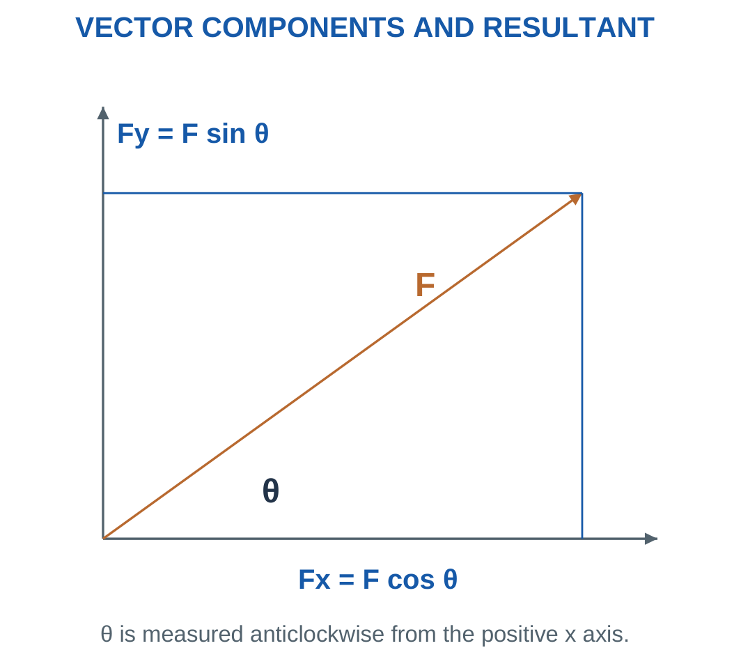
The resultant is the vector sum of forces acting on one body.
Add horizontal components separately from vertical components:
Rx = ΣFx
Ry = ΣFy
Then calculate:
R = √(Rx² + Ry²)
The direction must account for both component signs.

Collinear forces can be added algebraically after choosing a positive direction.
Perpendicular forces use the Pythagorean relation. Arbitrary directions first require component resolution.
A zero resultant force does not automatically mean zero rotational tendency.
Couples
A couple consists of equal opposite parallel forces separated by a perpendicular distance.
Its resultant force is zero, but its moment is nonzero.
For general planar equilibrium, both net force and net moment must vanish.
A resultant vector also needs an appropriate line of action if it is to preserve the moment of the original force system.
Worked Problem 1.9: Resultant from Positive Components
Problem: The force sums are ΣFx = 60 N and ΣFy = 80 N. Find magnitude, direction and balancing-force components.
Step 1:
Rx = 60 N
Ry = 80 N
Step 2:
R = √(60² + 80²) = 100 N
Step 3:
θ = atan2(80, 60) = 53.1301°
The angle is measured from positive x.
Step 4: The balancing force has components:
Fx,balance = −60 N
Fy,balance = −80 N
Its position must still be appropriate for moment balance.
Worked Problem 1.10: Resultant in the Second Quadrant
Problem: ΣFx = −120 N and ΣFy = 50 N.
Step 1:
Rx = −120 N
Ry = 50 N
Step 2:
R = √(120² + 50²) = 130 N
Step 3:
θ = atan2(50, −120) = 157.38°
Step 4: The balancing-force components are:
+120 N horizontally
−50 N vertically
Using an ordinary inverse tangent without quadrant interpretation could give an incorrect direction.
5. Free-Body Diagrams and Support Reactions
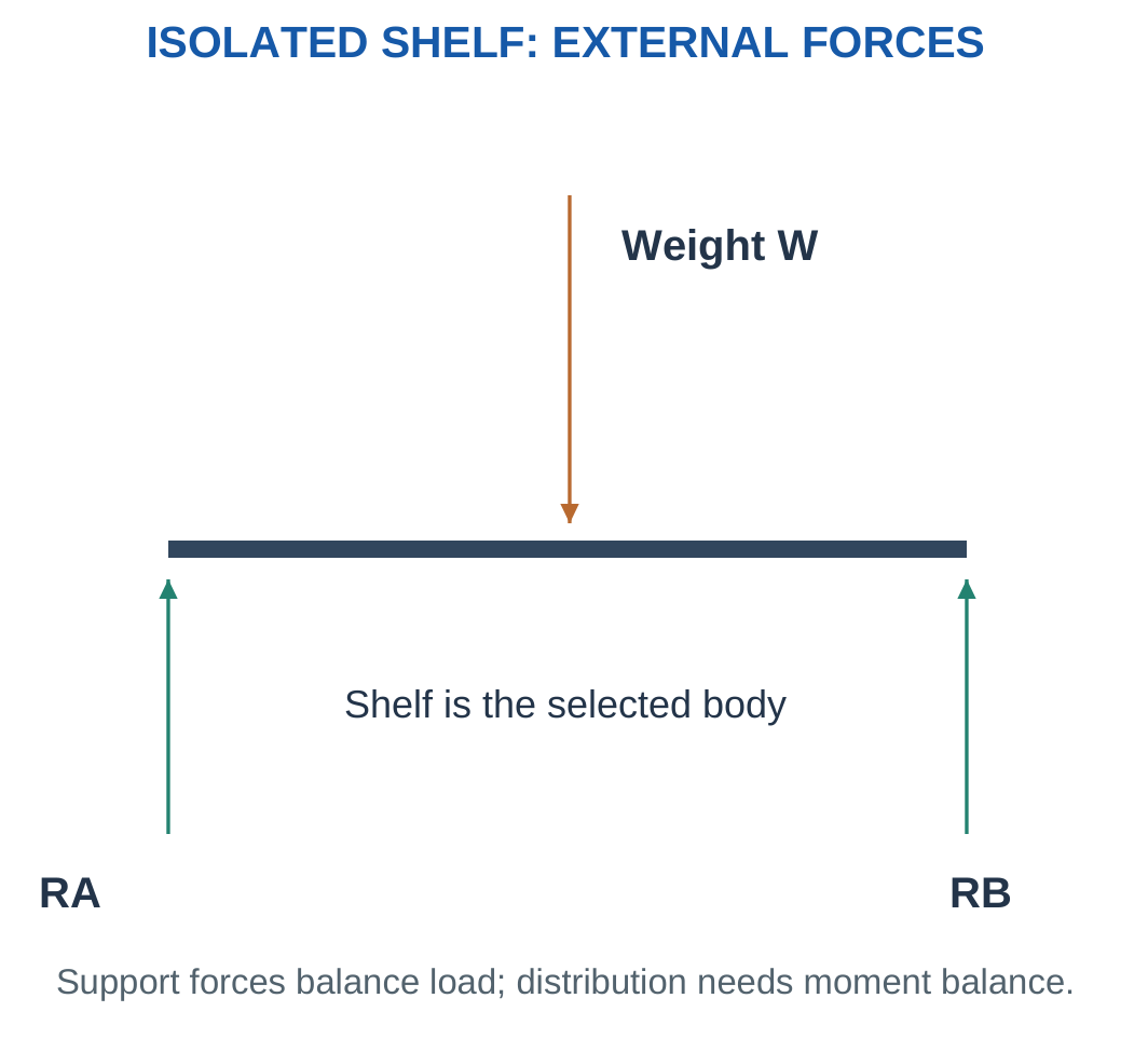
A free-body diagram isolates one selected body and replaces its external contacts by the forces or moments they apply.
Include the body, supplied loads, its weight when included, support reactions and dimensions needed for moments.

Drawing Method
- Select the body.
- State whether its own weight is included.
- Draw an appropriate outline or centreline.
- Replace supports by their allowed reaction components.
- Add supplied forces, couples and dimensions.
- Select axes and moment sign convention.
- Interpret negative answers after solving.
A frictionless roller on a horizontal surface supplies a vertical normal reaction.
An ideal planar pin supplies horizontal and vertical force components but no resisting couple.
An ideal fixed support can supply horizontal force, vertical force and a reaction moment.
Action and Reaction
If a shelf pushes down on a support, the support pushes up on the shelf.
On the shelf’s free-body diagram, show the support’s force on the shelf.
Drawing both action and reaction on the same isolated body incorrectly cancels an interaction that belongs to two different bodies.
A label leader identifies a feature. It should not be interpreted as an additional force arrow.
Worked Problem 1.11: Bracket Support Components
Problem: A bracket carries 400 N downward and 100 N rightward. Find the support-force components for translational equilibrium and state what is needed for the support moment.
Step 1: Choose right and up positive.
Rx + 100 = 0
Rx = −100 N
Step 2:
Ry − 400 = 0
Ry = 400 N
Step 3:
R = √(100² + 400²) = 412.311 N
It is not 500 N.
Step 4: The support moment requires the force lever arms. A fixed support can supply a moment; an ideal pin cannot be assigned one simply to complete an equation.
Worked Problem 1.12: Another Bracket
Problem: A bracket carries 250 N downward and 60 N rightward.
Step 1:
Rx + 60 = 0
Rx = −60 N
Step 2:
Ry − 250 = 0
Ry = 250 N
Step 3:
R = √(60² + 250²) = 257.099 N
Step 4: Lever arms are still required to determine the reaction moment. Force balance alone does not establish rotational equilibrium.
6. Moments, Couples and Lever Arms
A force can turn a body about a reference point.
Moment magnitude is:
M = Fdperp
The distance dperp is perpendicular to the force’s line of action. It is not necessarily the direct distance to the application point.

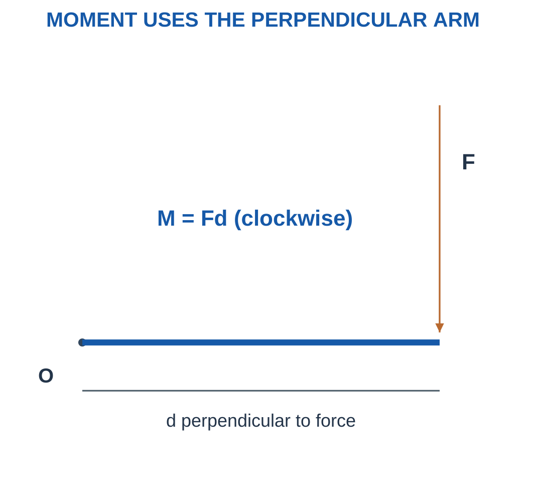
Choose a sign convention, such as counter-clockwise positive.
For a force at position (x, y):
M = xFy − yFx
A force passing through the reference point has zero moment about that point.
Couple Moment
For equal opposite parallel forces separated by perpendicular distance d:
Mcouple = Fd
The distance is the complete separation between the force lines. It should not be counted twice.
A couple moment is independent of the reference point in the rigid-body model.
Units
Force in N multiplied by distance in m gives N·m.
A moment is not a force and cannot be added directly to a force sum.
Torque and bending moment share dimensions but describe their particular loading roles.
Worked Problem 1.13: Moment of a 100 N Force
Problem: A downward 100 N force acts to the right of a pivot at perpendicular distance 0.25 m.
Step 1:
M = 100 × 0.25 = 25 N·m
Step 2: The turning sense is clockwise.
With counter-clockwise positive:
M = −25 N·m
Step 3: An opposing couple for rotational balance is:
+25 N·m
Step 4: The couple balances moment, not the force itself. A support force is also required for translational equilibrium.
Worked Problem 1.14: Moment of a 250 N Force
Problem: A downward 250 N force acts 0.4 m to the right of a pivot.
Step 1:
M = 250 × 0.4 = 100 N·m
Step 2:
Signed moment = −100 N·m
Step 3:
Balancing couple = +100 N·m
Step 4: A separate upward support force is needed to balance the downward load. Moment and force equations must both be satisfied.
Worked Problem 1.15: Moment of an 80 N Force
Problem: An 80 N downward force acts at perpendicular distance 0.15 m.
Step 1:
M = 80 × 0.15 = 12 N·m
Step 2: Its clockwise signed moment is:
−12 N·m
Step 3: The opposing couple is:
+12 N·m
Step 4: Rotational balance does not automatically establish translational balance.
Worked Problem 1.16: Moment from Force Components
Problem: Fx = 40 N and Fy = −100 N act at x = 0.3 m and y = 0.2 m from a reference point.
Step 1: Vertical-component contribution:
xFy = 0.3 × (−100) = −30 N·m
Step 2: Horizontal-component contribution:
−yFx = −0.2 × 40 = −8 N·m
Step 3:
M = −30 − 8 = −38 N·m
Step 4: The result is clockwise. The straight-line distance √(x² + y²) cannot replace the perpendicular arm without the appropriate included angle.
7. Static Equilibrium and Load Sharing
For a planar rigid body in static equilibrium:
ΣFx = 0
ΣFy = 0
ΣM = 0
These equations determine simple support reactions when geometry and support constraints provide sufficient information.

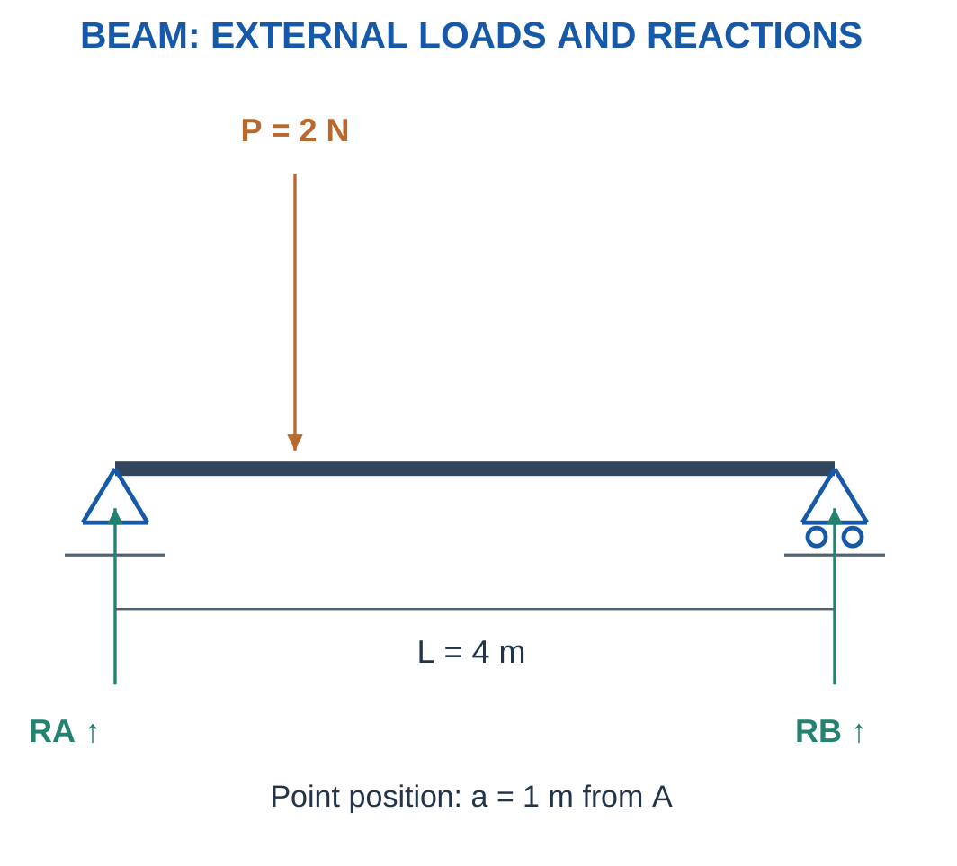
For a simply supported beam of span L with downward load W at distance a from A:
RB L = Wa
Therefore:
RB = Wa/L
RA = W − RB
For a central load and symmetric support conditions:
RA = RB = W/2
An off-centre load is carried more heavily by the nearer support.
Self-Weight and Contact Assumptions
Beam weight is neglected unless supplied or included in another load.
A negative calculated reaction means the actual direction opposes the assumed arrow.
A unilateral contact may not be able to pull. A negative reaction can therefore indicate loss of contact rather than an automatically valid reaction.
Worked Problem 1.17: Central Point Load

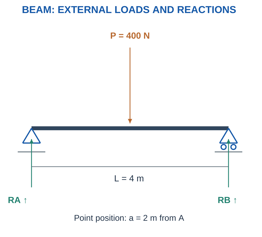
Problem: Find both reactions, neglecting beam weight.
Step 1:
RA + RB = 400 N
Step 2: Take moments about A.
RB × 4 − 400 × 2 = 0
Step 3:
RB = 200 N
RA = 200 N
Step 4: Check moments about B.
RA × 4 = 400 × 2 = 800 N·m
The equal reactions agree with symmetry.
Worked Problem 1.18: Load Nearer the Left Support
Problem: A 3 m span carries 600 N at 1 m from A.
Step 1:
RA + RB = 600 N
Step 2:
RB × 3 = 600 × 1
Step 3:
RB = 200 N
RA = 400 N
Step 4:
RA × 3 = 600 × 2 = 1200 N·m
The nearer left support carries more load.
Worked Problem 1.19: Load Nearer the Right Support
Problem: A 5 m span carries 1000 N at 3 m from A.
Step 1:
RA + RB = 1000 N
Step 2:
RB × 5 = 1000 × 3
Step 3:
RB = 600 N
RA = 400 N
Step 4:
RA × 5 = 1000 × 2 = 2000 N·m
The larger reaction occurs at B, which is closer to the load.
Worked Problem 1.20: Shorter Span
Problem: A 2 m span carries 300 N at 0.5 m from A.
Step 1:
RA + RB = 300 N
Step 2:
RB × 2 = 300 × 0.5
Step 3:
RB = 75 N
RA = 225 N
Step 4:
RA × 2 = 300 × 1.5 = 450 N·m
The force and moment checks both agree.
8. Stress: Internal Force Intensity
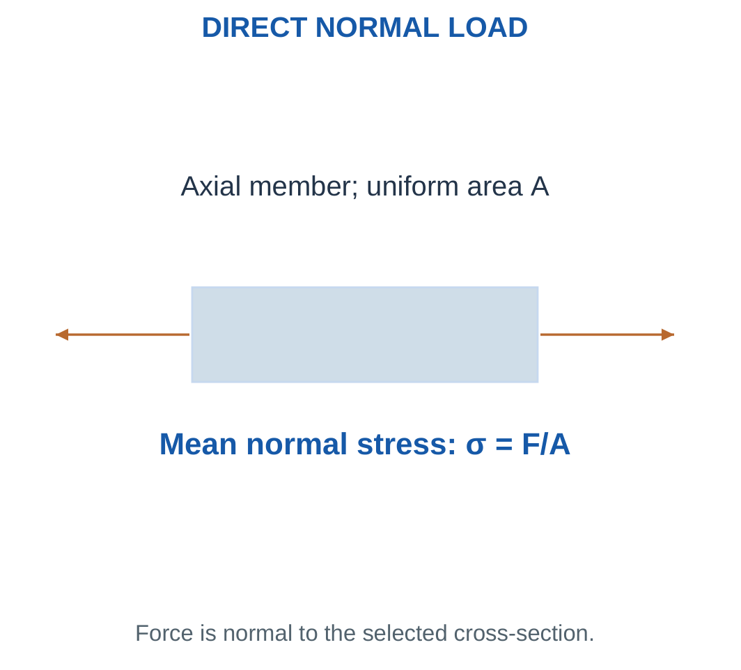
Average normal stress is axial force divided by resisting cross-sectional area:
σ = F/A
Tensile normal stress acts perpendicular to a cut and tends to separate material.
Compressive normal stress acts perpendicular to the cut and tends to push material together.

Using N and mm² gives N/mm², equal to MPa.
Using N and m² gives Pa.
1 MPa = 10⁶ Pa
The average model assumes the load is carried centrally through the selected section. It does not describe local concentrations at holes, notches or abrupt changes.
Force and Stress
A 1000 N load is a force. It is not “1000 N stress.”
Two members carrying the same force can have different stresses because their areas differ.
For a solid circular section:
A = πd²/4
For a hollow circular section:
A = π(D² − d²)/4
Use material cross-sectional area, rather than the exposed side surface.
Worked Problem 1.21: Average Stress in 200 mm²
Problem: A central force of 10000 N is carried by 200 mm².
Step 1:
σ = 10000/200 = 50 N/mm²
Step 2:
σ = 50 MPa
Step 3: Convert area to SI.
A = 0.0002 m²
σ = 10000/0.0002 = 5 × 10⁷ Pa
Step 4: The result is an average intensity. Tension or compression follows the loading direction; local concentrations or buckling need additional information.
Worked Problem 1.22: Average Stress in 120 mm²
Problem: A 6000 N central force acts through 120 mm².
Step 1:
σ = 6000/120 = 50 N/mm²
Step 2:
σ = 50 MPa
Step 3:
A = 0.00012 m²
σ = 5 × 10⁷ Pa
Step 4: The same stress as the previous problem occurs because force and area have changed in the same proportion.
Worked Problem 1.23: Average Stress in 300 mm²
Problem: A central force of 18000 N acts through 300 mm².
Step 1:
σ = 18000/300 = 60 N/mm²
Step 2:
σ = 60 MPa
Step 3:
A = 0.0003 m²
σ = 6 × 10⁷ Pa
Step 4: The selected area and central-loading assumption define the average. A complete component assessment may require other loading modes.
Worked Problem 1.24: Average Stress in 50 mm²
Problem: A central force of 2500 N acts through 50 mm².
Step 1:
σ = 2500/50 = 50 N/mm²
Step 2:
σ = 50 MPa
Step 3:
A = 5 × 10⁻⁵ m²
σ = 5 × 10⁷ Pa
Step 4: A smaller force does not necessarily mean smaller stress. The resisting area must also be considered.
9. Tension, Compression and Simple Shear
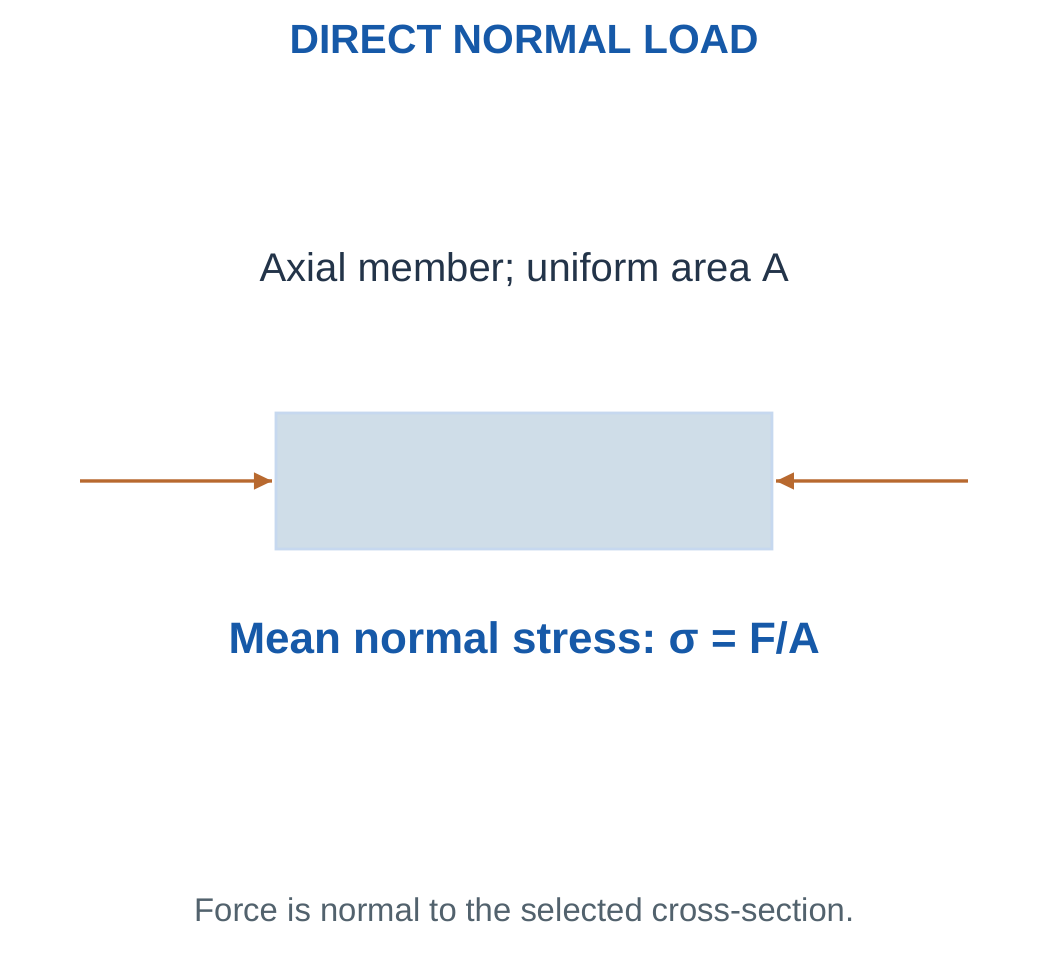
For a centrally loaded axial member, direct normal-stress magnitude is F/A.
Tension and compression can be assigned opposite signs when a convention is stated. Many introductory questions request a positive magnitude while identifying the load type separately.

Average simple shear stress is:
τ = V/Ashear
For an ideal double-shear pin with two equally loaded planes:
Ashear,total = 2Aplane
The planes must be specified. A bolted connection is not automatically a double-shear model.
Compression and Buckling
A short compression block may be treated using average direct stress.
A slender compressed member can fail by buckling before reaching a simple crushing-stress limit.
A direct-stress calculation does not by itself establish slender-member stability.
Joint Limitations
Real joints can require bearing, bending, preload, fatigue and edge-distance checks.
The numerical examples use stated uniform shear or direct-load models to practise stress.
Equal load division among several members requires symmetry or an explicit assumption.
Worked Problem 1.25: Single-Shear Pin
Problem: A 10 mm pin carries 5000 N on one uniform resisting shear plane.
Step 1:
Aplane = π × 10²/4 = 78.5398 mm²
Step 2:
Ashear = 78.5398 mm²
Step 3:
τ = 5000/78.5398 = 63.662 MPa
Step 4: The plane count is one. No double-shear factor is introduced unless the geometry and model specify a second equally loaded plane.
Worked Problem 1.26: Double-Shear Pin
Problem: A 12 mm pin carries 12000 N through two equally loaded resisting planes.
Step 1:
Aplane = π × 12²/4 = 113.097 mm²
Step 2:
Ashear,total = 2 × 113.097 = 226.195 mm²
Step 3:
τ = 12000/226.195 = 53.0516 MPa
Step 4: Equivalently, each plane carries 6000 N. Dividing 6000 N by one plane’s area gives the same stress.
Worked Problem 1.27: Larger Single-Shear Pin
Problem: A 16 mm pin carries 8000 N on one plane.
Step 1:
Aplane = π × 16²/4 = 201.062 mm²
Step 2:
Ashear = 201.062 mm²
Step 3:
τ = 8000/201.062 = 39.7887 MPa
Step 4: This is an average shear result. Bearing or bending in a real connection would require separate information.
Worked Problem 1.28: Hollow Round Member
Problem: Outside diameter is 30 mm, inside diameter is 20 mm and central axial force is 15000 N.
Step 1:
Aouter = π × 30²/4 = 706.858 mm²
Step 2:
Avoid = π × 20²/4 = 314.159 mm²
Step 3:
A = 706.858 − 314.159 = 392.699 mm²
Step 4:
σ = 15000/392.699 = 38.1972 MPa
Using the outer circle alone would overstate the material area and understate stress.
10. Strain and Dimensional Change
Engineering normal strain is:
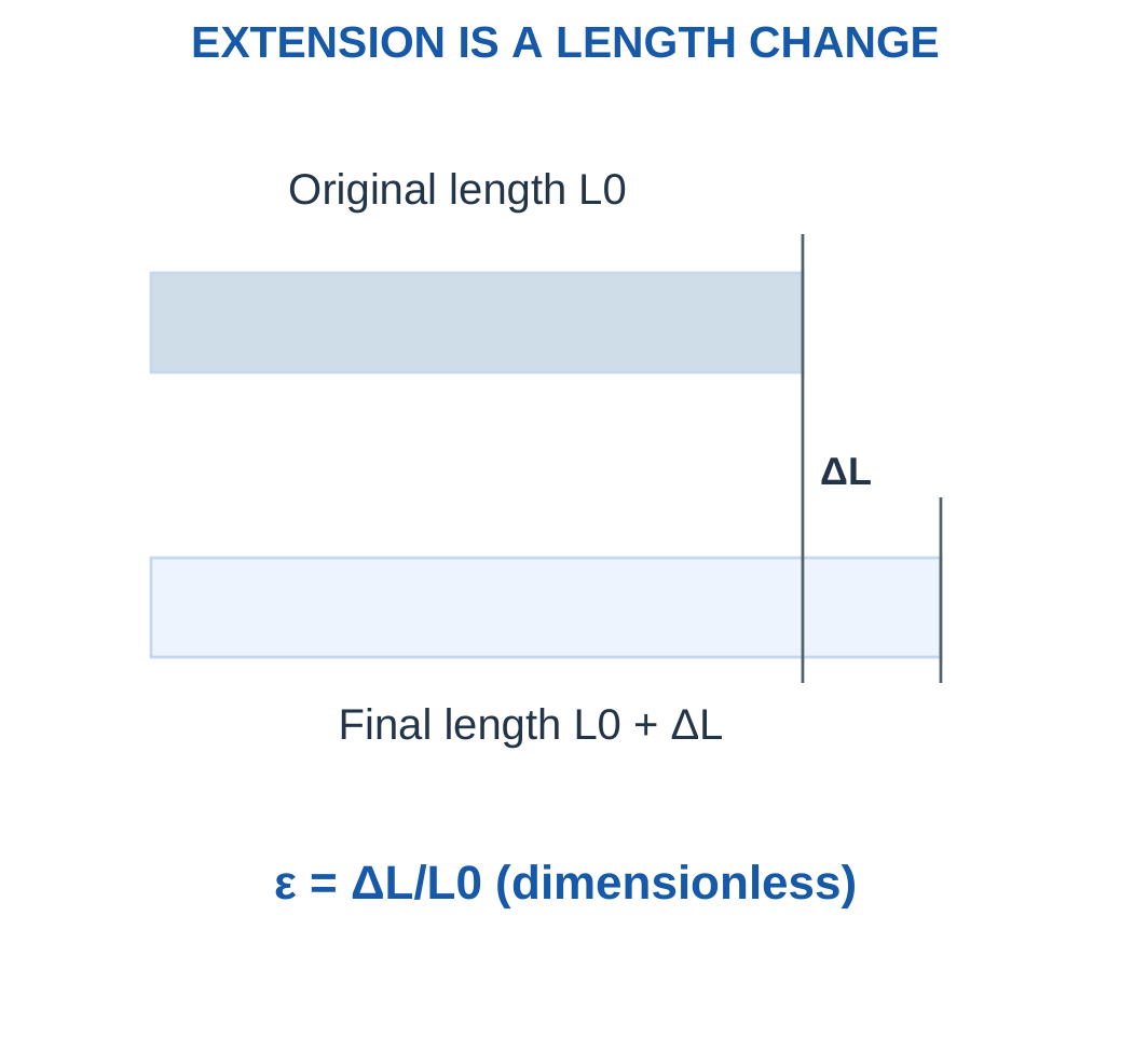
ε = ΔL/L0
It is dimensionless because the numerator and denominator use the same length unit.
Extension is positive under the usual tensile convention. Shortening can be represented by a negative value.

A small strain can be written as a decimal, percentage or microstrain.
0.001 = 0.1% = 1000 microstrain
Decimal-to-percent conversion multiplies by 100.
Decimal-to-microstrain conversion multiplies by 10⁶.
Unit Consistency
An extension in mm and an original length in m cannot be divided as bare numbers.
Convert both lengths to mm or both to m first.
The final length is L0 + ΔL, but engineering strain retains L0 in its denominator.
Recovery and Permanence
Strain is not automatically permanent deformation.
A component can recover after unloading within its elastic range. Whether a measured strain is elastic, plastic or partly both depends on the material response.
Worked Problem 1.29: Strain from 0.2 mm Extension
Problem: Original gauge length is 200 mm and extension is 0.2 mm.
Step 1:
ε = 0.2/200 = 0.001
Step 2:
Percentage strain = 0.001 × 100 = 0.1%
Step 3:
Microstrain = 0.001 × 10⁶ = 1000
Step 4:
Final length = 200 + 0.2 = 200.2 mm
The final length is not substituted into the engineering-strain denominator.
Worked Problem 1.30: Strain from 0.15 mm Extension
Problem: Original length is 500 mm and extension is 0.15 mm.
Step 1:
ε = 0.15/500 = 0.0003
Step 2:
Percentage strain = 0.03%
Step 3:
Microstrain = 300
Step 4:
Final length = 500.15 mm
All three strain representations describe the same dimensionless ratio.
Worked Problem 1.31: Strain from 0.8 mm Extension
Problem: Original length is 1000 mm and extension is 0.8 mm.
Step 1:
ε = 0.8/1000 = 0.0008
Step 2:
Percentage strain = 0.08%
Step 3:
Microstrain = 800
Step 4:
Final length = 1000.8 mm
The consistent use of original length distinguishes engineering strain from other possible deformation measures.
11. Elasticity, Hooke’s Law and Young’s Modulus
Elastic deformation is recoverable when load is removed.
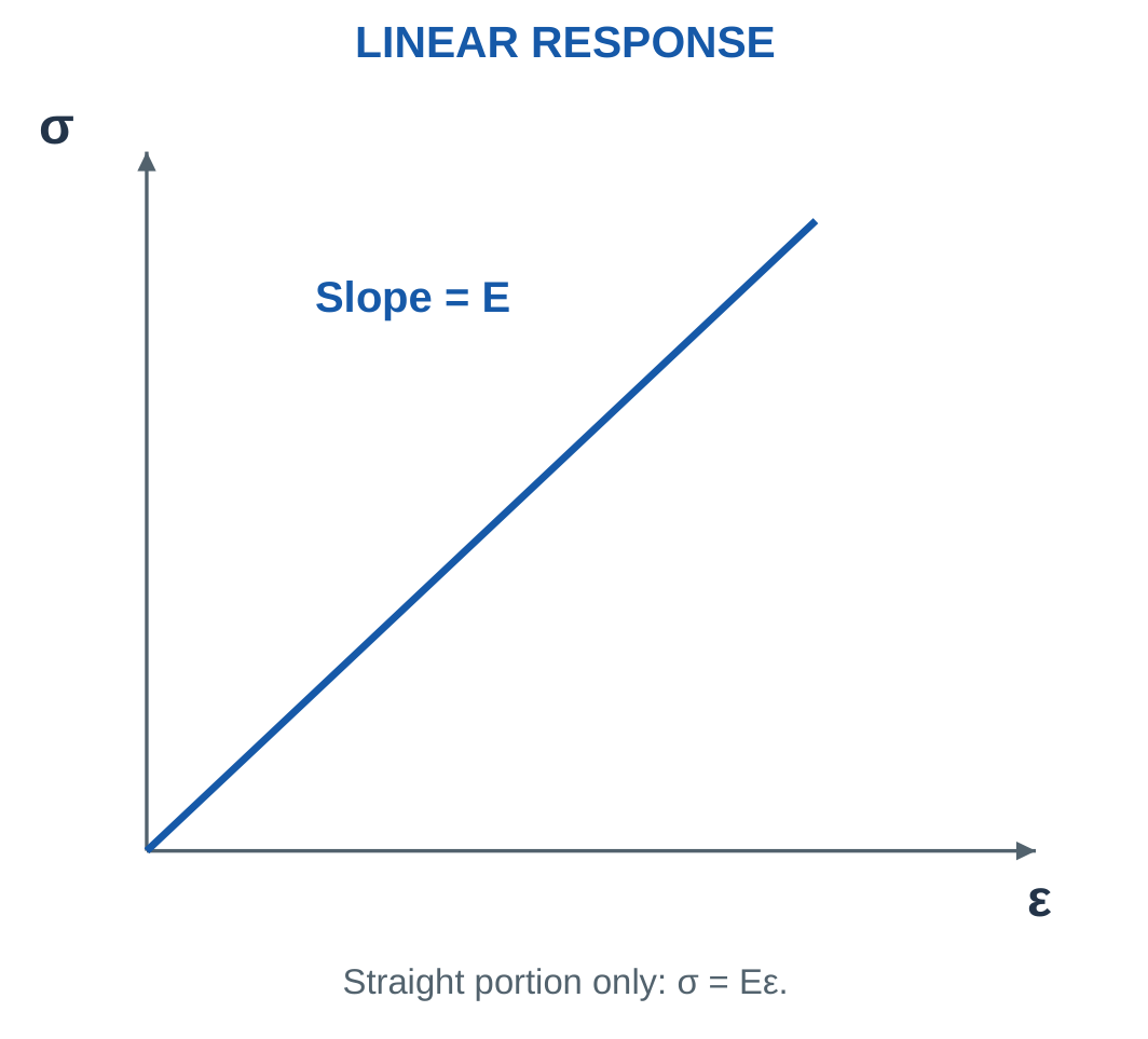
Within a linear-elastic uniaxial range:
σ = Eε
Young’s modulus E is the stress-strain slope in that range and has the same units as stress.

Combining:
σ = F/A
and:
ε = ΔL/L
gives:
ΔL = FL/(AE)
for a uniform straight bar under central axial loading.
Material Modulus and Member Stiffness
E is a material parameter.
The complete member’s axial stiffness is:
k = AE/L
It depends on material and geometry.
A high modulus means less elastic strain for a given uniaxial stress. It does not by itself establish high failure strength, impact resistance or minimum mass.
Modulus Units
If stress is in MPa, express E in MPa.
200 GPa = 200000 MPa
Using the numerical value 200 with stress in MPa would create a thousandfold error.
Do not extend a straight-line formula into a plastic range without a supplied model.
Worked Problem 1.32: Steel-Like Supplied Modulus
Problem: L = 500 mm, A = 200 mm², E = 200 GPa and F = 10000 N. The stated response is linear elastic.
Step 1:
E = 200000 MPa
σ = 10000/200 = 50 MPa
Step 2:
ε = 50/200000 = 0.00025
Step 3:
ΔL = 0.00025 × 500 = 0.125 mm
Step 4:
k = 200 × 200000/500 = 80000 N/mm
Check:
kΔL = 80000 × 0.125 = 10000 N
Worked Problem 1.33: Supplied Modulus of 70 GPa
Problem: L = 400 mm, A = 150 mm², E = 70 GPa and F = 6000 N.
Step 1:
E = 70000 MPa
σ = 6000/150 = 40 MPa
Step 2:
ε = 40/70000 = 0.000571429
Step 3:
ΔL = 0.000571429 × 400 = 0.228571 mm
Step 4:
k = 150 × 70000/400 = 26250 N/mm
The force check gives approximately 6000 N.
Worked Problem 1.34: Supplied Modulus of 120 GPa
Problem: L = 600 mm, A = 300 mm², E = 120 GPa and F = 12000 N.
Step 1:
E = 120000 MPa
σ = 12000/300 = 40 MPa
Step 2:
ε = 40/120000 = 0.000333333
Step 3:
ΔL = 0.000333333 × 600 = 0.2 mm
Step 4:
k = 300 × 120000/600 = 60000 N/mm
Check:
60000 × 0.2 = 12000 N
Worked Problem 1.35: Lower-Modulus Member
Problem: L = 250 mm, A = 100 mm², E = 3 GPa and F = 3000 N. The stated linear range applies.
Step 1:
E = 3000 MPa
σ = 3000/100 = 30 MPa
Step 2:
ε = 30/3000 = 0.01
Step 3:
ΔL = 0.01 × 250 = 2.5 mm
Step 4:
k = 100 × 3000/250 = 1200 N/mm
Check:
1200 × 2.5 = 3000 N
The calculation follows the explicitly supplied linear model.
12. Reading a Stress–Strain Curve
A stress-strain curve relates measured stress and strain during loading.
The initial linear region gives modulus.
Yielding marks the onset of significant plastic deformation under the chosen definition.
Ultimate tensile strength is the maximum engineering stress reached in the tensile test.


Fracture is final separation.
In a ductile tensile test, engineering stress can fall after the maximum as necking develops while original area remains in the definition.
This does not mean the specimen becomes unstressed.
Brittle materials often show little plastic strain before fracture. Not every material has a clear yield plateau or an identical curve shape.
Engineering and True Definitions
This unit mainly uses force divided by original area and extension divided by original length.
Changing those definitions gives other measures. They should not be mixed inside one interpretation without explanation.
A load-extension graph includes specimen geometry. A stress-strain graph is more directly a material-response representation.
Worked Problem 1.36: Modulus from Two Graph Points
Problem: A straight elastic segment contains points (0.0002, 40 MPa) and (0.0004, 80 MPa). Find E and strain at 120 MPa if the same line is explicitly valid there.
Step 1:
Δσ = 80 − 40 = 40 MPa
Δε = 0.0004 − 0.0002 = 0.0002
Step 2:
E = 40/0.0002 = 200000 MPa = 200 GPa
Step 3:
ε = 120/200000 = 0.0006
Step 4: Extrapolation beyond the stated elastic range would require more response information. The initial slope does not determine every yield or fracture point.
Worked Problem 1.37: Another Linear Segment
Problem: A straight segment contains (0.0005, 35 MPa) and (0.001, 70 MPa). Find E and strain at 105 MPa where the line remains valid.
Step 1:
Δσ = 35 MPa
Δε = 0.0005
Step 2:
E = 35/0.0005 = 70000 MPa = 70 GPa
Step 3:
ε = 105/70000 = 0.0015
Step 4: The result depends on the supplied validity of the line at 105 MPa. It is not an unrestricted material law.
13. Material Properties That Must Not Be Confused
Stiffness concerns resistance to elastic deformation.
Strength concerns the stress associated with a specified limiting event, such as yield or fracture.
Hardness concerns resistance to local indentation or scratching under a stated test.
Toughness concerns energy absorbed before fracture under the relevant test and loading condition.

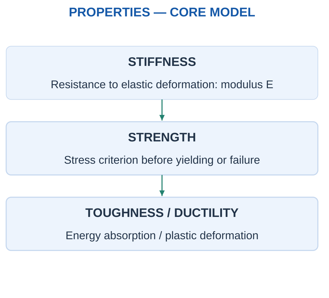
Ductility describes plastic deformation capacity before fracture.
Brittleness indicates relatively little plastic deformation before fracture under the stated condition.
Elasticity describes recovery, rather than simply being easy to stretch.
Property Comparison
| Property | Question Answered |
|---|---|
| Modulus | How much elastic strain occurs for a given stress? |
| Strength | What stress limit is relevant? |
| Ductility | How much plastic deformation occurs before fracture? |
| Toughness | How much energy can be absorbed before breaking? |
| Density | What mass corresponds to a given volume? |
| Corrosion resistance | How does the material withstand its environment? |
A ceramic can be stiff and brittle. A polymer can show large recoverable strain while having a lower modulus than a metal.
Property values depend on grade, processing, temperature, loading rate, direction and test conditions.
Worked Problem 1.38: Stiffness and Strength Rankings
Problem: Candidate A has E = 200 GPa and strength limit 250 MPa. B has E = 70 GPa and strength limit 300 MPa. Compare strains at 30 MPa in their stated linear ranges.
Step 1:
εA = 30/200000 = 0.00015
Step 2:
εB = 30/70000 = 0.000428571
A is stiffer.
Step 3: B has the higher stated strength limit, 300 MPa compared with 250 MPa.
Step 4:
εB/εA = 200/70 = 2.85714
The stiffness ranking differs from the strength ranking. Neither establishes impact toughness or minimum component mass.
Worked Problem 1.39: Another Property Comparison
Problem: EA = 120 GPa, EB = 60 GPa, SA = 180 MPa and SB = 360 MPa. Compare strains at 30 MPa.
Step 1:
εA = 30/120000 = 0.00025
Step 2:
εB = 30/60000 = 0.0005
A is stiffer.
Step 3: B has the higher supplied strength limit.
Step 4:
εB/εA = 2
A higher modulus does not automatically imply a higher failure stress.
Worked Problem 1.40: Lower-Modulus Candidates
Problem: EA = 5 GPa, EB = 2 GPa, SA = 60 MPa and SB = 80 MPa. Compare at 30 MPa in the stated linear ranges.
Step 1:
εA = 30/5000 = 0.006
Step 2:
εB = 30/2000 = 0.015
A is stiffer.
Step 3: B has the higher stated strength limit.
Step 4:
εB/εA = 2.5
The result illustrates why stiffness and strength must be assessed separately.
14. Simple Allowable-Stress and Stiffness Checks
A basic direct-load check compares average working stress with a supplied allowable stress.
If:
F/A ≤ σallow
the stated average direct-stress criterion passes.
This does not establish every possible failure mode.
If strength S and factor n are explicitly supplied:
σallow = S/n
may be the question’s chosen definition. Use that supplied definition rather than inventing a universal factor.

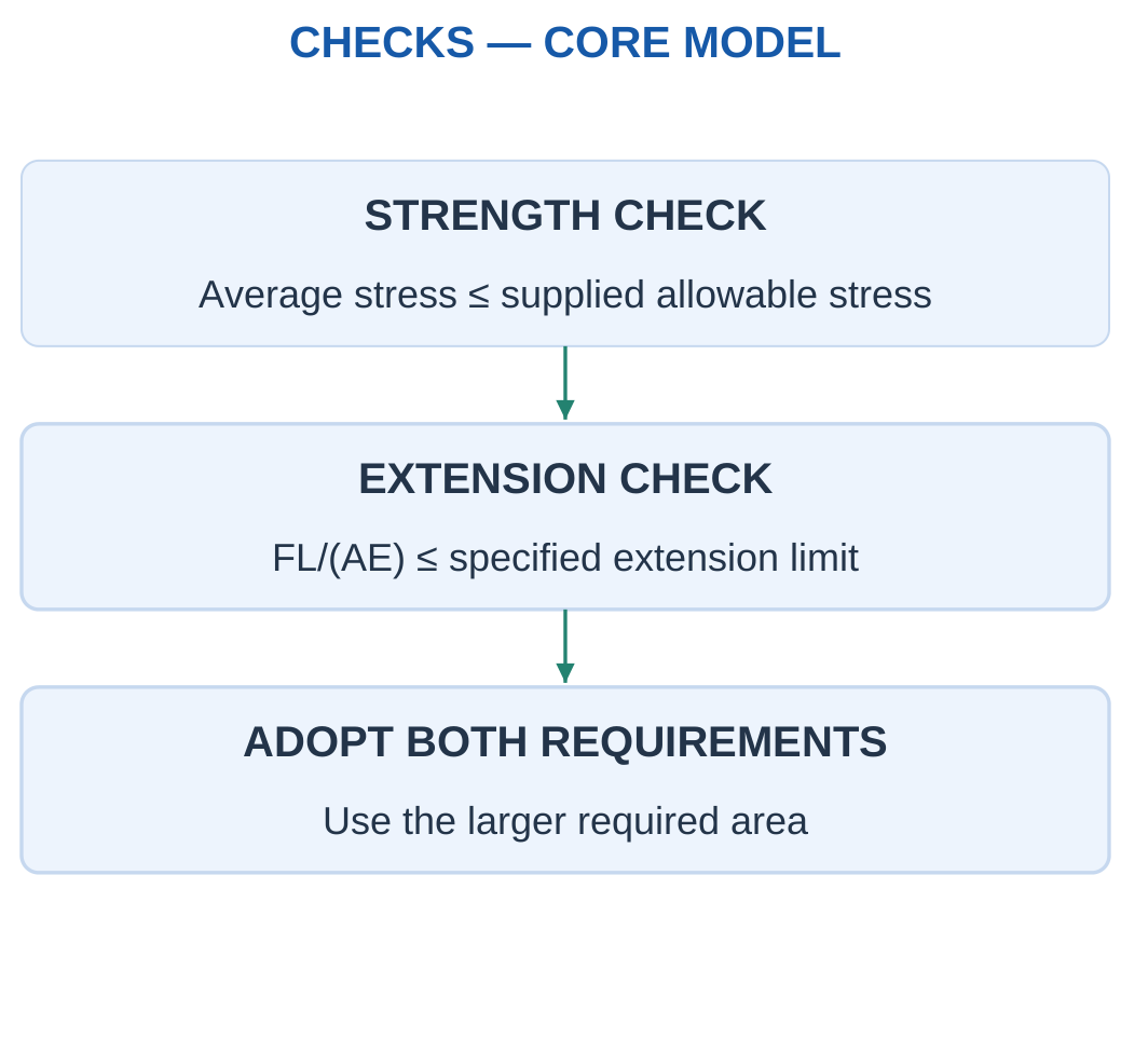
The stress-based minimum area is:
A ≥ F/σallow
For an extension limit:
A ≥ FL/(EΔLmax)
The larger area requirement controls these two constraints.
Rounding
A minimum dimension must not be rounded downward if that violates the inequality.
After selecting a practical dimension, recalculate actual stress or extension.
Local stress, buckling, joints, fatigue and service conditions remain separate considerations.
Worked Problem 1.41: Minimum Round Diameter
Problem: F = 12000 N and allowable average stress is 60 MPa. Find minimum area, ideal diameter and an upward-rounded whole-mm diameter.
Step 1:
Amin = 12000/60 = 200 mm²
Step 2:
dmin = √(4 × 200/π) = 15.9577 mm
Step 3: Choose:
d = 16 mm
Step 4:
σactual = 4F/(πd²) = 59.6831 MPa
It is below 60 MPa under the supplied direct-stress model.
Worked Problem 1.42: Lower Load and Allowable Stress
Problem: F = 8000 N and σallow = 40 MPa.
Step 1:
Amin = 8000/40 = 200 mm²
Step 2:
dmin = 15.9577 mm
Step 3:
Choose d = 16 mm
Step 4:
σactual = 39.7887 MPa
The rounded dimension satisfies the stated 40 MPa criterion.
Worked Problem 1.43: Higher Load and Allowable Stress
Problem: F = 18000 N and σallow = 90 MPa.
Step 1:
Amin = 18000/90 = 200 mm²
Step 2:
dmin = 15.9577 mm
Step 3:
Choose d = 16 mm
Step 4:
σactual = 89.5247 MPa
The same minimum area occurs because the load-to-allowable-stress ratio is unchanged.
Worked Problem 1.44: Stress and Extension Together
Problem: A member carries 10000 N over 500 mm. E = 70000 MPa, allowable stress is 80 MPa and maximum extension is 0.2 mm.
Step 1: Stress requirement:
A ≥ 10000/80 = 125 mm²
Step 2: Extension requirement:
A ≥ 10000 × 500/(70000 × 0.2)
A ≥ 357.143 mm²
Step 3: Choose the larger minimum:
Amin = 357.143 mm²
Step 4: At this area:
σ = 28 MPa
ΔL = 0.2 mm
The extension constraint controls.
15. Beams and Ideal Support Types
A beam is often modelled as a member carrying transverse loading along a span.
The same shelf, rail or arm can require different beam models depending on its actual support and connection behaviour.

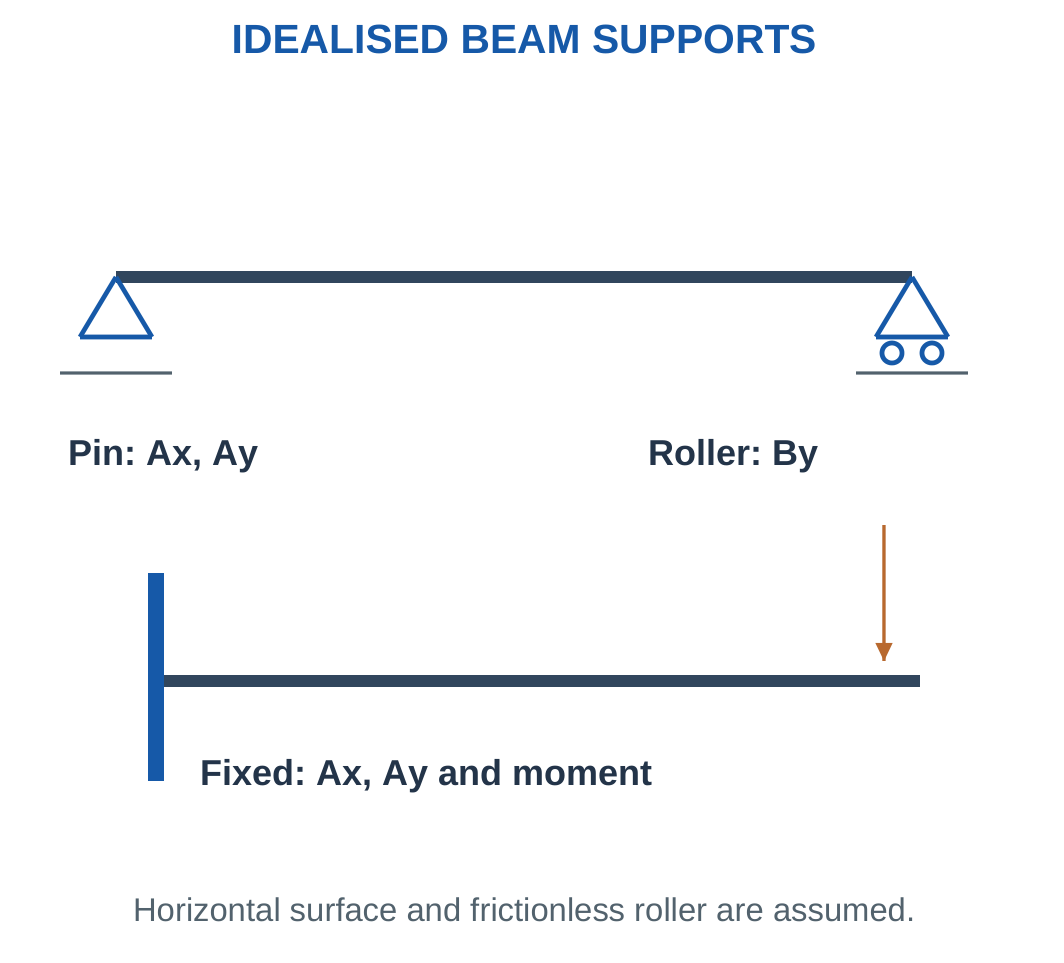
A simply supported beam commonly uses a pin and roller in a planar model.
A cantilever has one fixed end and one free end.
A fixed support resists translation and rotation through force components and a reaction moment.
Beam Diagram Requirements
- Span and support positions.
- Point-load magnitudes and locations.
- Distributed-load intensity and loaded length.
- Applied couples and their senses.
- Self-weight assumption.
- Sign convention.
A real bolted connection is not automatically an ideal fixed support in every direction.
A contact shelf is not automatically capable of sustaining a tensile reaction.
The stated model determines which reactions are available.
Worked Problem 1.45: Simply Supported Midspan Load
Problem: A 2 m simply supported beam carries 300 N at midspan. Find vertical reactions and support moments.
Step 1:
RA + RB = 300 N
Step 2: Symmetry gives:
RA = RB = 150 N
Step 3: Horizontal reaction is zero under the purely vertical load. No fixed-end reaction couple is assigned.
Step 4: The reaction set follows the ideal pin-and-roller constraints. Changing support type changes the model.
Worked Problem 1.46: Cantilever Tip Load
Problem: A 1.5 m cantilever carries 500 N downward at its free end.
Step 1:
Vertical reaction = 500 N upward
Step 2:
Load moment = 500 × 1.5 = 750 N·m
Step 3: The fixed support supplies an opposing 750 N·m couple. Horizontal reaction is zero.
Step 4: An ideal pin alone would not provide this resisting moment. The fixed-end assumption is essential.
Worked Problem 1.47: Larger Midspan Load
Problem: A 3 m simply supported beam carries 800 N at midspan.
Step 1:
RA + RB = 800 N
Step 2:
RA = RB = 400 N
Step 3: No support couple is assigned to the ideal pin or roller under this model.
Step 4: Equal reactions follow from symmetry, rather than merely from the existence of two supports.
16. Point Loads on Simply Supported Beams
A point load idealises a force concentrated at one span location.
Real contact has finite area, but a point resultant can be suitable for external equilibrium when contact length is small compared with span.

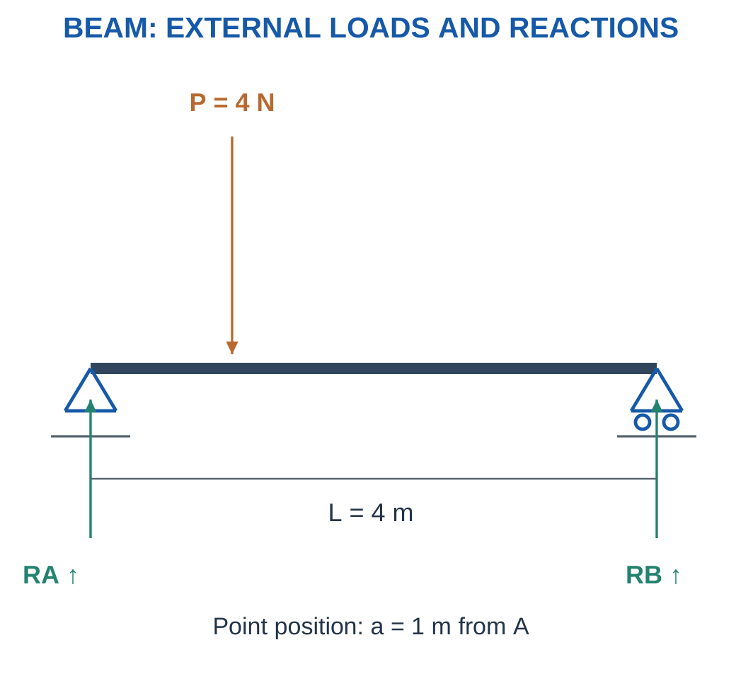
For a load W at distance a from A:
RB = Wa/L
RA = W(L − a)/L
For multiple point loads:
RB L = ΣWi ai
Then:
RA = ΣWi − RB
Physical Check
Move a downward load toward A while keeping load and span fixed.
RA should increase and RB should decrease.
A result showing the opposite suggests exchanged labels or lever arms.
A load on an overhang can produce a negative reaction. Such a result requires interpretation of the actual support and contact capability.
Worked Problem 1.48: 800 N at 1 m

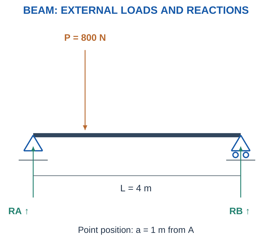
Problem: Find reactions, neglecting beam weight.
Step 1:
RA + RB = 800 N
Step 2:
RB × 4 = 800 × 1
Step 3:
RB = 200 N
RA = 600 N
Step 4:
RA × 4 = 800 × 3 = 2400 N·m
The nearer left support carries more load.
Worked Problem 1.49: 450 N at 2 m


Step 1:
RA + RB = 450 N
Step 2:
RB × 3 = 450 × 2
Step 3:
RB = 300 N
RA = 150 N
Step 4:
RA × 3 = 450 × 1 = 450 N·m
The right support is closer and carries the larger reaction.
Worked Problem 1.50: 1000 N on a 5 m Span
Problem: A 5 m beam carries 1000 N at 2 m from A.
Step 1:
RA + RB = 1000 N
Step 2:
RB × 5 = 1000 × 2
Step 3:
RB = 400 N
RA = 600 N
Step 4:
RA × 5 = 1000 × 3 = 3000 N·m
Both equilibrium checks agree.
Beam and Support Fixture

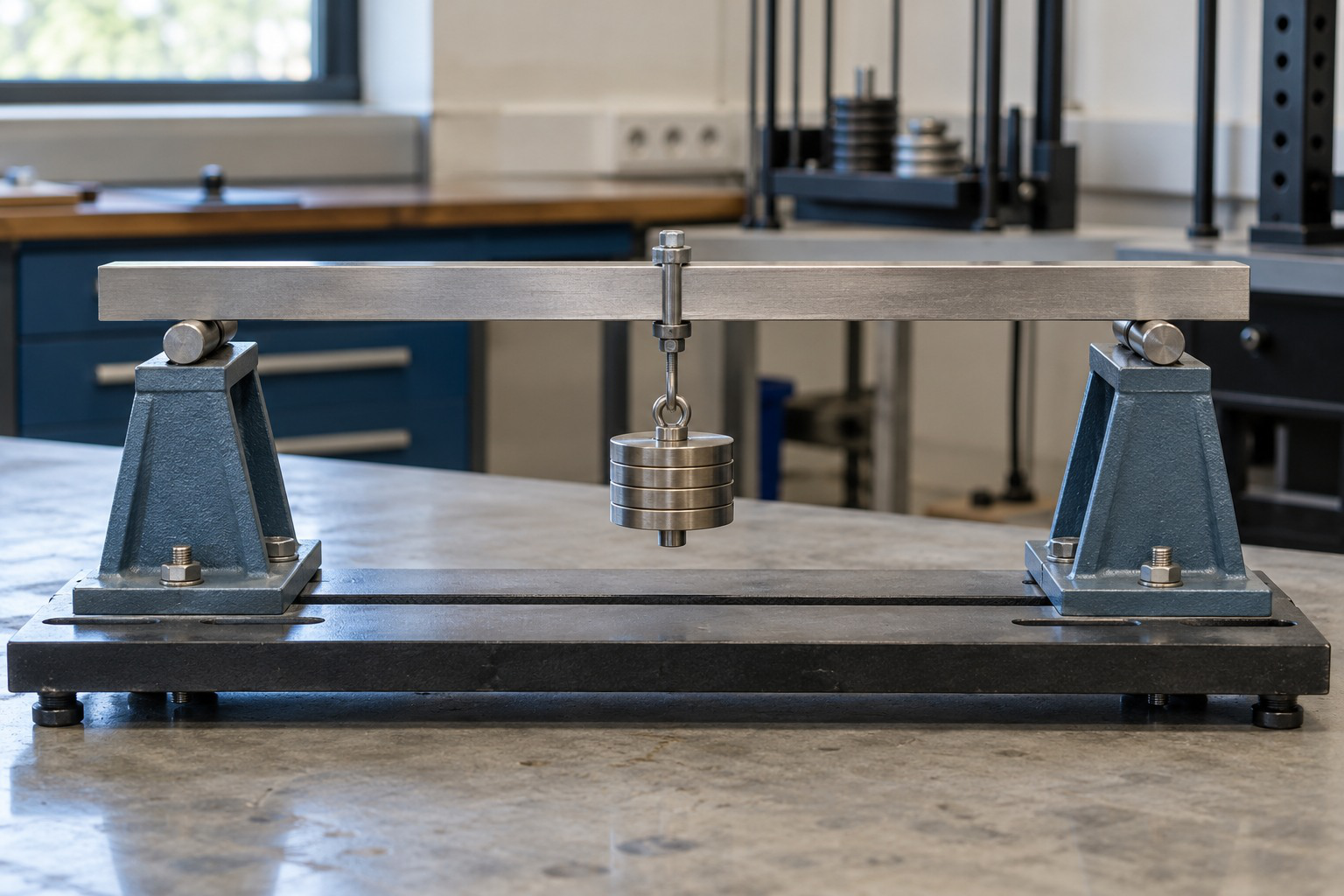
The selected support and loading model determines reactions and bending demand.
A photograph supplies context. Dimensions, constraints and assumptions come from the stated problem.
17. Uniformly Distributed Loads
A uniformly distributed load has constant force per unit length:
w in N/m or kN/m
Over loaded length l:
W = wl
Its equivalent resultant acts at the midpoint of that uniformly loaded segment.

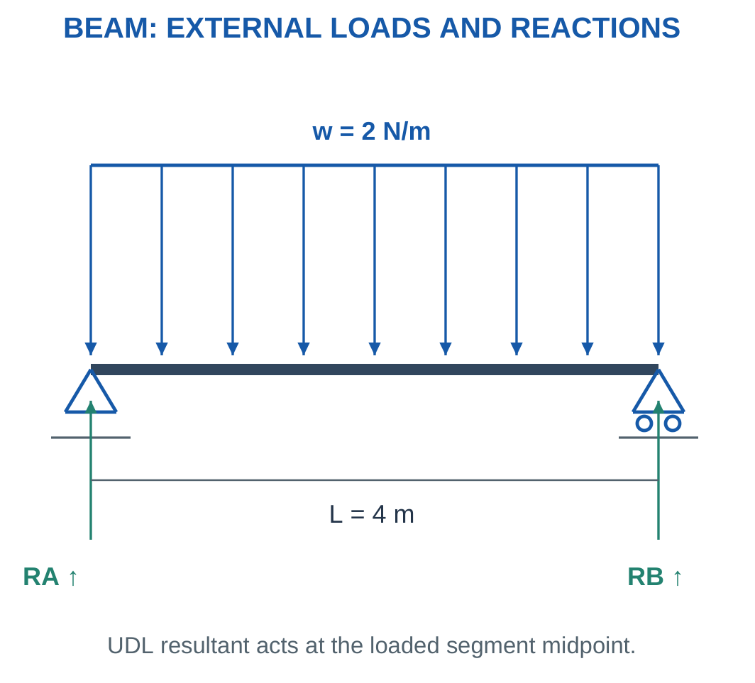
For a full-span UDL on a symmetric simply supported beam:
RA = RB = wL/2
For partial loading, use the midpoint of the loaded segment, not automatically the beam centre.
Intensity and Total Force
A 2 kN/m load over 3 m gives:
W = 2 × 3 = 6 kN
The intensity is not itself a total force.
Replacing a UDL by its resultant preserves total external force and moment for reaction calculations. It does not reproduce every local internal-force or deformation distribution.
Worked Problem 1.51: Full-Span UDL

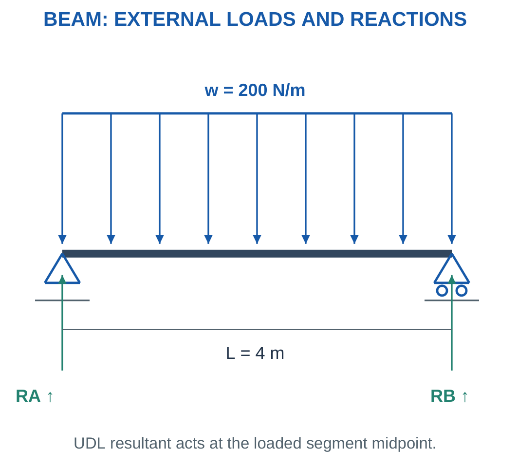
Problem: A 4 m span carries 200 N/m over its full length.
Step 1:
W = 200 × 4 = 800 N
Step 2:
xR = 0 + 4/2 = 2 m
Step 3:
RB = 800 × 2/4 = 400 N
Step 4:
RA = 800 − 400 = 400 N
The force and moment checks agree.
Worked Problem 1.52: Partial UDL

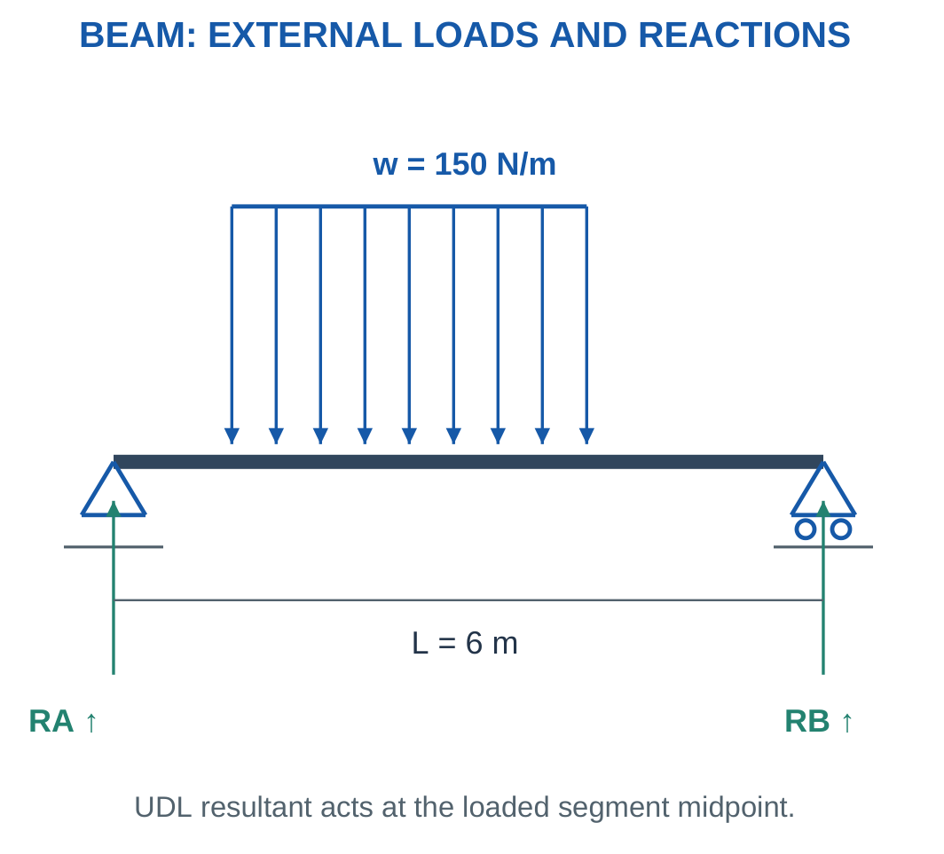
Problem: A 6 m span carries 150 N/m from x = 1 m over 3 m.
Step 1:
W = 150 × 3 = 450 N
Step 2:
xR = 1 + 3/2 = 2.5 m
Step 3:
RB = 450 × 2.5/6 = 187.5 N
Step 4:
RA = 450 − 187.5 = 262.5 N
Using the whole-beam midpoint would give the wrong moment.
Worked Problem 1.53: UDL Beginning at 2 m
Problem: A 5 m span carries 300 N/m over 2 m beginning at x = 2 m.
Step 1:
W = 300 × 2 = 600 N
Step 2:
xR = 2 + 2/2 = 3 m
Step 3:
RB = 600 × 3/5 = 360 N
Step 4:
RA = 600 − 360 = 240 N
The greater right reaction agrees with the resultant lying nearer B.
Worked Problem 1.54: Symmetric Full UDL
Problem: A 3 m span carries 250 N/m over its full length.
Step 1:
W = 250 × 3 = 750 N
Step 2:
xR = 1.5 m
Step 3:
RB = 750 × 1.5/3 = 375 N
Step 4:
RA = 375 N
Equal reactions follow from the full-span symmetric loading.
18. Combined Loads and Cantilever Reactions
A beam can carry point loads and distributed loads together.
For external equilibrium, convert each uniform segment into its own resultant at the correct location.
Then add load moments and solve support reactions.

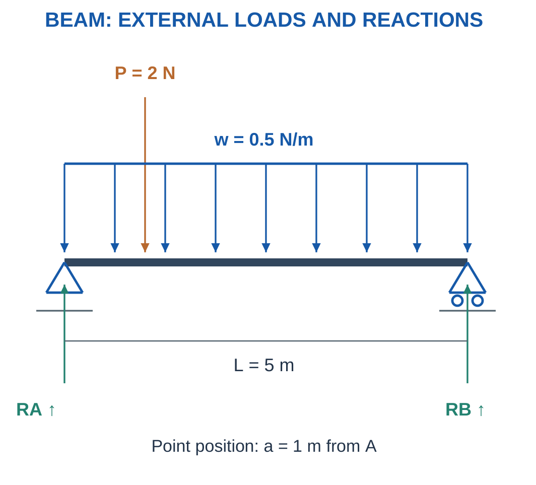
For a cantilever with tip load W:
Vertical reaction = W
Reaction moment magnitude = WL
A full-length UDL adds:
Force = wL
Moment = wL²/2
The reaction couple opposes the net applied turning effect.
Position Information
A 100 N force at 0.2 m produces a different moment from 100 N at 1 m.
Equal total force does not establish equal support moment or equal bending demand.
Worked Problem 1.55: Point Load and Full UDL

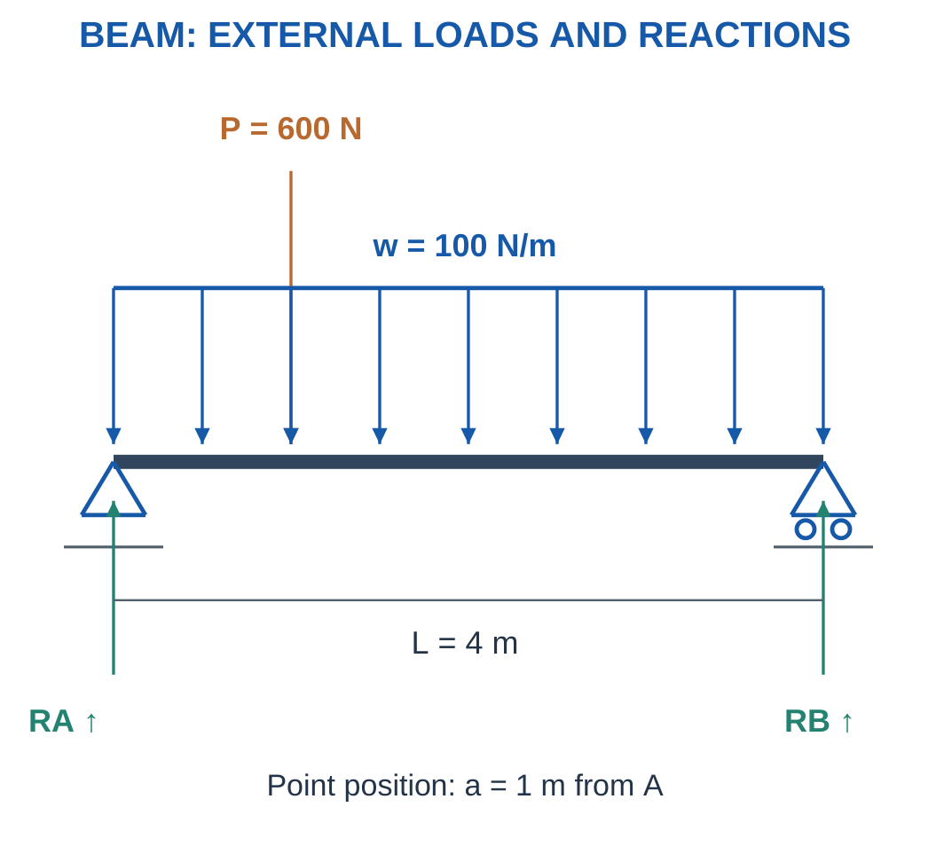
Problem: A 4 m span carries 600 N at x = 1 m and a full-span UDL of 100 N/m.
Step 1:
U = 100 × 4 = 400 N
It acts at x = 2 m.
Step 2:
Total load = 600 + 400 = 1000 N
Step 3:
RB × 4 = 600 × 1 + 400 × 2
RB = 350 N
Step 4:
RA = 1000 − 350 = 650 N
Check about B:
650 × 4 = 600 × 3 + 400 × 2
Worked Problem 1.56: Larger Combined Loading
Problem: A 5 m span carries 1000 N at x = 3 m and 200 N/m over its full length.
Step 1:
U = 200 × 5 = 1000 N
It acts at x = 2.5 m.
Step 2:
Total load = 2000 N
Step 3:
RB × 5 = 1000 × 3 + 1000 × 2.5
RB = 1100 N
Step 4:
RA = 2000 − 1100 = 900 N
The right reaction is greater because of the off-centre point load.
Worked Problem 1.57: Combined Loading on a 3 m Span
Problem: A 3 m span carries 450 N at x = 2 m and 150 N/m over its full length.
Step 1:
U = 150 × 3 = 450 N
It acts at x = 1.5 m.
Step 2:
Total load = 900 N
Step 3:
RB × 3 = 450 × 2 + 450 × 1.5
RB = 525 N
Step 4:
RA = 900 − 525 = 375 N
The reactions sum to the applied load.
Worked Problem 1.58: Cantilever Tip Load and UDL
Problem: A 2 m cantilever carries 300 N downward at its tip and a full-length UDL of 100 N/m.
Step 1:
UDL force = 100 × 2 = 200 N
Step 2:
Vertical reaction = 300 + 200 = 500 N upward
Step 3:
Tip-load moment = 300 × 2 = 600 N·m
UDL moment = 200 × 1 = 200 N·m
Step 4:
Reaction moment magnitude = 800 N·m
The support couple opposes the loads’ clockwise moment.
19. Qualitative Bending, Tension and Compression
A transversely loaded beam tends to curve.
In a simple sagging picture, one side shortens while the other lengthens.
The longitudinal bending strain changes sign through a neutral region in the elementary model.


Reversing bending sense swaps the tensile and compressive sides.
Axial loading differs from bending, although one member can carry both.
The formula F/A for central axial stress does not describe a complete bending-stress distribution.
Geometry and Bending Stiffness
Thickness, section shape and support conditions can change bending behaviour even with the same material and total mass.
Hollow or ribbed sections can distribute material efficiently, subject to local and manufacturing requirements.
A component can remain below an average stress limit yet deform too much for alignment or positioning.
A robot arm can remain intact while being too flexible for its intended accuracy.
Worked Problem 1.59: Moving a Cantilever Load
Problem: The same 100 N transverse force acts 0.2 m and 0.5 m from a fixed end in separate cases.
Step 1:
M1 = 100 × 0.2 = 20 N·m
Step 2:
M2 = 100 × 0.5 = 50 N·m
Step 3:
M2/M1 = 0.5/0.2 = 2.5
Step 4: Total vertical force is unchanged. Equal force does not mean equal bending demand.
A stress or deflection comparison would require the appropriate section and beam model.
Worked Problem 1.60: Another Lever-Arm Comparison
Problem: A 250 N force acts at 0.1 m and 0.3 m in two cantilever cases.
Step 1:
M1 = 250 × 0.1 = 25 N·m
Step 2:
M2 = 250 × 0.3 = 75 N·m
Step 3:
M2/M1 = 3
Step 4: The vertical force is 250 N in both cases, but the fixed-end moment triples.
20. The Four Main Engineering-Material Families
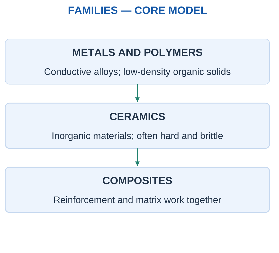
The syllabus groups materials into metals, polymers, ceramics and composites.
Each family contains many grades and forms. Family-level tendencies provide a starting point, while the actual supplied data determine a valid numerical comparison.

Avoid Absolute Rankings
Not every metal is denser than every composite.
Not every ceramic is an electrical insulator.
Not every polymer is flexible at its service temperature.
Material choice must match load, stiffness, mass, temperature, environment, cost and manufacturing.
A low purchase price can be outweighed by difficult joining, damage sensitivity or the need for a much larger section.
Worked Problem 1.61: Same-Volume Density Comparison
Problem: Candidate densities are 2700 and 7800 kg/m³. Each occupies 0.001 m³.
Step 1:
mA = 2700 × 0.001 = 2.7 kg
Step 2:
mB = 7800 × 0.001 = 7.8 kg
Step 3:
Reduction = (7.8 − 2.7)/7.8 × 100
Reduction = 65.3846%
Step 4: The lighter same-volume candidate still needs stiffness, strength, temperature and joining checks. A required geometry change can alter the final mass ranking.
Worked Problem 1.62: Another Density Comparison
Problem: Densities are 1600 and 2700 kg/m³. Both parts occupy 0.002 m³.
Step 1:
mA = 1600 × 0.002 = 3.2 kg
Step 2:
mB = 2700 × 0.002 = 5.4 kg
Step 3:
Reduction = (5.4 − 3.2)/5.4 × 100 = 40.7407%
Step 4: This comparison assumes equal volume. It does not establish equal stiffness, strength or service suitability.
21. Metals: Properties and Uses
Metals and alloys are used in structural members, shafts, fasteners, conductors and thermal paths.
Many combine useful strength with ductility and can be formed or machined.
Properties vary with alloy, processing and condition.
Ferrous materials have iron as their principal metal, including steels and cast irons.
Non-ferrous examples include aluminium and copper alloys.

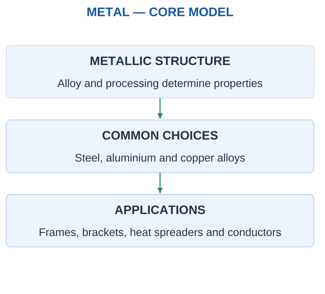
Aluminium alloys can be useful where low mass and suitable corrosion behaviour matter.
Steels can offer useful stiffness, strength and established joining routes.
Copper is familiar in electrical and thermal conduction duties.
These examples do not make one metal universally optimal.
Modulus and Strength
Two metal conditions can have similar modulus but different yield strengths.
Processing can change a strength limit without proportionally changing small-strain stiffness.
For equal volume:
m = ρV
For equal axial stiffness, geometry must also be included through AE/L.
Worked Problem 1.63: Two Metal Moduli at the Same Geometry
Problem: Two bars share F = 5000 N, L = 500 mm and A = 200 mm². EA = 200000 MPa and EB = 70000 MPa.
Step 1:
σA = σB = 5000/200 = 25 MPa
Step 2:
ΔLA = 5000 × 500/(200 × 200000) = 0.0625 mm
Step 3:
ΔLB = 5000 × 500/(200 × 70000) = 0.178571 mm
ΔLB/ΔLA = 2.85714
Step 4: The higher-modulus bar extends less. Strength and mass rankings require additional supplied values.
Metal Material Specimens


Density, modulus, strength and environment are different selection properties.
Equal geometry does not imply equal mass or deformation. The problem must identify the property governing the comparison.
22. Polymers: Housings, Insulation and Limits
Polymers contain long molecular structures and cover a wide range of behaviour.
Thermoplastics can soften and be reshaped under suitable processing conditions.
Thermosets form cross-linked networks and do not simply remelt into the same processable state.
Elastomers can show large recoverable deformation in their appropriate range.

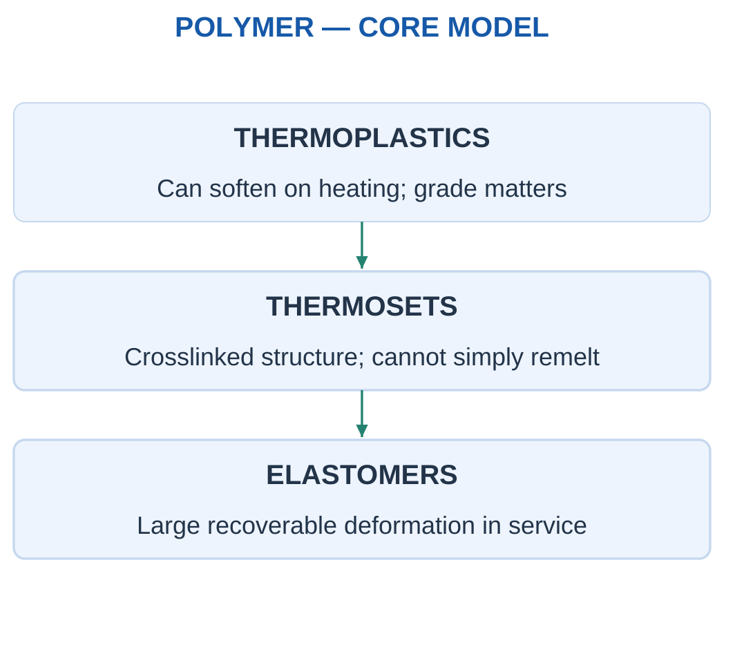
Many polymers offer low density, insulation and convenient moulding for covers, cable supports and enclosures.
Stiffness, strength, creep, temperature response, moisture sensitivity and fire performance depend on grade and conditions.
Creep
Creep is time-dependent deformation under sustained load.
A short-duration modulus may not predict long-term housing deformation.
A room-temperature property should not silently be applied to hot service.
Material Substitution
A flexible cable jacket and a stiff filled housing are both polymer-based but serve different functions.
A lower-density polymer does not automatically replace a metal frame at unchanged thickness while preserving stiffness and thermal behaviour.
Substitution may require geometry changes, inserts or a different joining route.
Worked Problem 1.64: Short-Duration and Long-Term Extension
Problem: A polymer member has F = 100 N, L = 100 mm, A = 50 mm² and short-duration E = 2000 MPa. A separately supplied long-term extension is 0.25 mm.
Step 1:
σ = 100/50 = 2 MPa
Step 2:
ΔLshort = 100 × 100/(50 × 2000) = 0.1 mm
Step 3:
Long-term/short-term ratio = 0.25/0.1 = 2.5
Step 4: The comparison shows why duration and temperature matter. A complete time-dependent prediction requires more data than one short-duration modulus.
Polymer Engineering Specimens

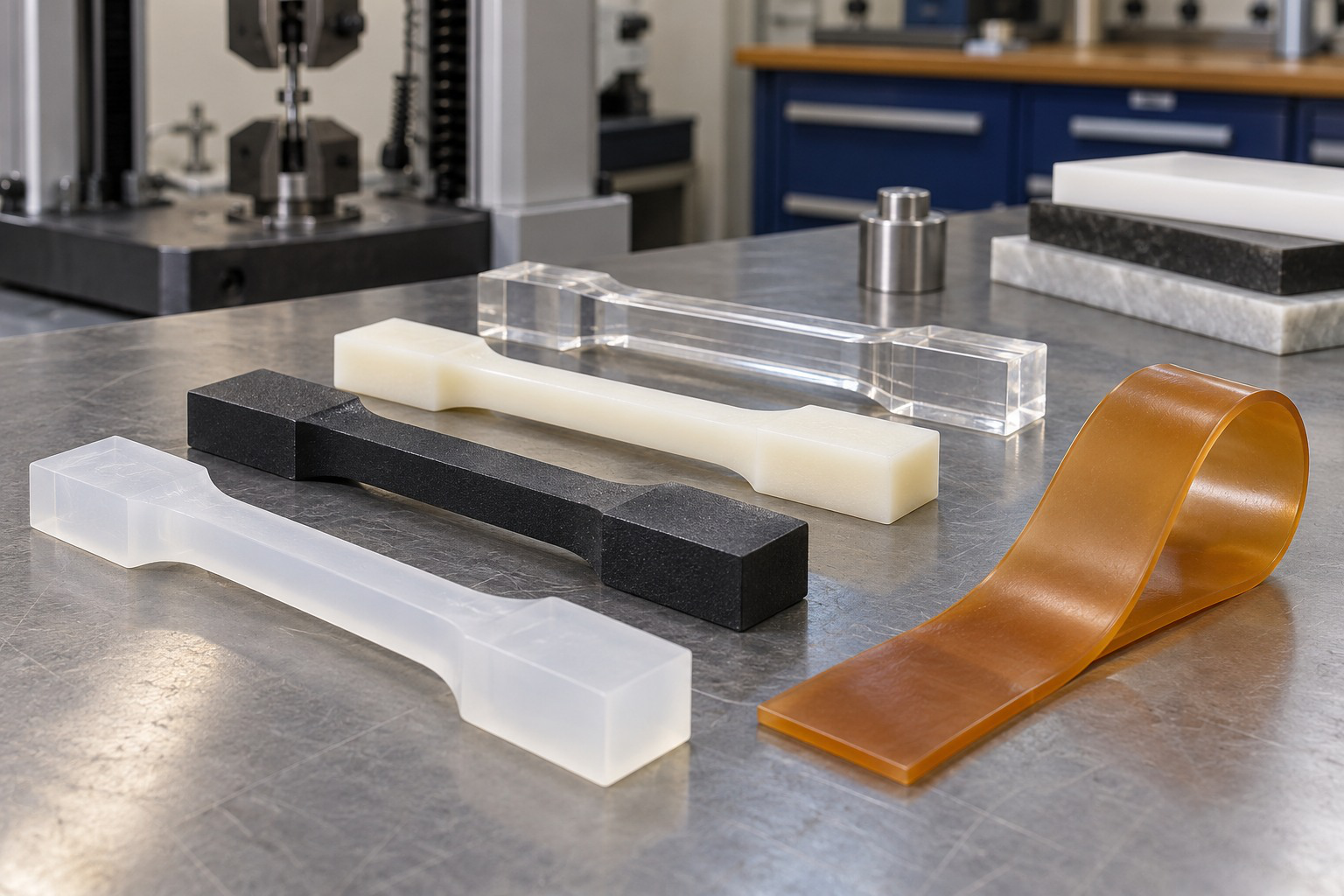
Low mass and processing advantages must be considered alongside time and temperature response.
Short-duration stiffness and long-term deformation are different observations.
23. Ceramics: Hardness, Insulation and Brittleness
Engineering ceramics include materials such as alumina and silicon carbide.
Glasses are another familiar inorganic class used in products.
Many ceramics offer hardness, wear resistance and stability at elevated temperature or in corrosive environments.

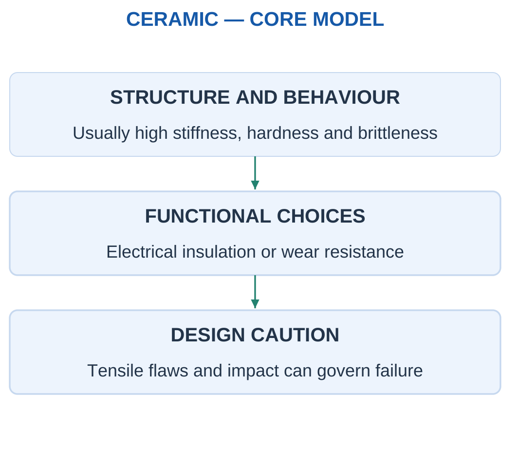
Many structural ceramics show limited plastic deformation before tensile fracture.
They can be sensitive to flaws, stress concentrations and impact.
High modulus does not automatically imply high toughness.
Some ceramics are insulators, while others have semiconducting, conducting, magnetic or other functional behaviour.
Loading Direction
Compression behaviour can differ greatly from tensile or impact behaviour.
Even a nominally compressive assembly can develop local tension or bending at a contact.
Ceramic selection should consider flaws, joints, thermal expansion compatibility, contact geometry and handling.
Ceramic Spacers

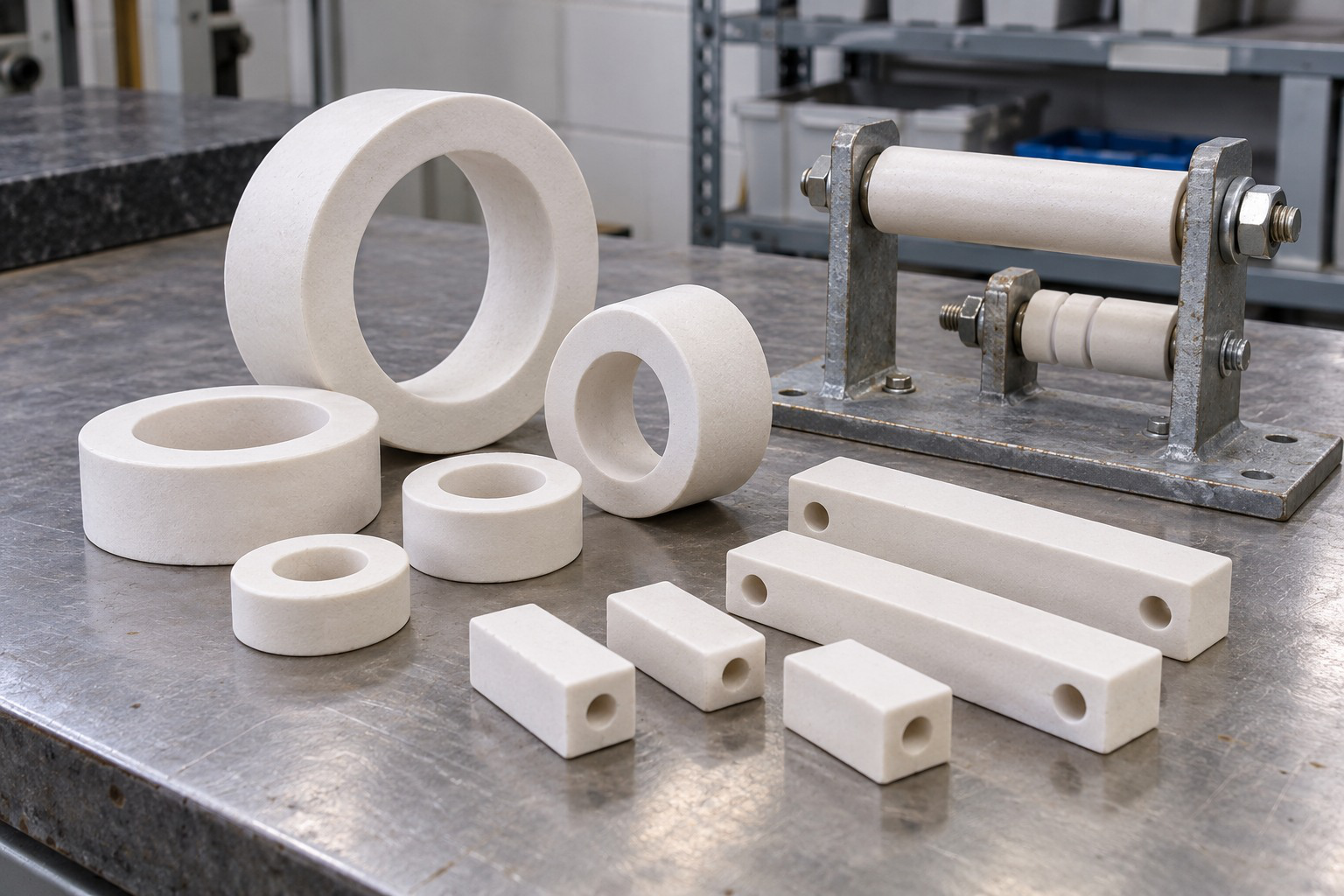
A ceramic can provide a useful thermal, electrical or compression function while brittleness remains important.
An average-stress check is narrower than a full failure assessment.
Worked Problem 1.65: Ceramic Spacer Compression
Problem: A short ceramic spacer carries centred compression of 8000 N over 200 mm². The supplied average-compression limit is 80 MPa.
Step 1:
σ = 8000/200 = 40 MPa
Step 2:
40 MPa ≤ 80 MPa
The stated average criterion passes.
Step 3:
Allowable/working ratio = 80/40 = 2
This is a numerical ratio under the supplied criterion, not an independently justified universal safety factor.
Step 4: Contact geometry, material condition, bending and other failure modes still require appropriate assessment.
24. Composites: Matrix, Reinforcement and Direction
A composite combines distinct constituents to obtain a useful property combination.
The matrix binds and supports the structure.
Reinforcement, such as fibres or particles, can add stiffness, strength or another useful function.
The interface transfers load between constituents.

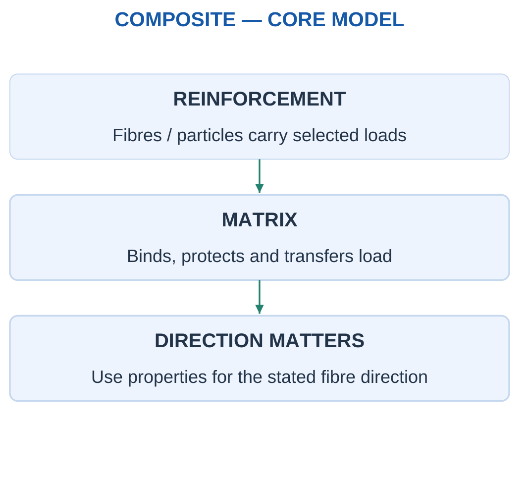
A fibre-reinforced polymer can offer low mass and useful stiffness in selected directions.
Different ply orientations can support different loading directions.
Performance depends on fibre, matrix, fraction, arrangement, bonding and damage condition.
Anisotropy
Anisotropy means properties vary with direction.
A high longitudinal modulus cannot automatically be used transverse to fibres or through a laminate thickness.
A robot-arm selection also requires torsion, joint, impact and manufacturing considerations.
A statement that a composite is “stronger than metal” is incomplete without property, direction and mass or geometry basis.
Worked Problem 1.66: Direction-Dependent Stiffness
Problem: A coupon has effective modulus 100000 MPa along reinforcement and 10000 MPa transversely. Use F = 2000 N, L = 300 mm and A = 100 mm².
Step 1:
σ = 2000/100 = 20 MPa
Step 2:
ΔLalong = 2000 × 300/(100 × 100000) = 0.06 mm
Step 3:
ΔLtransverse = 2000 × 300/(100 × 10000) = 0.6 mm
Extension ratio = 10
Step 4: Using the favourable along-fibre modulus in every direction would understate transverse extension.
Directional Composite Construction

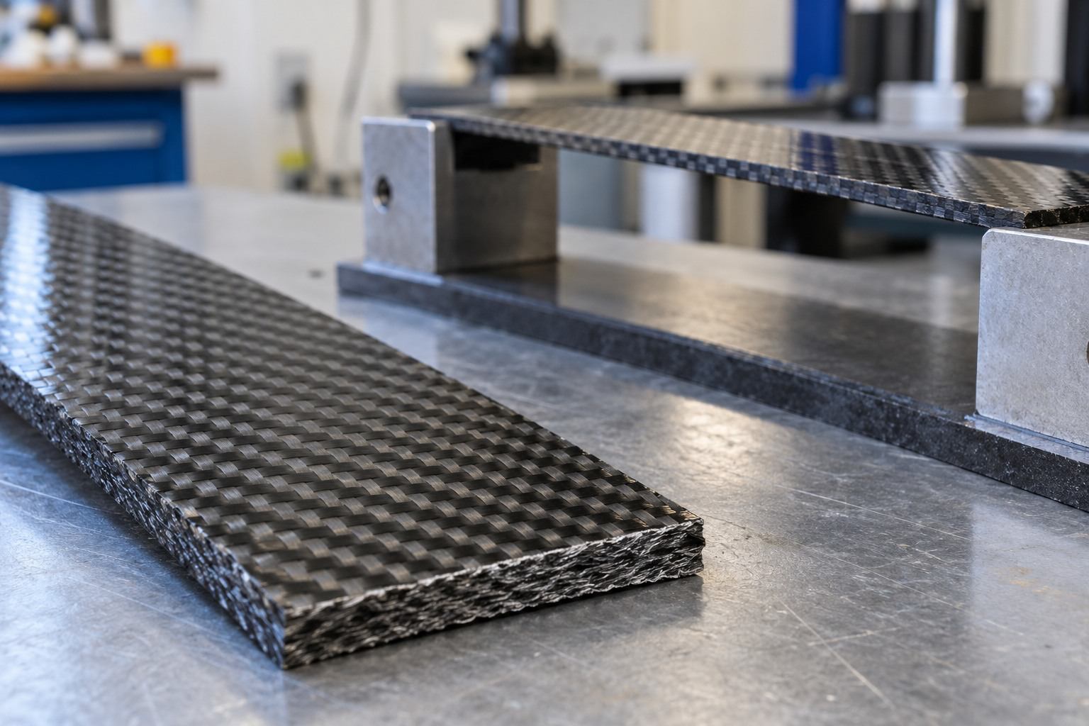
A supplied effective modulus belongs to its specified direction and construction.
A woven appearance is not a complete stiffness or strength specification.
25. A Clear Method for Basic Material Selection
Begin with function and constraints.
Separate requirements that must be met from objectives being improved.
A member may require a maximum extension and minimum strength while the objective is reduced mass or cost.

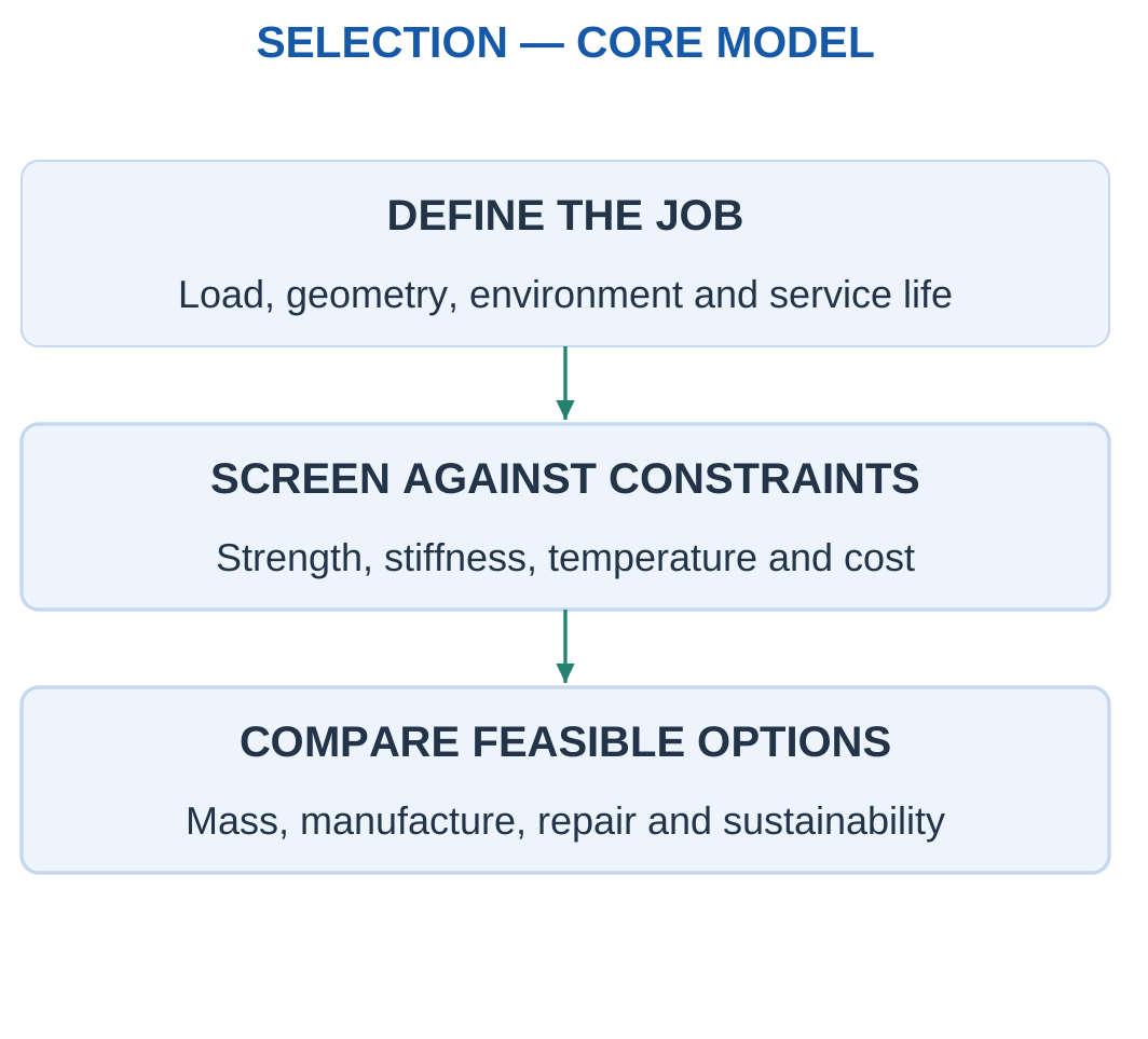
Selection Sequence
- Describe the load path and environment.
- Identify stiffness, strength and dimensional requirements.
- Check temperature, corrosion and electrical or thermal functions.
- Use density and property data with an explicit geometry.
- Consider processing, joining, repair and cost.
- State the reason and limits of the choice.
At identical geometry, stress depends on F/A, strain on E and mass on density.
If area changes to meet the same axial-stiffness target:
A = FL/(EΔLmax)
For fixed F, L and extension limit, mass scales with:
ρ/E
within this simplified axial comparison.
Comparison Basis
Same volume, same mass, same stiffness and same strength are different comparisons.
A material ranking can change when geometry is allowed to change.
Lightweight Vehicle Frame


Low density alone does not guarantee the lightest required component.
A stiffness requirement can force a larger section, changing the final mass.
Worked Problem 1.67: Equal Axial-Stiffness Requirement
Problem: A has density 1600 kg/m³ and E = 100000 MPa. B has density 2700 kg/m³ and E = 70000 MPa. Size both for F = 3000 N, L = 400 mm and ΔLmax = 0.08 mm.
Step 1:
AA = 3000 × 400/(100000 × 0.08) = 150 mm²
AB = 214.286 mm²
Step 2: Convert volume from mm³ to m³ using 10⁻⁹.
Step 3:
mA = 1600 × 150 × 400 × 10⁻⁹ = 0.096 kg
mB = 2700 × 214.286 × 400 × 10⁻⁹ = 0.231429 kg
Step 4: A is lighter under this stiffness requirement. Each candidate uses its own required area.
Worked Problem 1.68: Low Density but Low Modulus
Problem: A has density 1200 kg/m³ and E = 3000 MPa. B has density 2700 kg/m³ and E = 70000 MPa. Use F = 1000 N, L = 200 mm and ΔLmax = 0.2 mm.
Step 1:
AA = 1000 × 200/(3000 × 0.2) = 333.333 mm²
AB = 14.2857 mm²
Step 2: Use each required area to calculate volume.
Step 3:
mA = 1200 × 333.333 × 200 × 10⁻⁹ = 0.08 kg
mB = 2700 × 14.2857 × 200 × 10⁻⁹ = 0.00771429 kg
Step 4: B is lighter under this particular stiffness requirement despite its higher density.
Worked Problem 1.69: Screen Before Ranking
Problem: Candidate allowable stresses A/B/C are 40/80/120 MPa, moduli are 3/70/100 GPa and densities are 1200/2700/1600 kg/m³. The same-geometry member needs at least 60 MPa allowable stress and 50 GPa modulus.
Step 1: A fails both constraints.
Step 2: B and C pass both.
Step 3: Compare mass only among passing candidates. At equal volume, mass follows density.
Step 4: C has lower density than B and is the lower-mass feasible candidate under the supplied constraints.
Other service and manufacturing requirements were not supplied.
26. Laptop Frames and Server-Rack Load Paths
A laptop frame locates and protects components, supports hinges and fasteners and can contribute to heat flow.
A server rack transfers equipment load through shelves, rails, uprights and base supports.

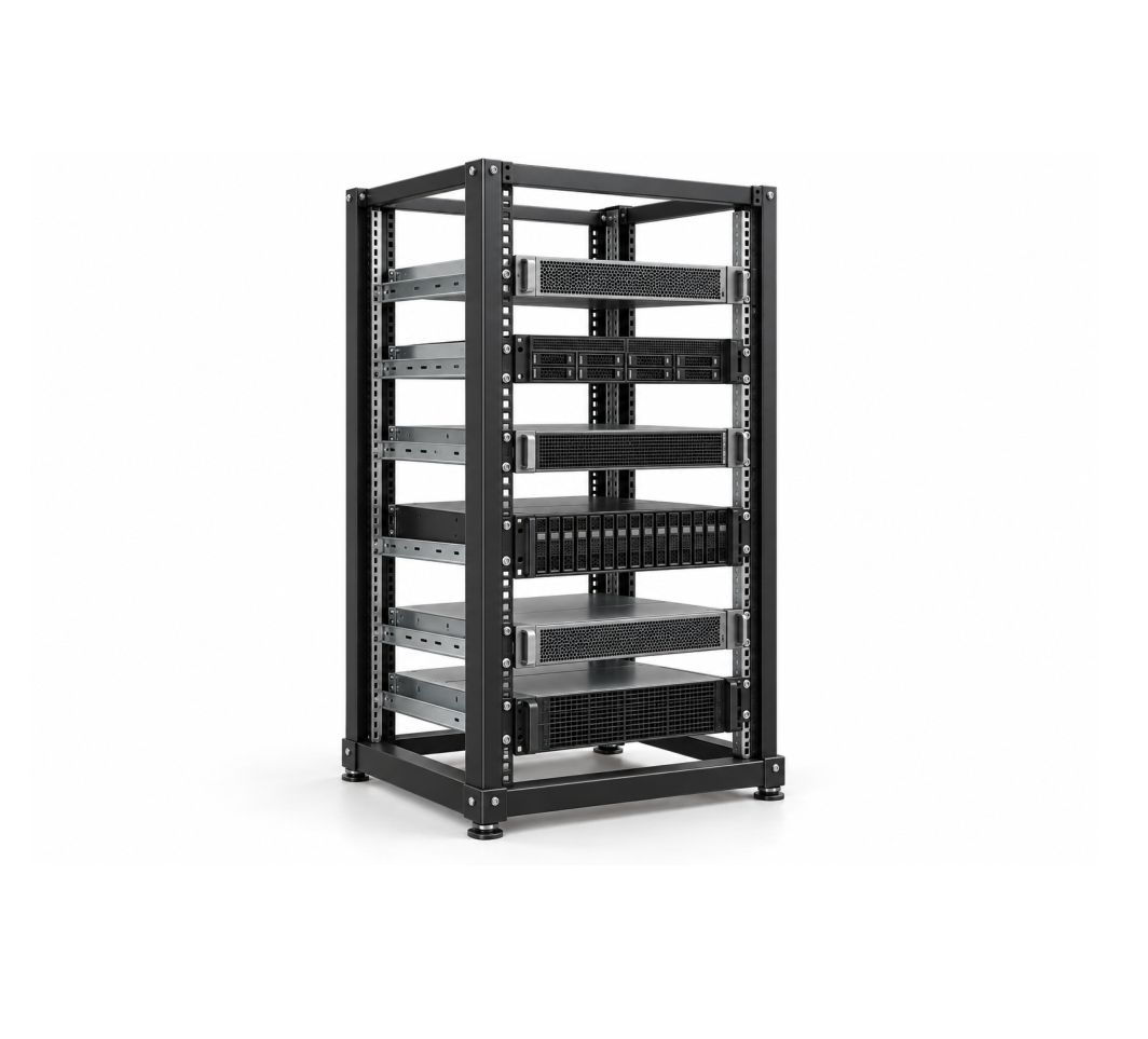


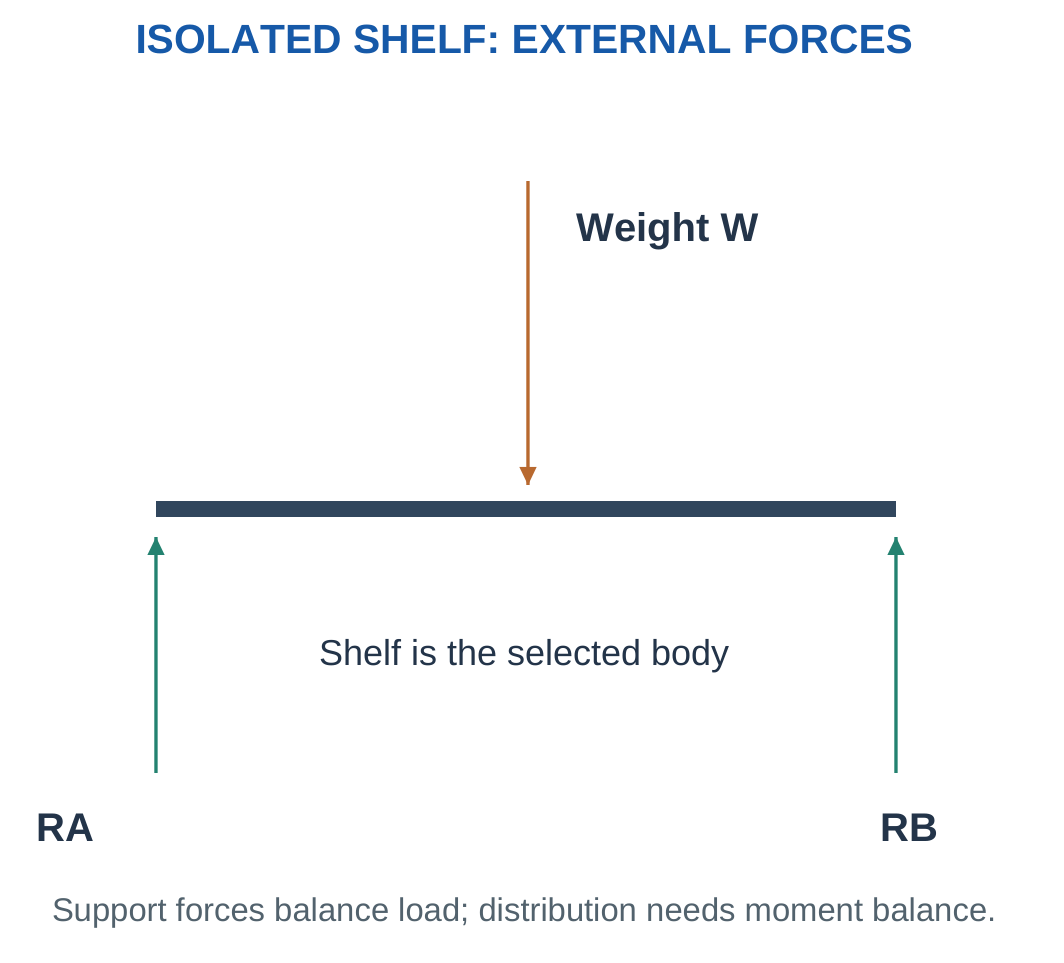
The model depends on the selected component.
A shelf can be a simply supported beam. A bracket can be a cantilever. A short upright can be an axial member in a separate model.
Do not apply all these models simultaneously to an undeclared body.
Stiffness and Alignment
A hinge force can create a moment because of its offset from the fastening region.
A frame can remain unbroken while moving enough to misalign a screen or connector.
Stiffness, geometry and joint behaviour therefore matter alongside strength.
Product Assumptions
Equipment weight, contact, joint behaviour and frame mass must be supplied or idealised.
The illustration does not establish manufacturer capacity.
A device can combine different families for structure, covers, insulation and thermal functions.
Worked Problem 1.70: Server-Shelf Reactions

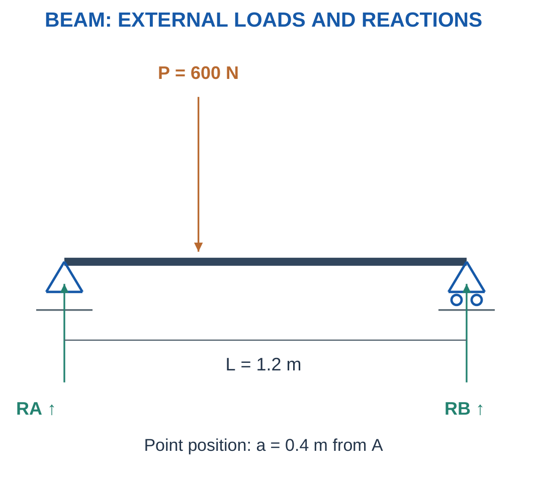
Step 1:
RA + RB = 600 N
Step 2:
RB × 1.2 = 600 × 0.4
Step 3:
RB = 200 N
RA = 400 N
Step 4:
RA × 1.2 = 600 × 0.8 = 480 N·m
The load lies nearer A, consistent with its larger reaction.
Worked Problem 1.71: Central Server Load
Problem: A 1.5 m shelf carries 900 N at 0.75 m from A.
Step 1:
RA + RB = 900 N
Step 2:
RB × 1.5 = 900 × 0.75
Step 3:
RB = 450 N
RA = 450 N
Step 4:
RA × 1.5 = 900 × 0.75 = 675 N·m
The central load gives equal reactions.
Worked Problem 1.72: Server Load Near B
Problem: A 1 m shelf carries 400 N at 0.7 m from A.
Step 1:
RA + RB = 400 N
Step 2:
RB × 1 = 400 × 0.7
Step 3:
RB = 280 N
RA = 120 N
Step 4:
RA × 1 = 400 × 0.3 = 120 N·m
The larger reaction occurs at the nearer right support.
Worked Problem 1.73: Laptop Bracket Average Stress
Problem: A simplified hinge bracket transfers 120 N centrally through 60 mm².
Step 1:
σ = 120/60 = 2 MPa
Step 2: A separate hinge moment would need geometry and an appropriate bending or joint model.
Step 3: The 2 MPa result is nominal average direct stress, not local screw-hole stress.
Step 4: Frame stiffness, joint movement, thermal paths and repeated opening loads can matter even when the average stress is small.
27. Tower-Antenna Supports: Weight and Lateral Force
An antenna support can carry downward weight and a lateral environmental resultant.
The lateral load creates a base moment when it acts above the support.
The introductory model uses the supplied resultant and height rather than predicting a complete wind load.

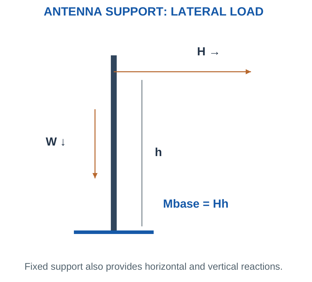
For lateral force H at height h:
Horizontal reaction magnitude = H
Base moment magnitude = Hh
A centred vertical weight through the reference point gives no moment about that point.
An eccentric weight would contribute an additional moment.
Guy Cables
Cable tension must be resolved using the angle convention.
A downward-running cable from an upper attachment can resist lateral loading while adding downward vertical loading.
Model Limits
Actual supports require environmental, dynamic, connection and stability assessment.
Keep horizontal and vertical loads as vectors. They should not be added as scalars before finding a resultant.
Worked Problem 1.74: Antenna Weight and Lateral Load
Problem: Weight is 100 N through the base reference. Lateral force is 200 N at height 2 m.
Step 1: Horizontal reaction is 200 N opposite the lateral load.
Step 2: Vertical reaction is 100 N upward.
Step 3:
M = 200 × 2 = 400 N·m
The centred weight has zero moment about the base reference.
Step 4:
R = √(200² + 100²) = 223.607 N
The support moment opposes the lateral turning effect.
Worked Problem 1.75: Larger Lateral Resultant
Problem: Weight is 150 N through the base reference. Lateral force is 350 N at height 1.5 m.
Step 1: Horizontal reaction is 350 N opposite the applied load.
Step 2: Vertical reaction is 150 N upward.
Step 3:
M = 350 × 1.5 = 525 N·m
Step 4:
R = √(350² + 150²) = 380.789 N
The force resultant and reaction moment are separate quantities.
Antenna Support and Bracket

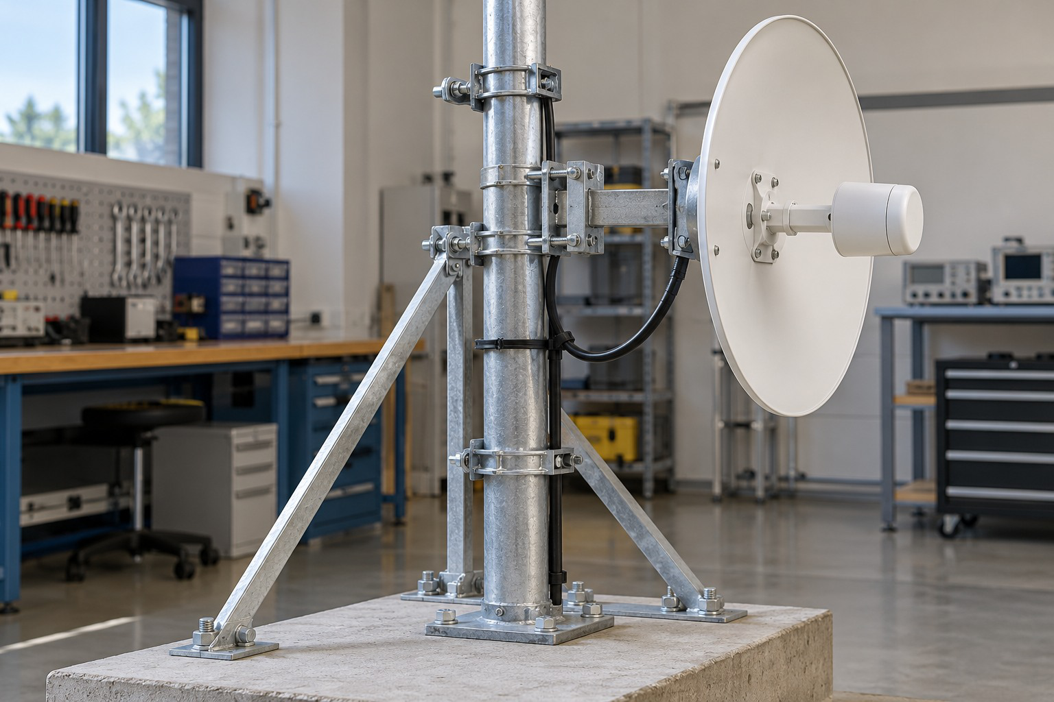
Centred weight and lateral force produce different effects.
A moment uses a perpendicular lever arm, rather than an arbitrary length visible in a photograph.
Worked Problem 1.76: Guy-Cable Components
Problem: A cable makes 40° to horizontal and must provide 300 N horizontal component.
Step 1:
H = T cos 40°
Step 2:
T = 300/cos 40° = 391.622 N
Step 3:
Vertical component = T sin 40° = 251.73 N
Step 4: If the cable runs down from the upper attachment to an anchor, its force on that attachment has a downward vertical component.
That component can add to vertical support loading.
28. Material Selection and Loads for a Robot Arm
A robot arm carries its structure, actuators and payload while positioning the end effector.
A payload away from a joint creates a moment. Link weight also creates a moment through its centre of gravity.
Neglecting self-weight must be an explicit simplification.

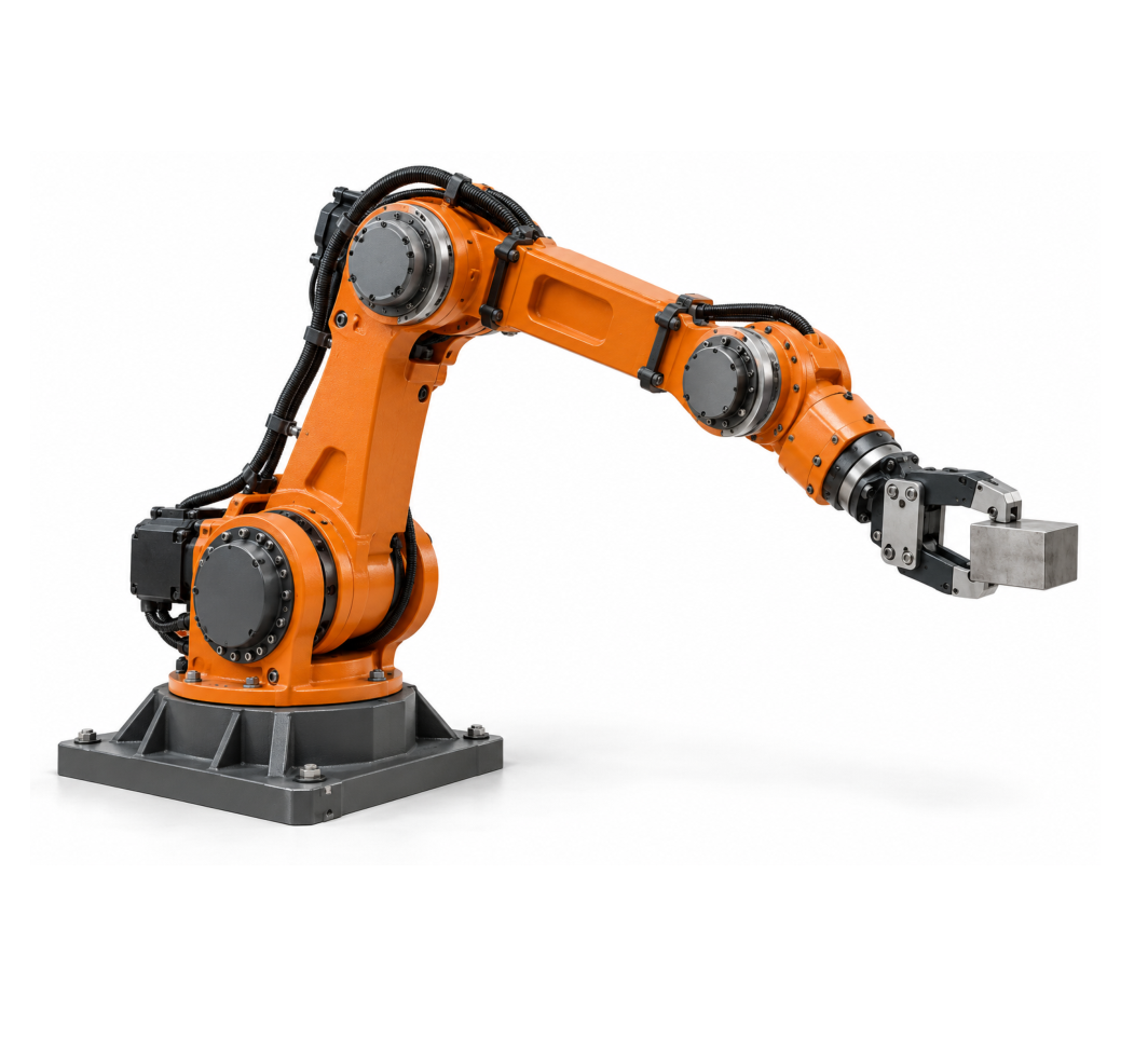

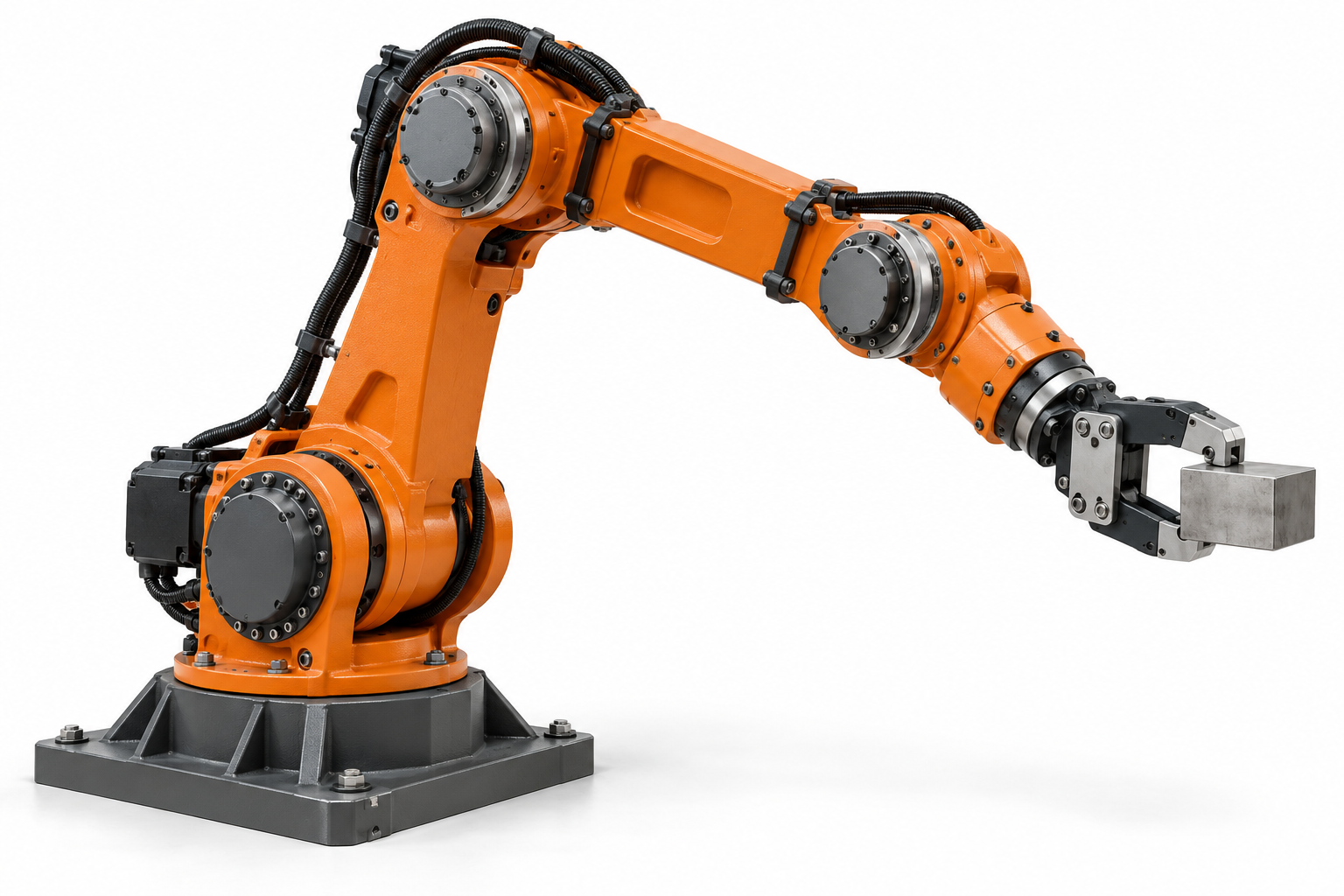

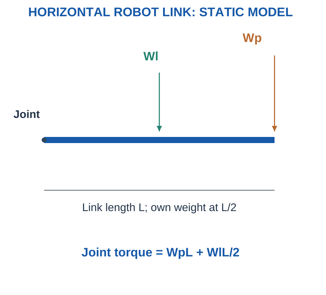
For a horizontal uniform link:
Mjoint = WpL + WlL/2
The payload acts at the tip and link weight acts at midspan.
Material and Positioning
Low density can reduce link weight, but stiffness must limit positioning error.
Composite direction, metal modulus, joint inserts, impact resistance and manufacturing can all influence selection.
Acceleration and changing configuration create loading beyond the static gravity model.
A gravity-moment calculation is not a complete actuator or payload rating.
Worked Problem 1.77: Horizontal Link Gravity Moment
Problem: Link length is 0.6 m, link mass 3 kg and tip payload mass 2 kg.
Step 1:
Wp = 2 × 9.81 = 19.62 N
Wl = 3 × 9.81 = 29.43 N
Step 2: Lever arms are 0.6 m and 0.3 m.
Step 3:
M = 19.62 × 0.6 + 29.43 × 0.3
M = 20.601 N·m
Step 4:
Total weight = 19.62 + 29.43 = 49.05 N
Dynamic, joint and operating limits need additional information.
Worked Problem 1.78: Longer Link
Problem: Length is 0.8 m, link mass 4 kg and tip payload 3 kg.
Step 1:
Wp = 29.43 N
Wl = 39.24 N
Step 2: Lever arms are 0.8 m and 0.4 m.
Step 3:
M = 29.43 × 0.8 + 39.24 × 0.4 = 39.24 N·m
Step 4:
Total weight = 68.67 N
The joint moment and total downward force are different loading requirements.
Worked Problem 1.79: Shorter Link
Problem: Length is 0.4 m, link mass 2 kg and payload mass 1.5 kg.
Step 1:
Wp = 14.715 N
Wl = 19.62 N
Step 2: Lever arms are 0.4 m and 0.2 m.
Step 3:
M = 14.715 × 0.4 + 19.62 × 0.2 = 9.81 N·m
Step 4:
Total weight = 34.335 N
The static result does not include acceleration or changing arm orientation.
Worked Problem 1.80: Axial-Stiffness Comparison for Link Material
Problem: An axial test uses F = 300 N, L = 800 mm and A = 200 mm². Candidate moduli are 70000 and 100000 MPa.
Step 1:
ΔLA = 300 × 800/(200 × 70000) = 0.0171429 mm
Step 2:
ΔLB = 300 × 800/(200 × 100000) = 0.012 mm
Step 3: The higher modulus reduces extension in this same-geometry axial test.
Step 4: Transverse robot-arm tip deflection requires beam geometry, support and joint behaviour and an appropriate bending model.
An axial extension must not be relabelled as transverse deflection.
29. EV Chassis: Structural Roles and Material Trade-Offs
An EV chassis locates major assemblies and transfers loads among wheels, body, occupants, battery supports and other components.
Actual vehicle loading is complex. Introductory exercises isolate a supplied part or simple load-sharing model.





Metals can provide established forming and joining routes and useful ductility.
Polymers can serve covers and insulation. Composites can provide targeted lightweight stiffness. Ceramics can serve selected thermal and electrical roles.
The product is a material system rather than one family used for every function.
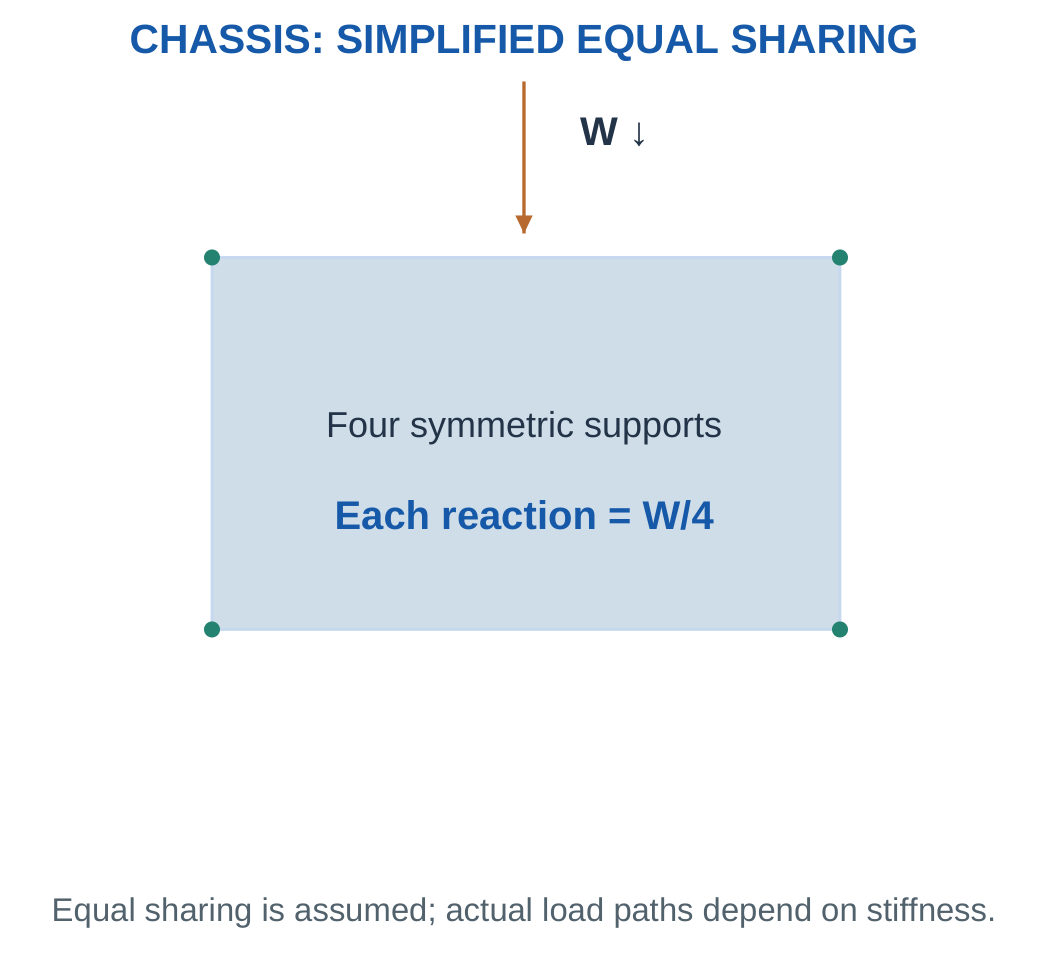
Support Sharing
Real vehicle corner loads are not always one-quarter of total weight.
Distribution depends on centre of gravity, geometry, stiffness and operating condition.
Crashworthiness, fatigue, battery enclosure requirements and complete vehicle design lie beyond the elementary direct-stress model.
Worked Problem 1.81: Four Equal Supports
Problem: A simplified platform carries 400 kg equally on four supports. Each resisting area is 500 mm².
Step 1:
W = 400 × 9.81 = 3924 N
Step 2:
Fsupport = 3924/4 = 981 N
Step 3:
σ = 981/500 = 1.962 MPa
Step 4: Equal sharing follows the supplied model. It is not a universal rule for every EV operating condition.
Worked Problem 1.82: Three Equal Supports
Problem: A simplified platform carries 240 kg equally on three supports. Each resisting area is 300 mm².
Step 1:
W = 240 × 9.81 = 2354.4 N
Step 2:
Fsupport = 2354.4/3 = 784.8 N
Step 3:
σ = 784.8/300 = 2.616 MPa
Step 4: A different support geometry or stiffness distribution could invalidate equal sharing.
Worked Problem 1.83: Same-Volume Chassis-Member Mass
Problem: Volume is 0.003 m³. Candidate densities are 7800 and 2700 kg/m³.
Step 1:
m1 = 7800 × 0.003 = 23.4 kg
Step 2:
m2 = 2700 × 0.003 = 8.1 kg
Step 3:
Saving = 23.4 − 8.1 = 15.3 kg
Percentage saving = 65.3846%
Step 4: The lighter same-volume member still needs stiffness, strength, joining and service checks.
A required geometry change can alter the final saving.
30. Formula Sheet and Examination Approach
| Quantity | Relation |
|---|---|
| Weight | W = mg |
| Horizontal component | Fx = F cos θ |
| Vertical component | Fy = F sin θ |
| Resultant magnitude | R = √(Rx² + Ry²) |
| Force moment | M = Fdperp |
| Component moment | M = xFy − yFx |
| Planar static equilibrium | ΣFx = 0, ΣFy = 0, ΣM = 0 |
| Average normal stress | σ = F/A |
| Average simple shear | τ = V/Ashear |
| Engineering strain | ε = ΔL/L0 |
| Linear elasticity | σ = Eε |
| Uniform axial extension | ΔL = FL/(AE) |
| Axial stiffness | k = AE/L |
| UDL resultant | W = wl |
| UDL resultant location | Loaded-segment midpoint |
| Simply supported point load | RB = Wa/L, RA = W − RB |
| Cantilever tip-load moment | WL |
| Full-length cantilever UDL moment | wL²/2 |
| Mass from volume | m = ρV |
| Minimum stress-based area | F/σallow |
| Minimum extension-based area | FL/(EΔLmax) |
Method Across the Unit
Choose the body, draw loads and reactions, state assumptions, convert units and write equilibrium or the relevant constitutive relation.
Substitute with units and interpret the result.
For material selection, establish constraints before ranking mass or cost.
Quick Checks
- N/mm² equals MPa.
- Strain is dimensionless.
- UDL intensity needs a loaded length to become force.
- Zero net force does not imply zero moment.
- A large modulus does not prove high strength or toughness.
- Equal support count does not prove equal load share.
- A stress result belongs to a specified section and loading model.
- A passed introductory criterion does not establish a complete product rating.
31. Short Questions with Clear Answers
1. How Do Mass and Weight Differ?
Mass is measured in kilograms.
Weight is gravitational force:
W = mg
It is measured in newtons.
A load already supplied in N does not require another multiplication by g.
2. Can a Force Deform a Body Without Moving It Overall?
Yes.
Supports can balance external loads while internal stress and deformation develop.
Static equilibrium means the force and moment balances are satisfied. It does not mean the body is unstressed or undeformed.
3. Why Does a Free-Body Diagram Isolate One Body?
Only external actions on that body belong in its equilibrium equations.
Mixing forces from different bodies can double-count an interaction or cancel a force incorrectly.
The selected body determines which contact forces become external reactions.
4. What Is a Moment Arm?
It is the perpendicular distance from the reference point to the force’s line of action.
It is not automatically the complete distance to the application point.
The moment equation must use the perpendicular geometry.
5. Can Zero Net Force Coexist with a Turning Tendency?
Yes.
A couple contains equal opposite forces with separated lines of action.
The resultant force is zero, but the couple moment is nonzero.
Both force and moment equations are needed for planar equilibrium.
6. Why Is Stress Different from Force?
Stress describes force intensity per resisting area.
The same axial force produces a larger average stress when the section is smaller.
Force is measured in N; stress is measured in Pa, MPa or another force-per-area unit.
7. Does Strain Have a Unit?
Engineering strain is a ratio of consistently expressed lengths and is dimensionless.
It can be written as a decimal, percentage or microstrain.
These forms are alternative representations of the same ratio.
8. Does a Larger E Mean a Larger Failure Load?
Not by itself.
E describes linear-elastic stiffness.
Failure load also depends on strength, geometry, loading mode, defects and other limits.
A stiffness ranking and strength ranking can differ.
9. How Do Elasticity and Ductility Differ?
Elasticity concerns recovery after unloading.
Ductility concerns plastic deformation before fracture.
Large strain alone does not identify whether the deformation was recoverable or permanent.
10. Where Does a Full-Span UDL Resultant Act?
At the midpoint of the uniformly loaded span.
For a partial UDL, use the loaded segment’s midpoint.
It is not automatically the centre of the entire beam.
11. Do Equal Beam Supports Always Carry Equal Loads?
No.
Equal reactions follow from the stated symmetric loading and support conditions.
An off-centre load usually produces unequal reactions, with the nearer support carrying more.
12. Why Can a Ceramic Be Stiff but Brittle?
Its modulus can be high while plastic deformation before fracture is small.
Stiffness and fracture-energy behaviour are different properties.
High stiffness does not automatically provide high toughness.
13. Why Is Fibre Direction Important in a Composite?
Composite properties can vary strongly with direction.
An along-fibre modulus or strength cannot automatically be assigned transversely or through the laminate thickness.
The property must match the actual loading direction.
14. Is the Lightest Same-Volume Material Always Best for an Arm?
No.
It may fail stiffness, strength, temperature, joining or damage constraints.
Selection screens required constraints before ranking mass.
The required geometry can change the final mass comparison.
15. Does a Passed Average-Stress Check Certify a Product?
No.
It verifies only the stated average direct-stress criterion.
Local stress, bending, stability, fatigue, joints and actual service conditions may still govern.
32. Complete Examination Answers
1. Explain Force Effects and Static Equilibrium
A force has magnitude, direction and line of action.
It can produce translation, rotation or deformation depending on the supports and geometry.
Resolve non-collinear loads into horizontal and vertical components before adding them.
The planar resultant follows from ΣFx and ΣFy, but zero resultant force alone does not establish zero moment.
For static equilibrium:
ΣFx = 0
ΣFy = 0
ΣM = 0
A couple demonstrates that zero force resultant can coexist with a finite turning effect.
Begin with an isolated free-body diagram showing external loads, allowed support reactions and dimensions.
Keep action and reaction on their appropriate bodies. Drawing both on one isolated body can cancel an interaction incorrectly.
2. Explain Stress, Strain and the Linear Extension Relation
Average direct stress is:
σ = F/A
for a centrally loaded section under the stated uniform model.
Engineering strain is:
ε = ΔL/L0
It is dimensionless.
Within a linear-elastic uniaxial range:
σ = Eε
Substitution gives:
ΔL = FL/(AE)
E is a material modulus, while member stiffness AE/L also depends on geometry.
Use consistent units, such as N, mm², mm and MPa.
The relation does not establish local hole stress, buckling resistance or arbitrary plastic deformation.
Compression can be represented through a consistent sign convention or an explicitly identified positive magnitude.
3. Distinguish Important Mechanical Properties
Stiffness describes resistance to elastic strain.
Strength describes a specified stress limit.
Hardness describes resistance to local indentation or scratching under its test.
Toughness concerns energy absorbed before fracture.
Ductility describes plastic deformation capacity, while brittleness indicates relatively little plastic deformation before fracture.
Elasticity concerns recovery after unloading.
A stiff ceramic can be brittle. A polymer can undergo large recoverable strain while having a lower modulus than a metal.
Density affects mass for a given volume.
Values vary with grade, direction, processing, temperature and test conditions.
A valid selection identifies the relevant property instead of treating one material family as automatically strongest, toughest and lightest.
4. Explain Point Loads and UDLs on Beams
A point load represents a concentrated force at a stated location.
A UDL has constant force per length w over loaded length l.
Its total force is:
W = wl
and its equivalent resultant acts at the loaded segment’s midpoint.
For simply supported beams, a moment equation determines one reaction and vertical equilibrium gives the other.
A central point load W gives W/2 at each support under symmetric conditions.
An off-centre point load gives unequal reactions.
A full-span symmetric UDL gives wL/2 at each support.
Replacing a UDL by its resultant preserves external force and moment, but not every local internal-force or deformation distribution.
5. Compare Metals, Polymers, Ceramics and Composites
Metals commonly offer useful structural strength, ductility and conductivity, with alloy-dependent density and corrosion behaviour.
Polymers often offer low density, insulation and convenient shaping. Temperature and creep can govern their performance.
Ceramics can offer hardness, wear resistance, temperature stability and selected insulating functions. Brittleness and flaw sensitivity require attention.
Composites combine matrix and reinforcement to provide a useful property set. Fibre arrangement can create strong directional dependence.
These are tendencies rather than universal rules.
Use actual data with load, geometry, environment and joining requirements.
A product can combine metal frames, polymer covers, ceramic insulators and composite panels because the functions differ.
6. Explain a Laptop or Server-Rack Load-Path Application
Select the component before choosing the model.
A server shelf can be represented as a simply supported beam carrying equipment point loads or a supplied UDL.
Shelf reactions transfer load to uprights and base supports.
A laptop hinge can apply an offset force and moment to its fastening region.
Stiffness matters because excessive movement can misalign a display, connector or equipment rail even if no part breaks.
Material choice must consider mass, strength, modulus, heat flow, durability and manufacturing.
Calculate from supplied assumptions rather than inferring capacity from an illustration.
Equal sharing requires symmetry or an explicit model. Real joints and local stresses need additional checks.
7. Explain Robot-Arm Material and Loading Considerations
A horizontal link carries payload and self-weight.
The payload at the tip has lever arm L. Uniform-link weight acts at L/2.
The simplified gravity moment is:
M = WpL + WlL/2
Moving the same force nearer the joint reduces moment.
Low density can reduce self-weight demand, but modulus, geometry and joint stiffness must maintain positioning accuracy.
Composite direction and damage, metal stiffness and ductility, joining and manufacture all matter.
Acceleration and changing configuration introduce additional loads beyond the static model.
A gravity-moment calculation therefore does not establish a complete actuator rating or certified payload.
8. Explain a Basic Material-Selection Procedure
Define function, loads, supports, temperature, environment and interfaces.
Separate constraints from objectives.
Allowable stress and maximum extension are constraints. Low mass or cost can be objectives.
For a uniform axial member:
A ≥ F/σallow
and:
A ≥ FL/(EΔLmax)
Use the larger area requirement.
Screen candidates against all constraints before ranking those that remain.
Calculate mass from density and the actual required volume rather than assuming equal volume automatically.
Consider manufacturing, joining, repair, corrosion and directional properties.
State why the candidate satisfies the supplied model and identify the limits of the comparison.
9. Solve and Interpret a Combined Shelf Load
Question: A 2 m simply supported shelf carries a full-span 100 N/m UDL and a 120 N point load 0.5 m from A. Find the reactions and explain assumptions.
Step 1: Replace the UDL with its resultant.
U = 100 × 2 = 200 N
It acts 1 m from A.
Step 2: Take moments about A.
RB × 2 − 200 × 1 − 120 × 0.5 = 0
RB = 130 N upward
Step 3: Apply vertical equilibrium.
RA + 130 − 200 − 120 = 0
RA = 190 N upward
Step 4: Check force and moment balances.
190 + 130 = 320 N
190 × 2 = 200 × 1 + 120 × 1.5 = 380 N·m
The greater left reaction agrees with the extra point load being nearer A.
The model uses an ideal pin and horizontal frictionless roller, static loading and the stated positions.
Self-weight is omitted unless already included in the UDL.
The reactions establish external equilibrium, not maximum bending stress, deflection or rated shelf capacity.
33. Integrated Revision: From Load to Material Choice
Start with the Body
The selected body defines the external forces.
A whole shelf diagram includes equipment loads and support reactions. An imaginary section through a member introduces internal forces for that cut.
A support and shelf exert equal opposite forces on different bodies. Both should not be placed on the same isolated shelf diagram.
This body-selection step prevents incorrect cancellations and double counting before algebra begins.
Preserve Force and Position
A load system is not fully described by its total force alone.
A point load’s location determines its moment. A UDL’s loaded length determines total force, and its segment midpoint determines the resultant location.
Two arrangements can have the same total downward force but different reactions or support moments.
Keep each load’s position until the moment equation has been written.
Separate Equilibrium from Capacity
Equilibrium determines reactions under a supplied loading model.
Stress and deformation calculations then describe the selected component’s response under additional assumptions.
A reaction calculation does not identify maximum safe load.
Similarly, a low average stress does not establish that deflection, buckling, joints or fatigue are acceptable.
These questions need their own data and appropriate models.
Separate Material Properties
Modulus describes elastic stiffness. Strength describes a limiting stress. Density affects mass.
A candidate can be stiff but have a lower strength limit, or low-density but require a much larger section.
A sound comparison names the property and geometric basis before ranking candidates.
Keep Geometry in the Comparison
For equal force and area, average axial stress is the same regardless of modulus.
For equal stress, strain varies inversely with E.
For equal volume, mass varies with density.
For the same axial-stiffness requirement, the required area changes with modulus, so density alone no longer determines final mass.
These are different comparisons and can produce different rankings.
34. Common Numerical Errors and Corrections
Multiplying an Existing Force by g
A value in newtons is already a force.
Use mg only when converting a supplied mass into weight.
Multiplying an existing force by g introduces an incorrect additional factor and incompatible interpretation.
Adding Perpendicular Forces as Scalars
A horizontal 60 N force and vertical 80 N force give a 100 N resultant, not 140 N.
Resolve and combine components.
The direction must also be determined from their signs.
Using the Wrong Moment Arm
Moment uses perpendicular distance to the force line.
For component methods, use:
M = xFy − yFx
A diagonal distance to the application point is not automatically the correct lever arm.
Checking Only Vertical Equilibrium
RA + RB = W gives one equation for two unknown reactions.
A moment equation establishes how the load is distributed.
Equal supports alone do not justify equal reactions under asymmetric loading.
Using Outer Area for a Hollow Member
The void does not resist direct axial load.
Subtract inner area from outer area.
Using the full outer circle understates average stress.
Mixing Millimetres and Metres in Strain
Strain requires the same length unit in numerator and denominator.
Convert before dividing.
A dimensionless result can still be numerically wrong if the unit conversion was omitted.
Mixing MPa and Numerical GPa Values
Convert E to the same stress unit as σ.
For example:
70 GPa = 70000 MPa
The numerical value 70 cannot be used with σ in MPa without conversion.
Treating Modulus as Strength
A larger E reduces elastic strain at a given stress.
It does not by itself establish a larger failure load.
Use the supplied strength criterion separately.
Treating UDL Intensity as Total Force
Multiply intensity by loaded length.
Then place the resultant at the loaded segment’s midpoint.
Do not use the whole-beam centre for every partial UDL.
Ranking Density Before Screening Constraints
The lowest-density candidate can fail stiffness or strength requirements.
Screen first, then compare the objective among feasible candidates.
When geometry changes, calculate the resulting volume rather than retaining a same-volume assumption.
Relabelling Axial Extension as Bending Deflection
The formula FL/(AE) describes a uniform central axial model.
Transverse tip deflection needs the appropriate beam and section model.
The two deformations are physically different even though both are measured in millimetres.
35. Application Connections
Laptop Frames and Material Systems
A laptop frame can contribute to positioning, protection and thermal transfer.
A metal frame, polymer cover and insulating component can coexist because each serves a different role.
The material decision must follow the component’s function, load path and environment.
A single family-level adjective cannot establish the best choice for every part.
Server Racks and Support Conditions
A shelf’s reactions depend on loading and support positions.
The rack uprights then receive those reactions as loads in a larger selected-body model.
Changing the selected body changes which forces are external.
This is why a shelf calculation and a full-rack calculation should not be combined without declaring the boundary.
Antenna Supports and Direction
Weight and lateral force act in different directions.
The centred weight contributes vertical force, while the lateral force at height produces a moment.
A guy cable can resist horizontal loading while adding a vertical component.
Resolving directions makes these contributions visible before they are combined.
Robot Arms and Self-Weight
Reducing link mass can reduce gravity moment.
However, a flexible link can degrade positioning even if its strength is adequate.
Material, section shape and joints must therefore be considered together.
Static calculations explain a basic requirement but do not include every moving-operation effect.
EV Platforms and Equal Sharing
An equal-sharing example is useful for practising mass-to-weight conversion and direct stress.
Actual distribution can vary with centre of gravity, geometry, stiffness and operating condition.
The simplified result should be retained with its stated assumptions rather than treated as a universal vehicle rule.