
University: Dr. A.P.J. Abdul Kalam Technical University (AKTU)
Programme: B.Tech First Year, Semester I & II
Course Codes: AME101A / AME201A
Branches: Common to All
Unit: V — Mechatronics, Robotics and Emerging Mechanical Systems
Introduction to Mechatronics, Robotics and Emerging Mechanical Systems
Modern mechanical systems increasingly combine physical mechanisms with electronics, sensors, computation and controlled actuation. A machine must do more than contain these components. The components must exchange information and energy in a way that performs the required task.
A printer axis, robotic arm or drone illustrates this integration. Its mechanism carries the load, actuators create motion, sensors describe relevant physical conditions and a controller determines an action. A driver connects the controller’s command with the actuator’s power supply.
This unit develops these relationships through DC motors, stepper motors, servo systems, hydraulic and pneumatic actuators, robot arrangements, drone subsystems and connected manufacturing.
The central questions are what moves, what supplies the energy, what is measured and how that information affects the next action.
Unit Coverage
- Mechatronics and system integration.
- Information flow and energy flow.
- Sensors, calibration and signal scaling.
- Open-loop and closed-loop control.
- Requirement-based actuator selection.
- DC motors, torque, speed and losses.
- Drivers, commands and motion mechanisms.
- Stepper motors and nominal command increments.
- Servo systems and encoders.
- Hydraulic and pneumatic actuation.
- Robot joints, links and degrees of freedom.
- Cartesian, SCARA and articulated robots.
- End effectors, workspace and cycle time.
- Drone airframe, propulsion and flight controller.
- Static hover calculations.
- Industry 4.0 and connected manufacturing.
- Condition monitoring and digital twins.
- Formula revision and examination answers.
Important Terms
| Term | Meaning |
|---|---|
| Sensor | Measures a physical quantity |
| Actuator | Produces physical force, torque or motion |
| Controller | Determines an action from the task and available information |
| Driver | Interfaces a command with actuator power |
| Feedback | Information returned about the represented process |
| Reference | Desired value of a controlled quantity |
| Error | Difference defined between reference and measurement |
| Resolution | Represented increment under a stated measurement or command model |
| Accuracy | Closeness to the relevant reference or actual value |
| Repeatability | Closeness of repeated results under stated conditions |
| End effector | Tool or handling device at a robot’s working end |
| Digital twin | Purposeful digital representation connected with a physical system |
Working Conventions
Reduction is defined as input speed divided by output speed. Encoder counts include decoding only when explicitly stated. Stepper calculations describe nominal followed commands unless measured motion is supplied.
Cylinder areas, pressure references and flow conditions must be named. All numerical limits, material properties and efficiencies in the problems are supplied educational values.
1. Mechatronics: Integration Rather Than a Parts List
Mechatronics combines mechanical systems, electronics, sensing, actuation, computation and control to perform a useful task.
Integration means that the components are selected and arranged to work together. A motor alone is an actuator. A complete positioning axis also needs a mechanism, guidance, power interface, command source and appropriate measurements.

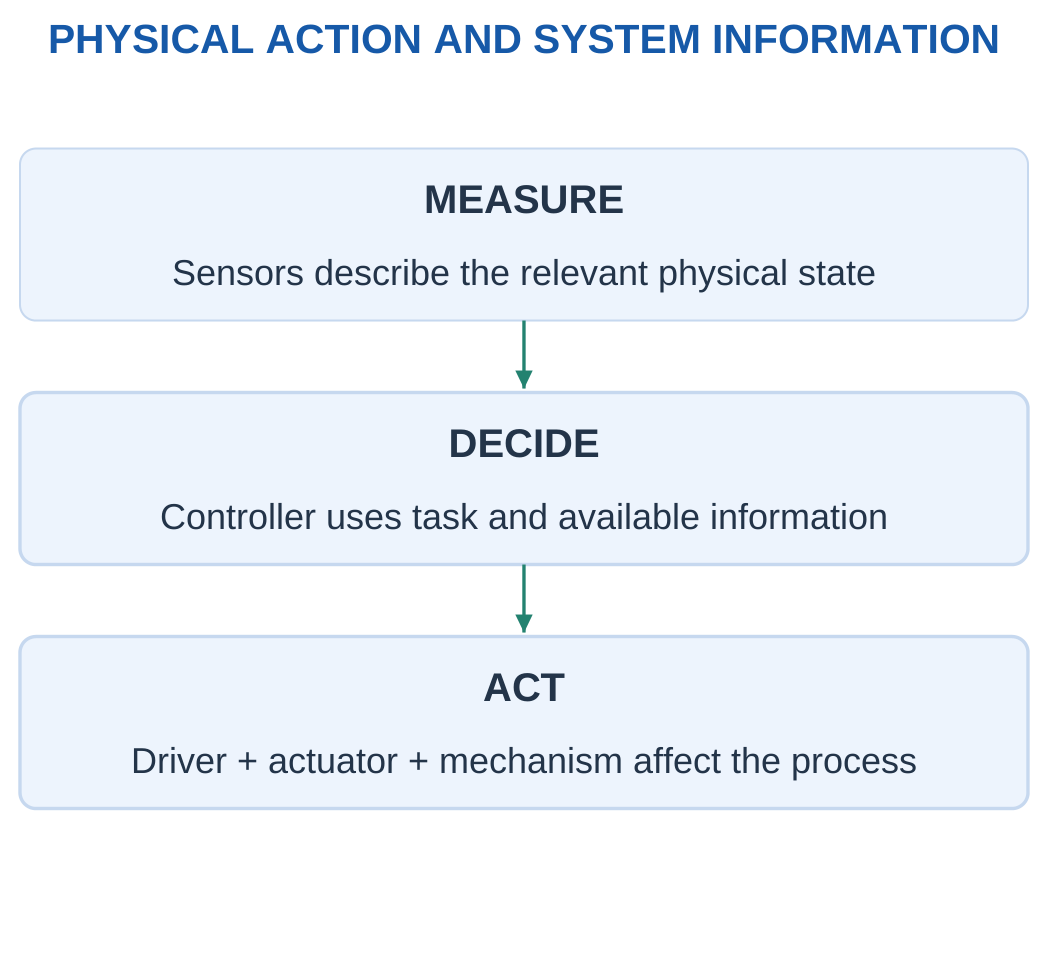
A printer axis provides a useful example. A controller issues commands. A driver supplies controlled electrical power to the motor. A screw or belt converts rotation into carriage travel. A guide constrains the carriage.
A sensor or home switch supplies information according to the chosen arrangement. A home switch identifies a reference event; it does not necessarily measure every intermediate carriage position.
Reading a Mechatronic System
Ask four questions:
- What physical quantity must be controlled?
- Which actuator and mechanism produce the action?
- What information is available about the process?
- How does the controller use commands and measurements?
A useful explanation follows the connections. Listing a sensor, motor and controller without explaining their interactions does not show how the task is completed.
Energy Balance
For a supplied steady system:
Useful output power = Efficiency × Input power
Represented loss rate = Input power − Useful output power
Useful output energy = Useful output power × Time
These relations require a consistent system boundary. A motor-only efficiency should not automatically be treated as the efficiency of an entire mechanism and driver.
Worked Problem 5.1: Actuator-System Energy Balance
Problem: A steady actuator system receives 120 W and has useful mechanical efficiency 0.75. It operates for 40 s. Find output power, loss rate and useful output energy.
Solution:
Output power = 0.75 × 120 = 90 W
Loss rate = 120 − 90 = 30 W
Useful energy = 90 × 40 = 3600 J
The input energy is 4800 J. The remaining 1200 J belongs to the represented loss terms under the steady model.
Answer: Useful output is 90 W, loss rate is 30 W, and useful output energy is 3600 J.
Worked Problem 5.2: Another System Boundary
Problem: Input power is 200 W, useful efficiency is 0.8 and operating time is 30 s.
Solution:
Output power = 0.8 × 200 = 160 W
Loss rate = 200 − 160 = 40 W
Useful energy = 160 × 30 = 4800 J
Answer: Output is 160 W, loss is 40 W, and useful energy is 4800 J.
The calculation describes the complete supplied boundary. It does not separately identify the driver, motor and transmission losses unless those terms are given.
2. Information Flow and Energy Flow
A signal path carries information such as a command, measurement or status value. A power path supplies the energy required for physical action.
A small command signal can control a much larger actuator power through a suitable driver. The command signal does not itself supply all the mechanical output energy.

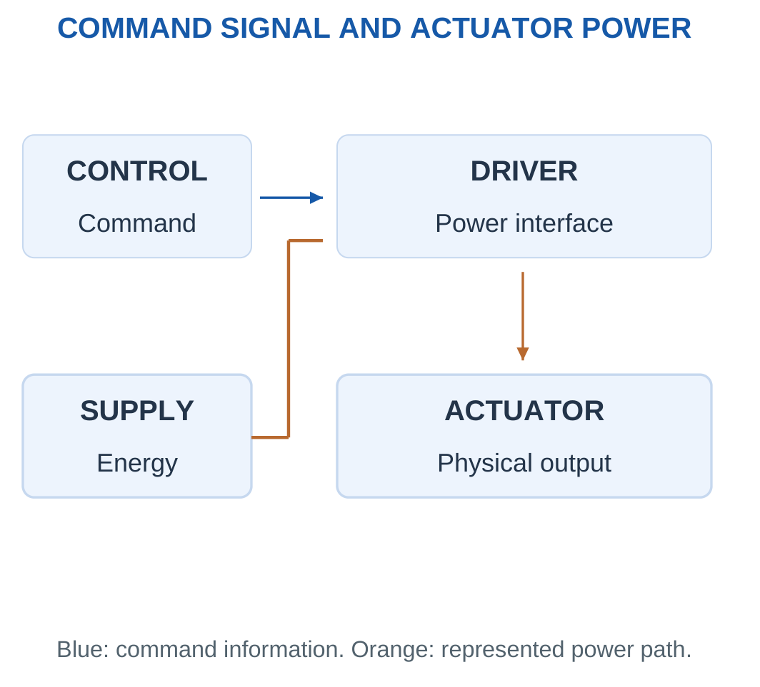
The controller determines an action using its task and measurements. A motor driver, ESC or controlled valve interfaces that decision with the relevant energy source.
The load receives mechanical power. Losses and stored-energy changes belong to the appropriate balance.
Electrical and Mechanical Power
For a stated DC electrical boundary:
Electrical input power = Voltage × Current
For rotary motion:
Mechanical power = Torque × Angular speed
For linear motion:
Mechanical power = Force × Linear speed
The quantities must describe the same physical boundary before an efficiency is formed.
Keeping Connections Distinct
A feedback wire reports information about motion. It is not the mechanical connection carrying the payload.
A communication network can coordinate machines without supplying their motor energy. A sensor signal can affect control action without becoming an additional energy source.
Worked Problem 5.3: Main Power and Command-Interface Power
Problem: A driver receives 24 V at 3 A. A separate command-interface example uses 5 V at 0.002 A. Calculate both powers and their ratio.
Solution:
Main input = 24 × 3 = 72 W
Command-interface power = 5 × 0.002 = 0.01 W
Ratio = 72 / 0.01 = 7200
Answer: Main input is 72 W, command-interface power is 0.01 W, and the ratio is 7200.
The comparison illustrates different roles. It is not the driver efficiency because the command-interface power is not the useful mechanical output.
Worked Problem 5.4: A Second Power Comparison
Problem: Main supply is 12 V at 4 A. The separate interface uses 3.3 V at 0.001 A.
Solution:
Main input = 12 × 4 = 48 W
Interface power = 3.3 × 0.001 = 0.0033 W
Ratio = 48 / 0.0033 = 14545.5
Answer: Powers are 48 W and 0.0033 W, with ratio approximately 14545.5.
The main supply delivers actuator energy, while the command communicates the requested action.
3. Sensors, Measurement and Signal Scaling
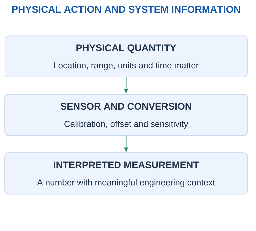
A sensor responds to a physical quantity and produces a usable signal. Position, speed, pressure, temperature and force can be measured through appropriate principles.
A controller needs the signal’s range, units, location, calibration and timing. A number without this context may be insufficient for a physical decision.

Linear Calibration
A supplied calibration can be written as:
Output = Offset + Sensitivity × Physical quantity
Therefore:
Physical quantity = (Output − Offset) / Sensitivity
The offset must be removed before dividing by sensitivity.
For:
V = 0.5 + 0.02x
a reading of 2.5 V gives:
x = (2.5 − 0.5) / 0.02 = 100 mm
Dividing 2.5 directly by 0.02 would incorrectly interpret the offset as displacement.
Resolution and Accuracy
Resolution describes a represented increment. Accuracy concerns agreement with the relevant reference.
A 0–100 mm span divided into 1000 equal intervals gives 0.1 mm per interval. This does not establish 0.1 mm accuracy because mounting, offset, nonlinearity and noise remain separate effects.
A converter model must also define whether its number refers to intervals, bins or endpoint-labelled levels.
Measurement Location
A motor-shaft encoder does not directly measure every elastic displacement of a remote tool.
A pressure measurement does not directly establish cylinder force without the relevant effective areas and load model.
Worked Problem 5.5: Position-Sensor Calibration
Problem: Vout = 0.5 + 0.02x, with volts and millimetres. Reading is 2.5 V. Find position and voltage change for another 5 mm.
Solution:
x = (2.5 − 0.5) / 0.02 = 100 mm
Voltage change = 0.02 × 5 = 0.1 V
Answer: Represented position is 100 mm, and the additional displacement produces 0.1 V change.
Worked Problem 5.6: A Different Sensor Slope
Problem: Vout = 1 + 0.01x and reading is 2.2 V.
Solution:
x = (2.2 − 1) / 0.01 = 120 mm
Change for 5 mm = 0.01 × 5 = 0.05 V
Answer: Position is 120 mm, and voltage change is 0.05 V.
Worked Problem 5.7: A Higher Sensitivity
Problem: Vout = 0.2 + 0.04x and reading is 3.4 V.
Solution:
x = (3.4 − 0.2) / 0.04 = 80 mm
Change for 5 mm = 0.04 × 5 = 0.2 V
Answer: Position is 80 mm, and voltage change is 0.2 V.
These are calibration results under the supplied linear model, not independent accuracy measurements.
4. Open-Loop and Closed-Loop Control
In an open-loop arrangement, control action does not use measured output feedback to correct the controlled quantity in the represented loop.
A command-counted stepper axis without continuous position feedback is an example. If motion is missed, the controller may continue to count commands without detecting the difference.
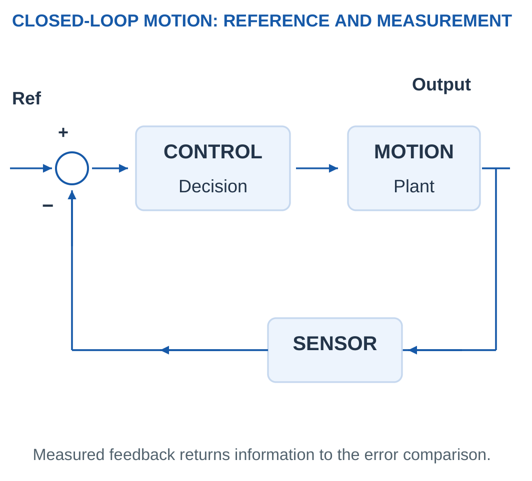
A closed-loop system measures a relevant output, compares it with the reference and adjusts its action according to a control rule.

Error Convention
Define:
Error = Reference − Measured output
A positive error means the measured value is below the reference under this convention.
A negative error means it exceeds the reference. The sign does not independently specify a universal motor-terminal polarity because installed directions and interfaces differ.
Proportional Model
A supplied arithmetic model can use:
u = K × Error
If the command has a limit, the applied model command must be restricted to that range.
Feedback alone does not guarantee stability, zero error or fast response. Sensors, delay, mechanics, controller design and actuator limits affect the result.
Worked Problem 5.8: Command Saturation
Problem: Reference is 100 mm, measurement 92 mm and K = 0.2 command units/mm. Command is limited to ±1.
Solution:
Error = 100 − 92 = 8 mm
Raw command = 0.2 × 8 = 1.6
The raw command exceeds +1.
Limited command = +1
Answer: Error is 8 mm, raw command is 1.6, and applied model command is 1.
Worked Problem 5.9: Negative Error
Problem: Reference is 50 mm, measurement 54 mm and K = 0.3. Limits are ±2.
Solution:
Error = 50 − 54 = −4 mm
Raw command = 0.3 × (−4) = −1.2
This lies within the limits.
Answer: Error is −4 mm, and both raw and limited commands are −1.2.
Worked Problem 5.10: Unsaturated Positive Command
Problem: Reference is 80 mm, measurement 79 mm and K = 0.5. Limits are ±1.
Solution:
Error = 1 mm
Raw command = 0.5 × 1 = 0.5
Limited command = 0.5
Answer: Error is 1 mm, and applied command is 0.5.
These examples calculate the specified rule. They do not demonstrate the complete dynamic response of an actual axis.
5. Actuators and Requirement-Based Selection
An actuator produces physical action. Electric motors commonly provide rotation. Cylinders commonly provide translation. A mechanism can convert and scale the action to match the load.
Actuator selection begins with the task rather than a preferred technology.

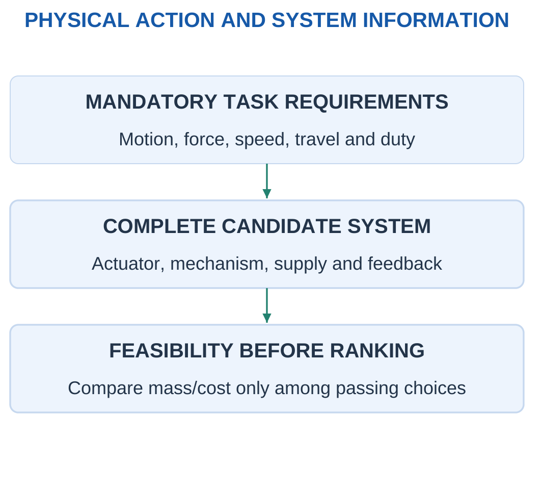
Required Information
- Motion type.
- Force or torque.
- Speed.
- Travel or rotation range.
- Continuous or intermittent duty.
- Available supply.
- Required feedback.
- Tool, adapter and payload.
- Mechanism and mounting arrangement.
Peak torque should not silently satisfy a continuous-torque requirement. A candidate that provides enough force but insufficient stroke fails an independent stroke requirement.
Complete-System Comparison
An electric option can require a motor, driver, screw and sensor. A hydraulic option can require a source, valve, cylinder and return path.
Mass and cost comparisons must include the explicitly represented complete systems.
Only candidates that meet all mandatory criteria should be ranked by mass, cost or another stated objective.
Worked Problem 5.11: Passing All Requirements
Problem: Required continuous force is 100 N, stroke 80 mm and speed 50 mm/s. Candidate limits are 150 N, 100 mm and 60 mm/s.
Solution:
150 ≥ 100 N: Pass
100 ≥ 80 mm: Pass
60 ≥ 50 mm/s: Pass
Answer: The candidate passes the three-condition screen.
This is an introductory feasibility result. Dynamic, thermal and installation requirements need their own information.
Worked Problem 5.12: Insufficient Stroke
Problem: Requirements are 120 N, 90 mm and 40 mm/s. Candidate limits are 200 N, 70 mm and 80 mm/s.
Solution:
Force and speed pass, but:
70 mm < 90 mm
Answer: The candidate fails because of insufficient stroke.
Extra force and speed do not compensate for a mandatory missing travel.
Worked Problem 5.13: Insufficient Speed
Problem: Requirements are 80 N, 60 mm and 70 mm/s. Candidate limits are 100 N, 80 mm and 50 mm/s.
Solution:
Force and stroke pass, but:
50 mm/s < 70 mm/s
Answer: The candidate fails the speed requirement.
6. DC Motors: Energy Conversion and Torque
A motor supplied from a DC source can convert electrical input into rotary mechanical action through current and magnetic-field interaction.
A basic brushed DC motor uses an armature, field, commutator and brushes. Brushless arrangements use electronic commutation and a different construction.

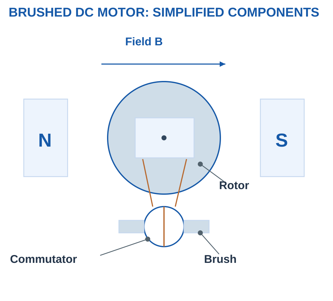
Simplified Armature Model
For the supplied steady model:
V = E + IR
where E is back EMF and IR is the represented resistance drop.
Back EMF = V − IR
A supplied torque constant gives:
Electromagnetic torque = kt × Current
Internal Conversion and Shaft Output
Electrical input = VI
Copper loss = I²R
Converted electromagnetic power = EI
Converted electromagnetic power is not automatically final shaft output. Additional mechanical losses may remain.
For V = 12 V, I = 2 A and R = 1 Ω:
E = 10 V
Input = 24 W
Copper loss = 4 W
Converted power = 20 W
If a further 3 W mechanical loss is supplied, shaft output becomes 17 W.
Worked Problem 5.14: Armature and Torque Model
Problem: V = 24 V, I = 2 A, R = 1 Ω and kt = 0.05 N m/A.
Solution:
E = 24 − 2 × 1 = 22 V
Torque = 0.05 × 2 = 0.1 N m
Copper loss = 2² × 1 = 4 W
Converted power = 22 × 2 = 44 W
Check: Input = 24 × 2 = 48 W = 44 + 4 W
Answer: Back EMF is 22 V, torque 0.1 N m, copper loss 4 W, and converted power 44 W.
Worked Problem 5.15: Another DC Motor Model
Problem: V = 12 V, I = 1.5 A, R = 0.8 Ω and kt = 0.04 N m/A.
Solution:
E = 12 − 1.5 × 0.8 = 10.8 V
Torque = 0.04 × 1.5 = 0.06 N m
Copper loss = 1.5² × 0.8 = 1.8 W
Converted power = 10.8 × 1.5 = 16.2 W
Answer: Back EMF is 10.8 V, torque 0.06 N m, copper loss 1.8 W, and converted power 16.2 W.
7. Motor Speed, Shaft Power and Losses
Rotational speed in rpm must be converted to angular speed before multiplying by torque.
Angular speed ω = 2πN / 60 rad/s
Shaft power = Shaft torque × Angular speed
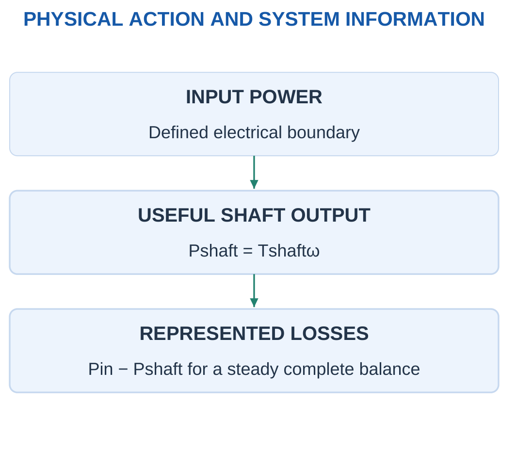
For a steady DC input:
Efficiency = Shaft output power / Electrical input power

At 300 rpm:
ω = 2π × 300 / 60 = 31.416 rad/s
For torque 0.2 N m:
Power = 0.2 × 31.416 = 6.283 W
Multiplying torque directly by 300 would mix rpm with rad/s.
Gear Reduction
For reduction:
r = Input speed / Output speed
With supplied gearbox efficiency η:
Output torque = η × Input torque × r
Torque increase accompanies reduced speed. A reduction does not create additional power.
Holding and Ratings
At zero speed, ideal mechanical output power is zero because angular speed is zero. Electrical input and heating need not be zero.
Continuous torque, peak torque, stall torque and no-load speed describe different conditions.
Worked Problem 5.16: Shaft Efficiency
Problem: Input is 24 V at 3 A. Shaft torque is 0.3 N m at 1500 rpm.
Solution:
Input = 72 W
ω = 2π × 1500 / 60 = 157.08 rad/s
Output = 0.3 × 157.08 = 47.1239 W
Efficiency = 47.1239 / 72 × 100 = 65.4498%
Loss = 72 − 47.1239 = 24.8761 W
Answer: Output is 47.1239 W, efficiency 65.4498%, and loss 24.8761 W.
Worked Problem 5.17: A Second Shaft-Power Calculation
Problem: Input is 12 V at 4 A. Torque is 0.2 N m at 1200 rpm.
Solution:
Input = 48 W
ω = 125.664 rad/s
Output = 25.1327 W
Efficiency = 52.3599%
Loss = 22.8673 W
Answer: Shaft output is 25.1327 W.
Worked Problem 5.18: A Higher-Voltage Boundary
Problem: Input is 48 V at 2 A. Torque is 0.45 N m at 1500 rpm.
Solution:
Input = 96 W
Output = 0.45 × 157.08 = 70.6858 W
Efficiency = 70.6858 / 96 × 100 = 73.6311%
Loss = 96 − 70.6858 = 25.3142 W
Answer: Output is 70.6858 W, efficiency 73.6311%, and loss 25.3142 W.
8. Drivers, Commands and Motion Mechanisms
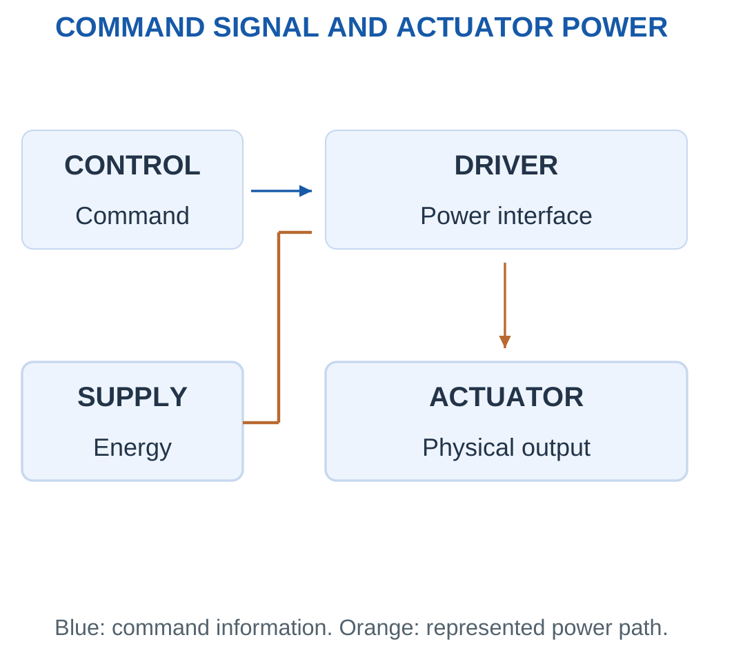
A driver receives a command and controls actuator power within its intended interface.
A command may influence a switched output, but actual speed depends on the supply, motor, load, driver and control arrangement.

Ideal Switching Average
For duty fraction D, supply Vs and a stated zero-voltage off level:
Average applied voltage = D × Vs
This is an electrical averaging model. It is not a universal motor-speed law.
A 25% duty model at 24 V gives 6 V average. It does not independently establish one-quarter of a loaded motor’s rated speed.
Mechanism Scaling
A screw converts relative turns into translation according to its lead.
A compatible timing pulley advances a belt by:
Travel per pulley revolution = Tooth count × Belt pitch
A gear reduction adds another explicitly defined scale.
Commanded position, shaft position and remote tool position can differ because of backlash, compliance, attachment and sensor location.
Worked Problem 5.19: Explicit Demonstration Mapping
Problem: Supply is 24 V and duty fraction 0.4. A separate demonstration map states N = Duty × 3000 rpm.
Solution:
Average voltage = 0.4 × 24 = 9.6 V
Mapped speed = 0.4 × 3000 = 1200 rpm
Answer: Average voltage is 9.6 V and speed under the supplied map is 1200 rpm.
The speed follows the explicitly given mapping rather than the voltage equation alone.
Worked Problem 5.20: Another Demonstration Mapping
Problem: Supply is 12 V and duty fraction 0.75. The separate map is N = Duty × 2000 rpm.
Solution:
Average voltage = 0.75 × 12 = 9 V
Mapped speed = 0.75 × 2000 = 1500 rpm
Answer: Average voltage is 9 V and mapped speed is 1500 rpm.
9. Stepper Motors and Discrete Command Increments
A stepper uses sequenced phase excitation to create nominal incremental rotor positions.
For full-step angle α:
Full steps per revolution = 360 / α
If the driver supplies m command subdivisions per full step:
Command increments per revolution = m × Full steps per revolution

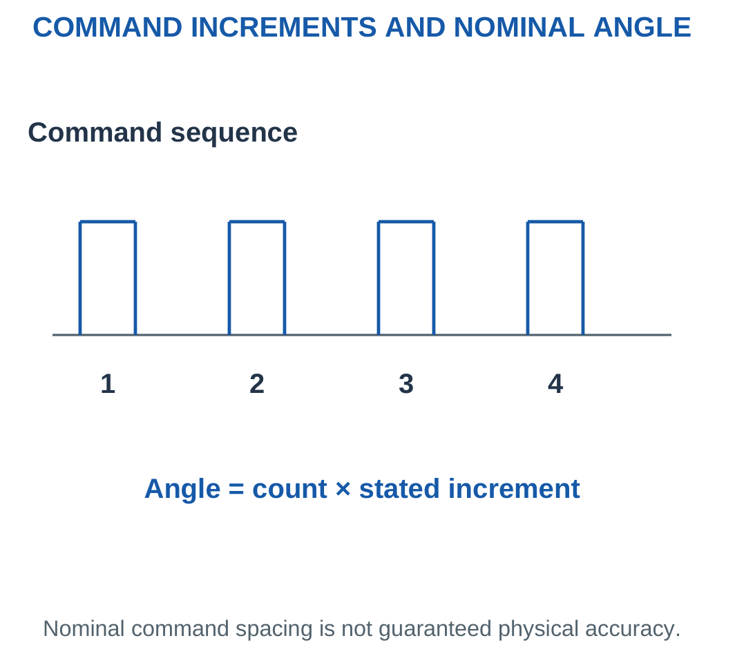
Microstepping
Microstepping subdivides phase-current commands. It creates finer command spacing but does not automatically create equal physical accuracy at every subdivision.
Actual behaviour depends on motor, driver, load and mechanics.
Missed Motion
A stepper can lose synchronism when the system cannot follow the requested load, speed or acceleration.
An open-loop controller may continue counting commands without observing the lost motion. Appropriate closed-loop stepper arrangements also exist.

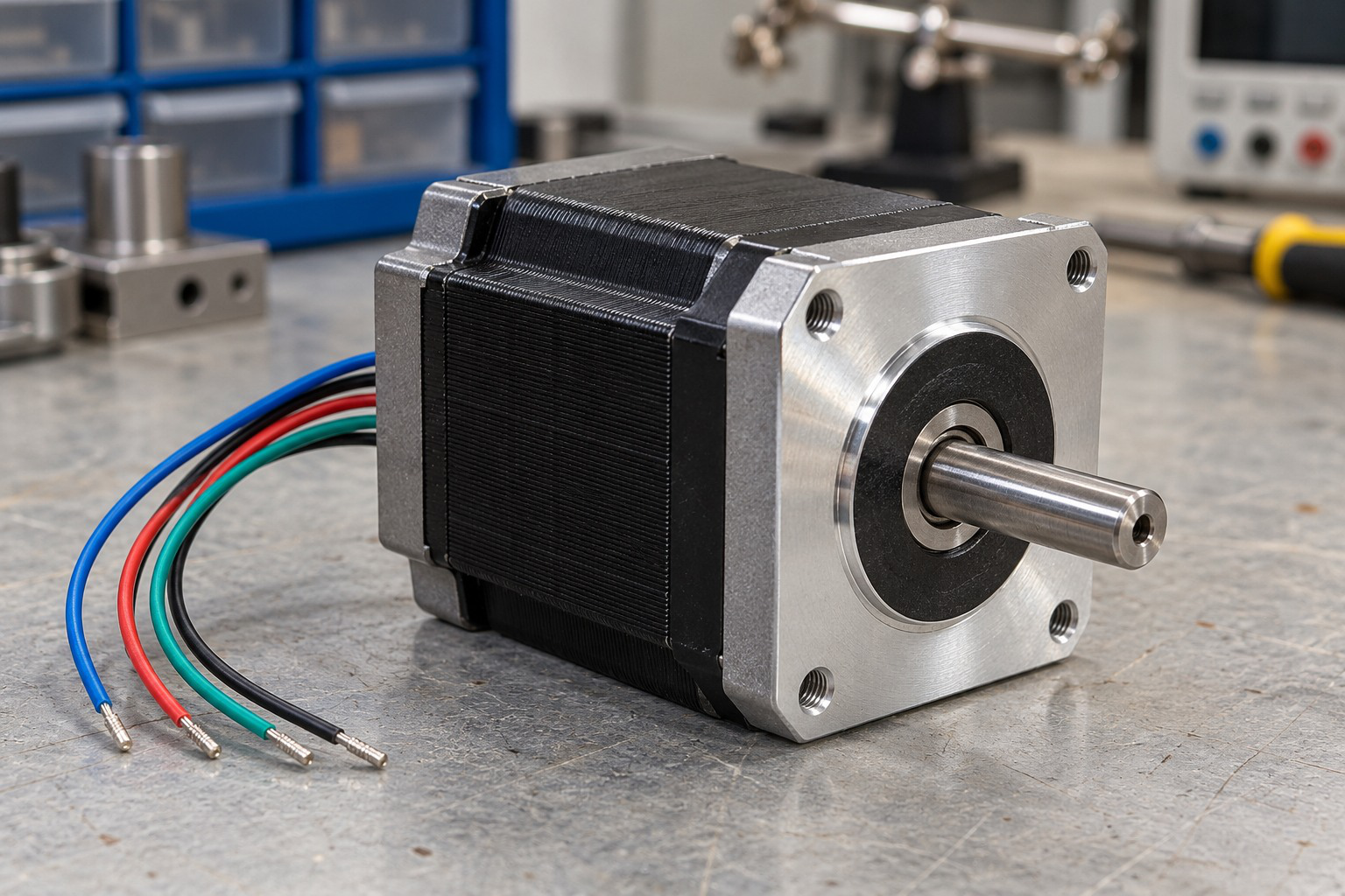
Worked Problem 5.21: Full Steps and Microstep Commands
Problem: Full-step angle is 0.9° and the driver supplies eight subdivisions per full step. Find full steps/revolution, command increments/revolution and commands for 45°.
Solution:
Full steps = 360 / 0.9 = 400
Command increments = 400 × 8 = 3200 per revolution
Nominal command spacing = 360 / 3200 = 0.1125°
Commands for 45° = 45 / 0.1125 = 400
Answer: 400 full steps/revolution, 3200 commands/revolution, and 400 commands for the move.
Worked Problem 5.22: A 1.8° Stepper
Problem: Full-step angle is 1.8° with eight subdivisions. Find commands for 180°.
Solution:
Full steps = 360 / 1.8 = 200
Commands/revolution = 200 × 8 = 1600
Spacing = 360 / 1600 = 0.225°
Commands = 180 / 0.225 = 800
Answer: 200 full steps/revolution, 1600 commands/revolution, and 800 commands for 180°.
These are nominal command calculations under the followed-motion assumption.
10. Stepper Pulses, Speed and Linear Travel
If S command increments correspond to one motor revolution and command frequency is fp increments/s:
Motor speed = 60fp / S rpm
For a direct screw with lead l:
Travel per command = l / S
Commands for distance x = xS / l
Linear speed = fp × l / S

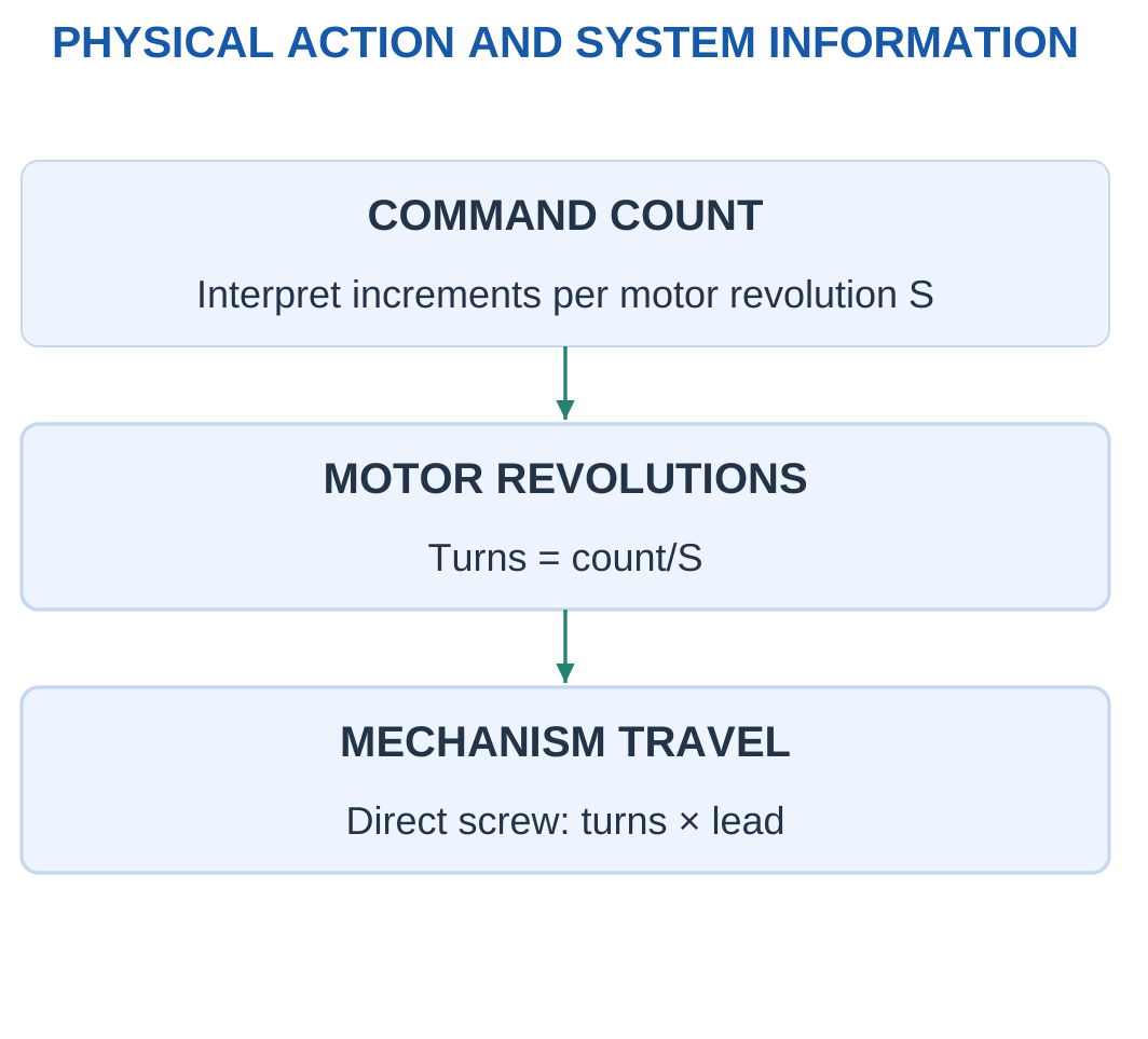
These relationships assume that commands are followed. They omit backlash, missed steps, elasticity and acceleration unless supplied separately.
Unit Check
Commands per second divided by commands per revolution gives revolutions per second.
Multiplying by lead in millimetres per revolution then gives millimetres per second.
A belt axis uses the pulley’s travel per turn instead of screw lead.
Worked Problem 5.23: A 4 mm Lead Axis
Problem: Lead is 4 mm/rev and command basis is 3200 increments/rev. Find commands for 40 mm and motion at 6400 increments/s.
Solution:
Commands = 40 × 3200 / 4 = 32000
Motor speed = 60 × 6400 / 3200 = 120 rpm
Linear speed = 6400 × 4 / 3200 = 8 mm/s
Time = 40 / 8 = 5 s
Answer: 32000 commands, 120 rpm, 8 mm/s, and 5 s.
Worked Problem 5.24: A 2 mm Lead Axis
Problem: Lead is 2 mm/rev, command basis 1600/rev, travel 30 mm and frequency 4000/s.
Solution:
Commands = 30 × 1600 / 2 = 24000
Speed = 60 × 4000 / 1600 = 150 rpm
Linear speed = 4000 × 2 / 1600 = 5 mm/s
Time = 30 / 5 = 6 s
Answer: 24000 commands, 150 rpm, 5 mm/s, and 6 s.
Worked Problem 5.25: An 8 mm Lead Axis
Problem: Lead is 8 mm/rev, command basis 3200/rev, travel 80 mm and frequency 8000/s.
Solution:
Commands = 80 × 3200 / 8 = 32000
Speed = 150 rpm
Linear speed = 8000 × 8 / 3200 = 20 mm/s
Time = 80 / 20 = 4 s
Answer: 32000 commands, 150 rpm, 20 mm/s, and 4 s.
11. Servo Systems: Reference, Error and Feedback
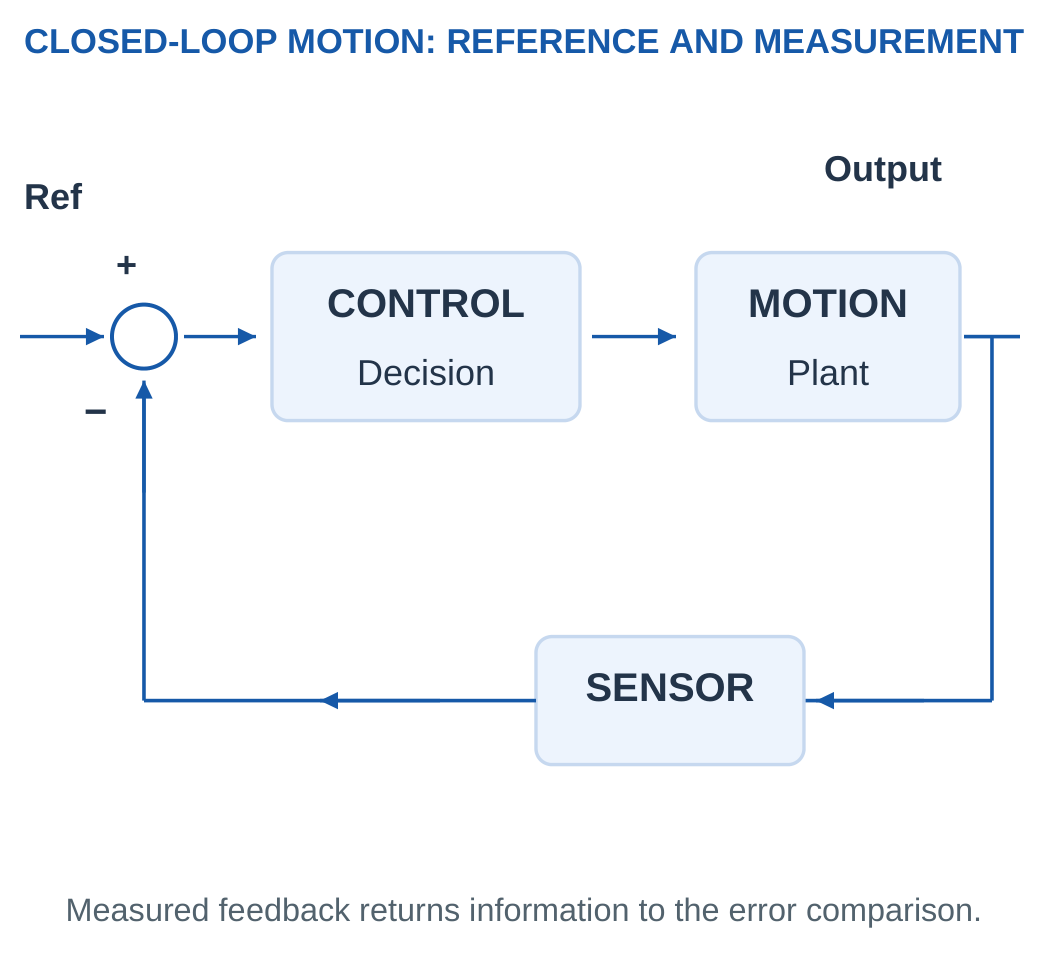
A servo controls motion using feedback about a relevant quantity such as position, speed or torque.
Its essential elements include a reference, controller, power drive, actuator and measurement path.
“Servo” describes a controlled arrangement rather than one universal motor construction or angular range.

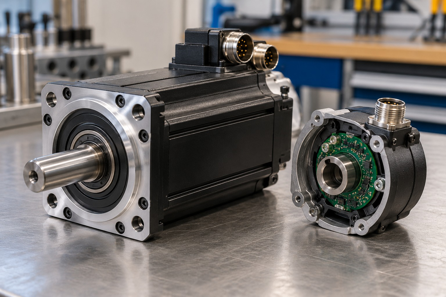
A small integrated servo may contain gears, a motor, sensor and electronics. An industrial axis may use different components and interfaces.
Their command protocols and limits cannot be assumed identical because both are called servos.
Error and Measurement Location
Use:
Error = Reference angle − Measured angle
A motor-shaft sensor does not necessarily observe remote tool deflection or backlash.
Actuator saturation, delay and mechanical constraints also limit the achievable response.
Worked Problem 5.26: A Supplied Command Map
Problem: Command 0 represents 0° and command 100 represents 180°. At command 25, measured output is 42°.
Solution:
Reference angle = 25 × 180 / 100 = 45°
Error = 45 − 42 = 3°
Answer: Reference is 45° and signed error is +3°.
The supplied linear mapping is an exercise definition rather than a universal servo command specification.

Worked Problem 5.27: A Map with Command Offset
Problem: Command 10 represents 0° and command 110 represents 120°. At command 60, output is measured as 58°.
Solution:
The command span is 100 units and the selected command is 50 units above its zero-angle reference.
Reference = (60 − 10) × 120 / 100 = 60°
Error = 60 − 58 = 2°
Answer: Reference is 60° and signed error is +2°.
12. Encoders, Counts and Represented Position
An encoder provides position or motion information according to its sensing principle and interface.
An incremental encoder reports changes relative to a reference process. An absolute encoder reports a coded position within its defined range.

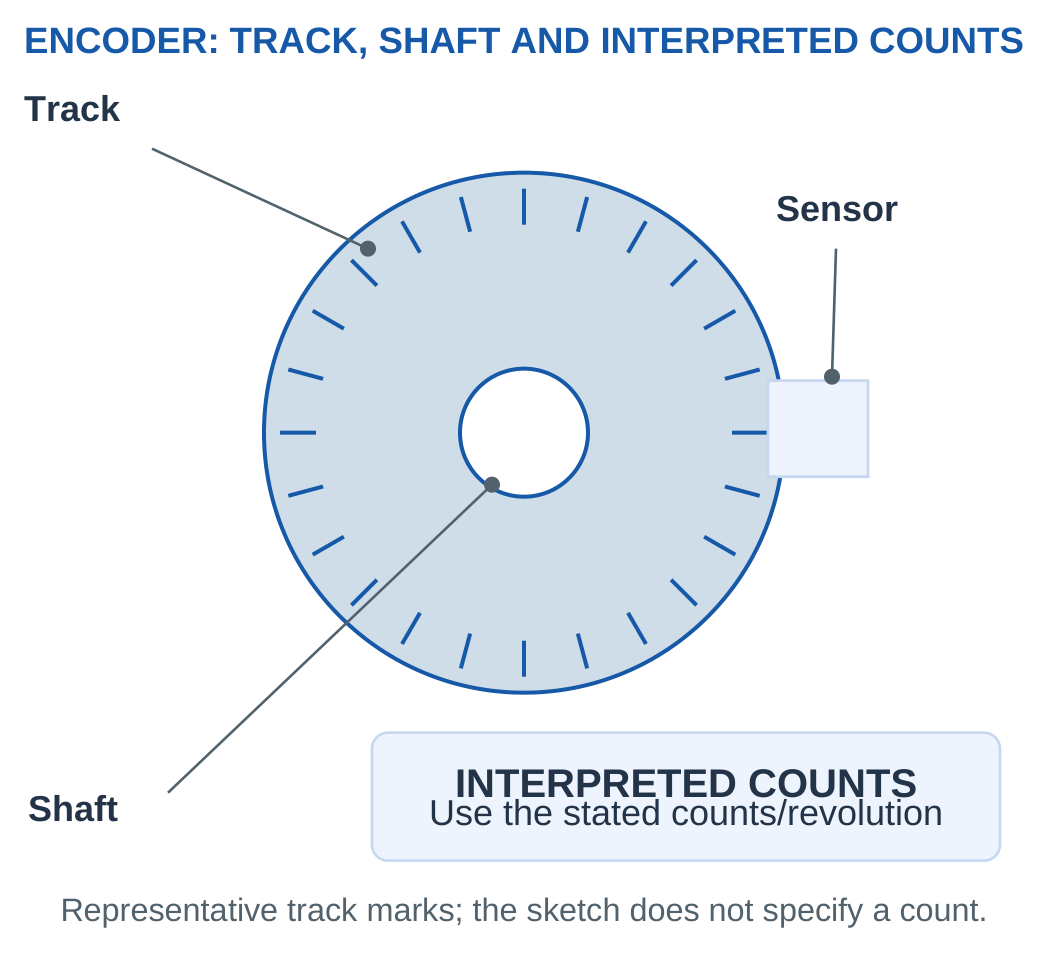
For C interpreted counts per revolution:
Nominal angular spacing = 360 / C degrees
Relative angle = Count change × 360 / C
Quadrature decoding can change the interpreted counts per cycle. If the supplied count already includes decoding, multiplying it again would be incorrect.
Resolution and Tool Accuracy
A high count number does not eliminate offset, attachment error, quantisation or transmission compliance.
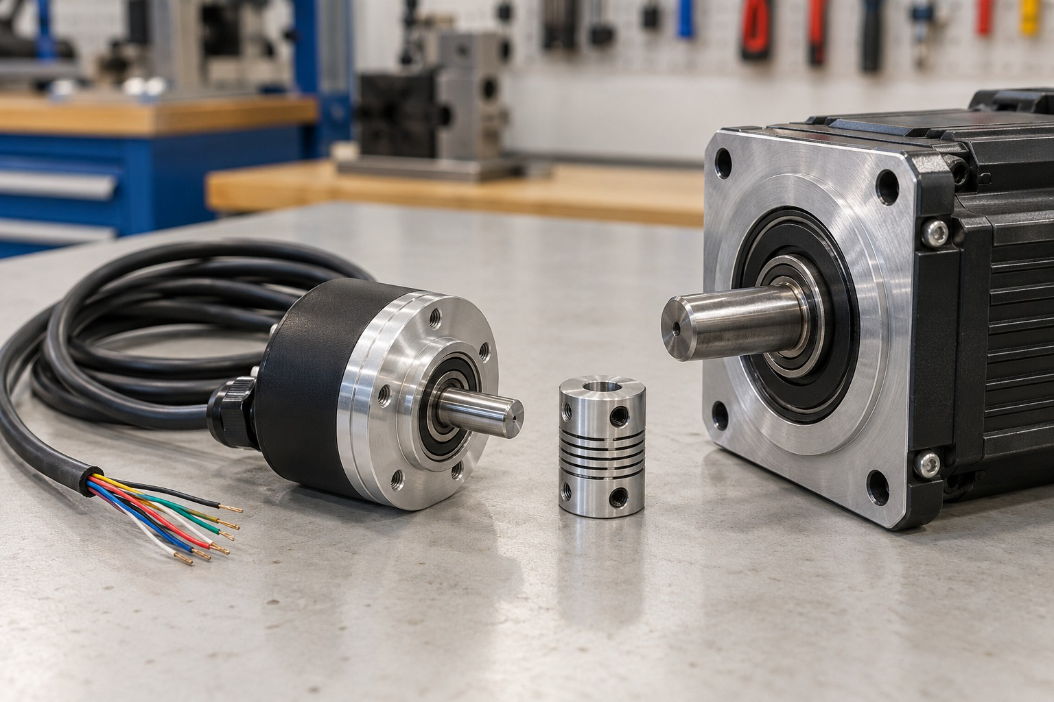
The sensor measures at its installed location. A remote tool can have additional backlash or elastic motion.
Average Speed
For count change n during interval Δt:
Average speed = 60n / (CΔt) rpm
This is an interval average under the stated count and direction interpretation.

Worked Problem 5.28: Counts and Average Speed
Problem: Encoder has 2000 interpreted counts/revolution. A positive change of 250 counts occurs in 0.2 s without unknown wrap or extra turns.
Solution:
Spacing = 360 / 2000 = 0.18°
Angle = 250 × 0.18 = 45°
Speed = 60 × 250 / (2000 × 0.2) = 37.5 rpm
Answer: Spacing is 0.18°, angle 45°, and average speed 37.5 rpm.
Worked Problem 5.29: Another Encoder Basis
Problem: Encoder has 3600 interpreted counts/revolution. A positive change of 900 occurs in 0.25 s.
Solution:
Spacing = 0.1°
Angle = 900 × 0.1 = 90°
Speed = 60 × 900 / (3600 × 0.25) = 60 rpm
Answer: Spacing is 0.1°, angle 90°, and average speed 60 rpm.
13. Hydraulic Actuation and Fluid-Power Components
Hydraulic actuation uses suitable pressurised liquid to transmit power.
A basic system includes a reservoir, pump, appropriate pressure-control devices, directional valve, actuator and return path.
The pump supplies flow. Pressure develops according to load and restrictions within the operating system.

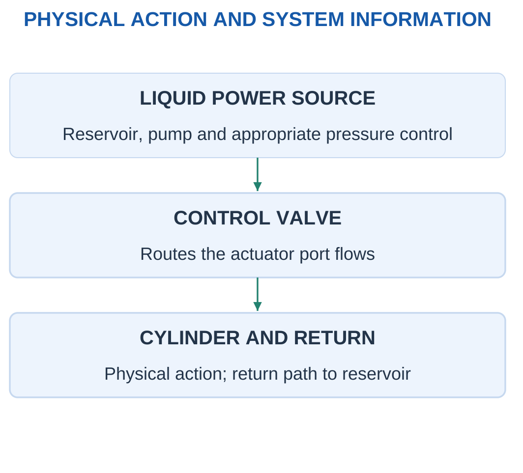
A cylinder creates linear action. A hydraulic motor creates rotation.
The liquid is often treated as approximately incompressible in elementary calculations. Real leakage, compliance, friction and line losses remain possible.
Power and Control
A valve command controls routing while the source supplies energy. The electrical signal to the valve is different from the fluid-power path to the cylinder.
High force through suitable pressure and area does not remove the need to consider contamination, seals, temperature and load holding.
Hydraulic Power
For a defined pressure rise and corresponding flow:
Hydraulic power = Pressure rise × Flow rate
Pressure in pascals and flow in m³/s give watts.
Worked Problem 5.30: Source Power and Efficiency
Problem: Pressure rise is 5 MPa and flow 2 L/min. Input-to-hydraulic-output efficiency is 0.8.
Solution:
Flow = 2 × 0.001 / 60 = 0.0000333333 m³/s
Hydraulic output = 5,000,000 × 0.0000333333 = 166.667 W
Input power = 166.667 / 0.8 = 208.333 W
Loss = 208.333 − 166.667 = 41.6667 W
Answer: Hydraulic output is 166.667 W, input 208.333 W, and loss 41.6667 W.

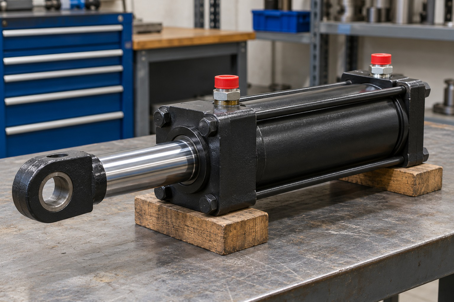
14. Hydraulic-Cylinder Areas and Ideal Force
For bore D and rod diameter d:
Cap-end area Ac = πD² / 4
Rod-side annular area Aa = π(D² − d²) / 4
The rod occupies part of the section, so the annular area is smaller than the full bore area.

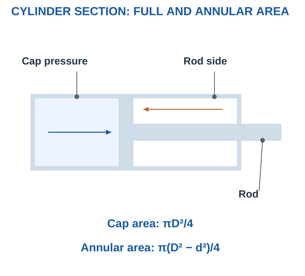
With extension positive:
Pressure force = Cap pressure × Cap area − Rod pressure × Annular area
If known friction resists extension:
Available extension force = Pressure force − Resisting friction
The pressure reference must be consistent. MPa multiplied by mm² gives newtons because:
1 MPa = 1 N/mm²
Worked Problem 5.31: Extension with Backpressure
Problem: Bore is 40 mm, rod 20 mm, cap pressure 5 MPa, rod pressure 0.5 MPa and resisting friction 100 N.
Solution:
Ac = π × 40² / 4 = 1256.64 mm²
Aa = π × (40² − 20²) / 4 = 942.478 mm²
Force = 5 × 1256.64 − 0.5 × 942.478 − 100
Force = 5711.95 N
Answer: Areas are 1256.64 mm² and 942.478 mm²; available extension estimate is 5711.95 N.
Worked Problem 5.32: A Larger Cylinder
Problem: Bore 50 mm, rod 25 mm, pressures 4 and 0.4 MPa, friction 150 N.
Solution:
Ac = 1963.5 mm²
Aa = 1472.62 mm²
Force = 4 × 1963.5 − 0.4 × 1472.62 − 150
Force = 7114.93 N
Answer: Available extension estimate is 7114.93 N.
Worked Problem 5.33: A Smaller Bore
Problem: Bore 32 mm, rod 16 mm, cap pressure 6 MPa, rod pressure 0.3 MPa and friction 80 N.
Solution:
Ac = 804.248 mm²
Aa = 603.186 mm²
Force = 6 × 804.248 − 0.3 × 603.186 − 80
Force = 4564.53 N
Answer: Available extension estimate is 4564.53 N.
Omitting rod-side pressure would overstate the represented force in these examples.
15. Hydraulic Flow, Speed and Power
For a supplied local chamber-flow model:
Speed = Flow / Effective area
Swept volume = Effective area × Stroke
Stroke time = Swept volume / Flow
The chamber must be named. Cap-end extension uses the full bore area. Rod-end retraction uses the annular area.

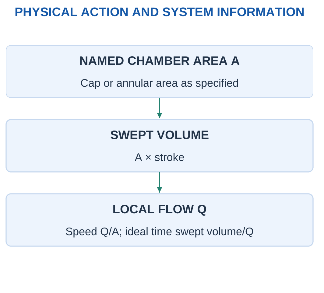
With the same local flow, a smaller effective area gives higher ideal speed.
Under matching ideal one-sided conditions:
Mechanical power = Force × Speed = Pressure × Flow
This provides an independent check. It should not combine force from one condition with speed from another.
Worked Problem 5.34: Extension Speed and Power
Problem: Bore 40 mm, cap flow 2 L/min, stroke 100 mm and one-sided pressure 5 MPa. Opposing gauge pressure and friction are zero.
Solution:
Area = 1256.64 mm²
Flow = 33333.3 mm³/s
Speed = 33333.3 / 1256.64 = 26.5258 mm/s
Time = 100 / 26.5258 = 3.76991 s
Force = 5 × 1256.64 = 6283.19 N
Power = 6283.19 × 0.0265258 = 166.667 W
Answer: Speed 26.5258 mm/s, time 3.76991 s, force 6283.19 N, power 166.667 W.
Worked Problem 5.35: A 50 mm Bore
Problem: Bore 50 mm, flow 3 L/min, stroke 150 mm and one-sided pressure 4 MPa.
Solution:
Area = 1963.5 mm²
Flow = 50000 mm³/s
Speed = 25.4648 mm/s
Time = 150 / 25.4648 = 5.89049 s
Force = 4 × 1963.5 = 7853.98 N
Power = 200 W
Answer: Speed 25.4648 mm/s, time 5.89049 s, force 7853.98 N, power 200 W.
Worked Problem 5.36: A 32 mm Bore
Problem: Bore 32 mm, flow 1.5 L/min, stroke 80 mm and pressure 6 MPa.
Solution:
Area = 804.248 mm²
Flow = 25000 mm³/s
Speed = 31.0849 mm/s
Time = 2.57359 s
Force = 4825.49 N
Power = 150 W
Answer: The ideal model gives 31.0849 mm/s, 2.57359 s, 4825.49 N and 150 W.
16. Pneumatic Actuation and Compressed Air
Pneumatic systems use compressed gas, commonly air, to produce physical action.
A conceptual arrangement includes a compressed-air source, suitable conditioning and regulation, valves, actuator and exhaust paths.

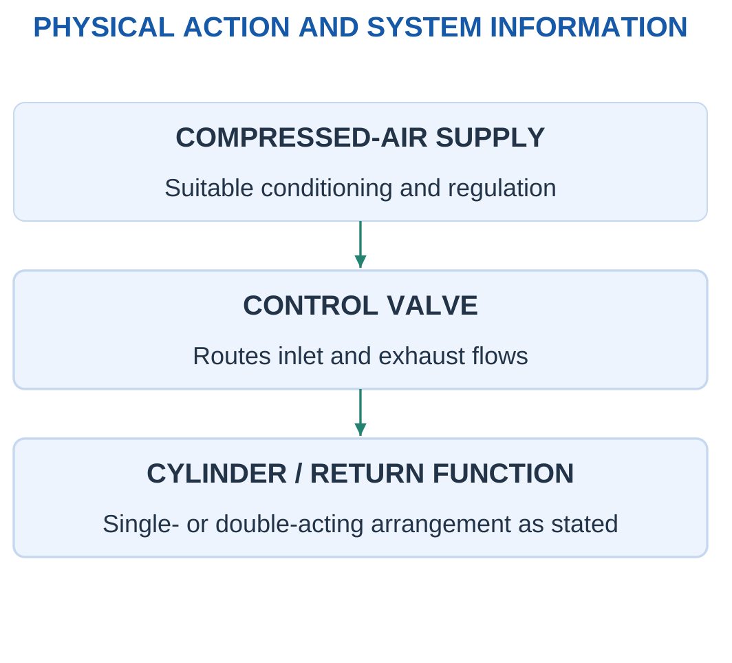
Air compressibility affects stiffness, response and flow interpretation. It should not be treated as an incompressible liquid without the stated approximation.
A single-acting cylinder can use pressure in one direction with spring or another return arrangement. A double-acting cylinder uses controlled pressure on the relevant sides.
Flow Reference
Gas volume depends on pressure and temperature.
A standard-condition air-flow value is not automatically the local pressurised chamber volume flow needed for Q/A.
The reference must be stated before using a volumetric rate to calculate speed.
Worked Problem 5.37: Pneumatic Handling Cycle
Problem: A 100 mm stroke takes 0.5 s to extend and 0.5 s to retract. There is a 0.2 s dwell at each end.
Solution:
Mean moving speed = 100 / 0.5 = 200 mm/s
Cycle time = 0.5 + 0.2 + 0.5 + 0.2 = 1.4 s
Ideal cycles/min = 60 / 1.4 = 42.8571
Answer: Mean moving speed is 200 mm/s, cycle time 1.4 s, and ideal rate 42.8571 cycles/min.
The moving speed is an interval average, not proof of a constant instantaneous speed.


17. Pneumatic Force and Practical Force Margins
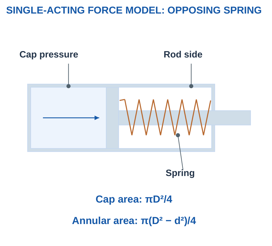
For a single-acting cap-end model with stated zero-gauge rod-side reference:
Pressure force = Gauge pressure × Cap area
If spring and friction oppose extension:
Available force = Pressure force − Spring force − Friction

Unit Conversion
1 bar = 0.1 MPa
Pressure in MPa can be multiplied directly by area in mm² to obtain newtons.
The supplied static model does not automatically account for pressure change during movement, acceleration or complete flow behaviour.
Worked Problem 5.38: Passing Force Requirement
Problem: Bore 32 mm, supply 6 bar gauge, spring force 80 N and friction 20 N. Required output is 300 N.
Solution:
Pressure = 0.6 MPa
Area = π × 32² / 4 = 804.248 mm²
Pressure force = 0.6 × 804.248 = 482.549 N
Available force = 482.549 − 80 − 20 = 382.549 N
382.549 ≥ 300 N
Answer: Available force is 382.549 N and the stated static screen passes.
Worked Problem 5.39: Failing Force Requirement
Problem: Bore 25 mm, pressure 5 bar, spring 40 N, friction 15 N and requirement 220 N.
Solution:
Area = 490.874 mm²
Pressure force = 0.5 × 490.874 = 245.437 N
Available force = 245.437 − 40 − 15 = 190.437 N
190.437 < 220 N
Answer: Available force is 190.437 N and the screen fails.
Worked Problem 5.40: A Larger Cylinder
Problem: Bore 40 mm, pressure 4 bar, spring 100 N, friction 30 N and requirement 350 N.
Solution:
Area = 1256.64 mm²
Pressure force = 0.4 × 1256.64 = 502.655 N
Available force = 502.655 − 100 − 30 = 372.655 N
Answer: Available force is 372.655 N and the screen passes.
18. Comparing Actuator Systems by the Task
Actuator comparison should use the actual task and complete represented system.
An electric axis, hydraulic cylinder and pneumatic mechanism have different supply, control and mechanical requirements.
A technology label alone does not establish the best choice.

Selection Order
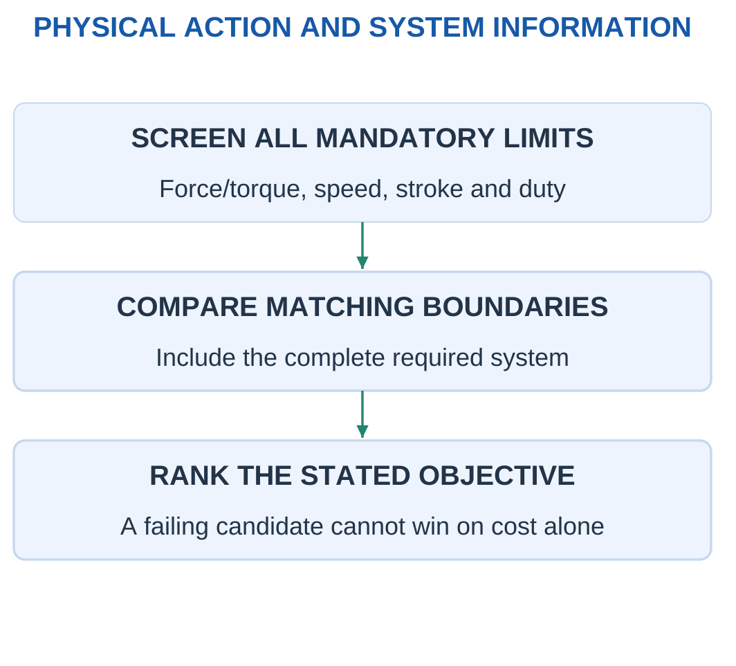
First define mandatory force or torque, speed, travel, duty and feedback.
Next check every candidate using matching operating definitions.
Then rank only the passing candidates by the stated objective.
A peak rating must not be compared with a continuous requirement as though they were the same condition.
The lightest feasible choice and lowest-cost feasible choice may be different.
Worked Problem 5.41: Feasible Ranking
Problem: Pass status for A/B/C is pass/fail/pass. Complete masses are 4/3/5 kg and costs are 100/120/90 units.
Solution:
B is excluded because it fails the mandatory screen.
Among A and C:
- A is lighter: 4 kg versus 5 kg.
- C is cheaper: 90 versus 100 units.
Answer: Lightest feasible choice is A. Lowest-cost feasible choice is C.
Worked Problem 5.42: Another Candidate Set
Problem: Pass status is fail/pass/pass. Masses are 6/4/3 kg and costs 150/170/190 units.
Solution:
A is excluded.
Among B and C:
- C is lighter at 3 kg.
- B is cheaper at 170 units.
Answer: Lightest feasible choice is C. Lowest-cost feasible choice is B.
A failing candidate cannot win solely because one secondary property is favourable.
19. Robots, Joints, Links and Degrees of Freedom
A robot mechanism consists of links connected by joints, with actuation and control arranged to perform a task.
A revolute joint provides rotation about an axis. A prismatic joint provides translation along an axis.

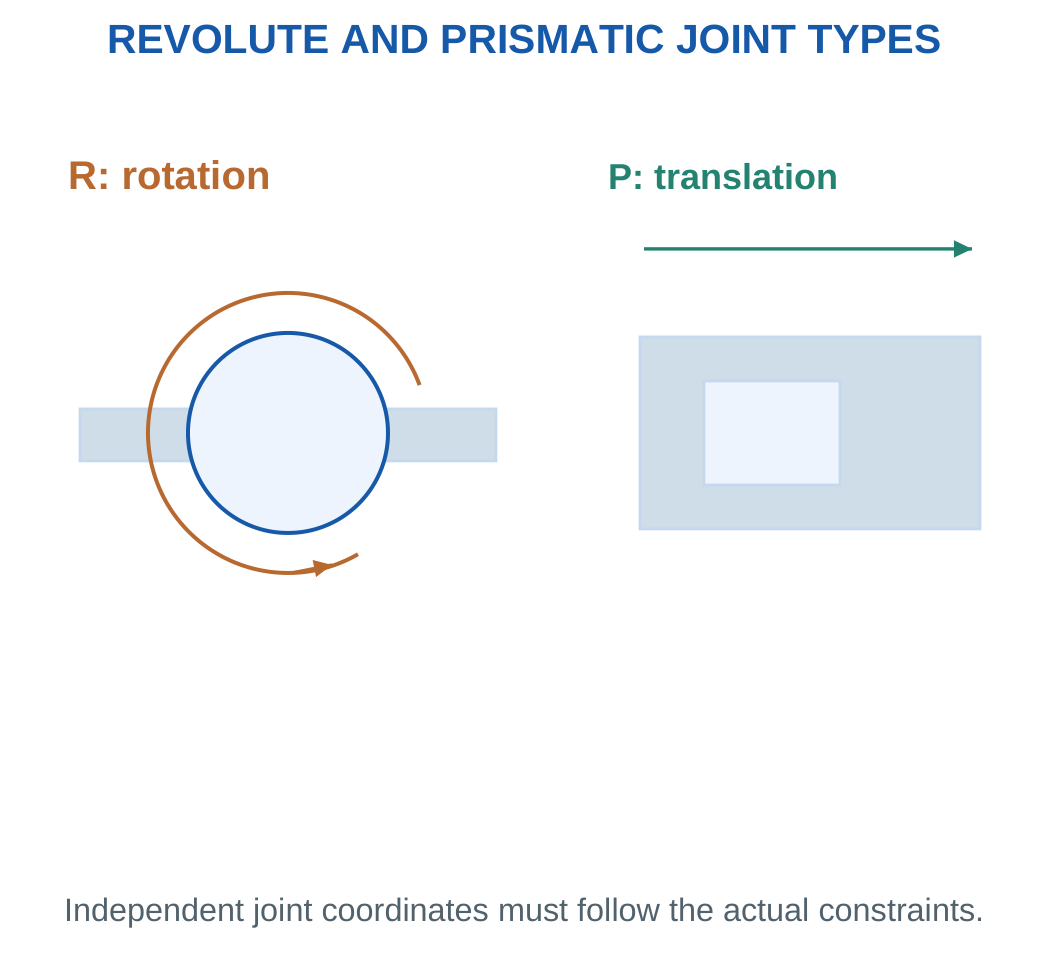
Degrees of freedom describe independent coordinates needed for the represented motion.
Counting motors or visible components does not always give the correct number because coordinates may be coupled or constrained.
Arm and Gripper Boundaries
A robot arm’s position and orientation coordinates can be counted separately from a gripper’s opening coordinate.
The question must specify whether the gripper is included.
A complete spatial task may require both position and orientation. Reaching a point does not automatically establish every possible tool orientation there.
Worked Problem 5.43: Three Prismatic Coordinates
Problem: A model has three independent prismatic arm coordinates, no revolute arm coordinates and a separate gripper opening coordinate.
Solution:
Arm-only count = 3
Arm-plus-gripper count = 3 + 1 = 4
Answer: Counts are 3 and 4.
Worked Problem 5.44: Mixed Joint Coordinates
Problem: A model has one independent prismatic and three independent revolute arm coordinates. The gripper adds one independent opening coordinate.
Solution:
Arm count = 1 + 3 = 4
Including gripper = 4 + 1 = 5
Answer: Counts are 4 and 5.
Worked Problem 5.45: Six Revolute Coordinates
Problem: A model has six independent revolute arm coordinates and a separate gripper coordinate.
Solution:
Arm-only count = 6
Including gripper = 7
Answer: Counts are 6 and 7.
These counts follow the explicit independence and no-coupling assumptions.
20. Cartesian Robots and Orthogonal Linear Axes
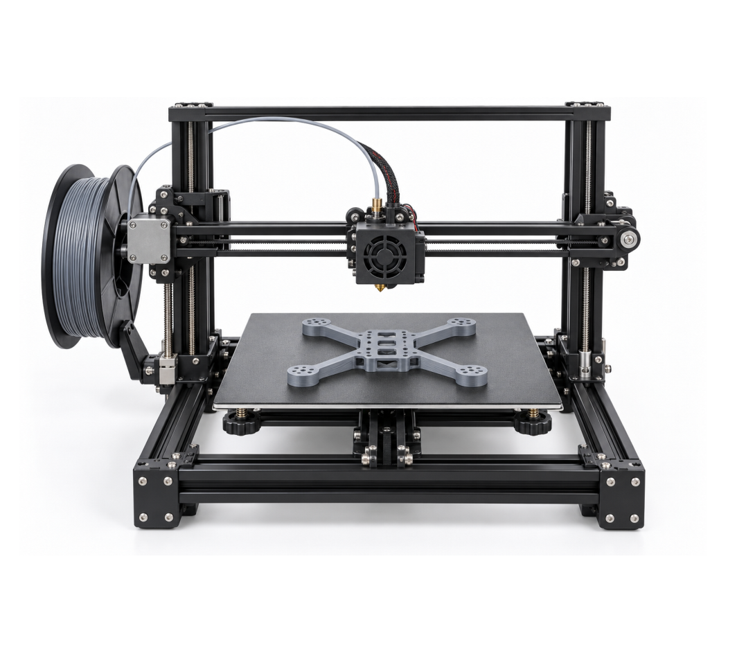
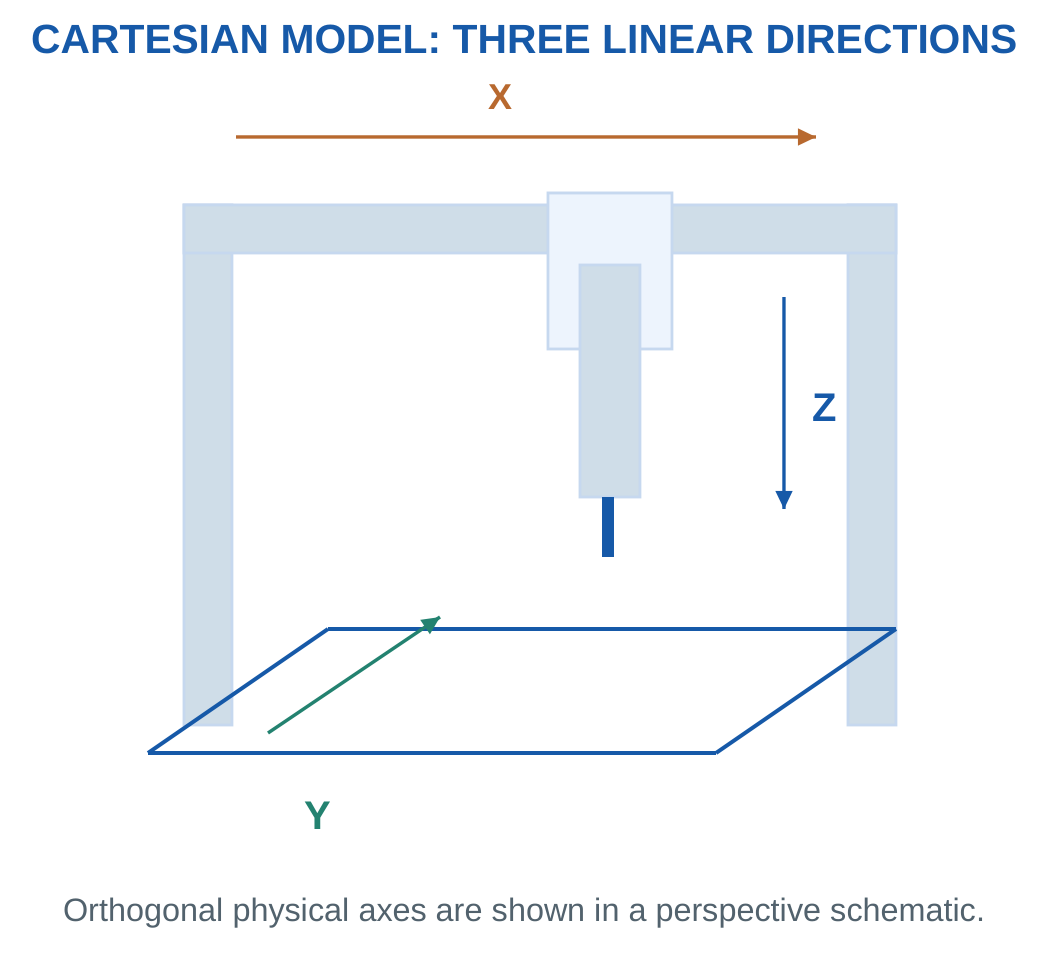
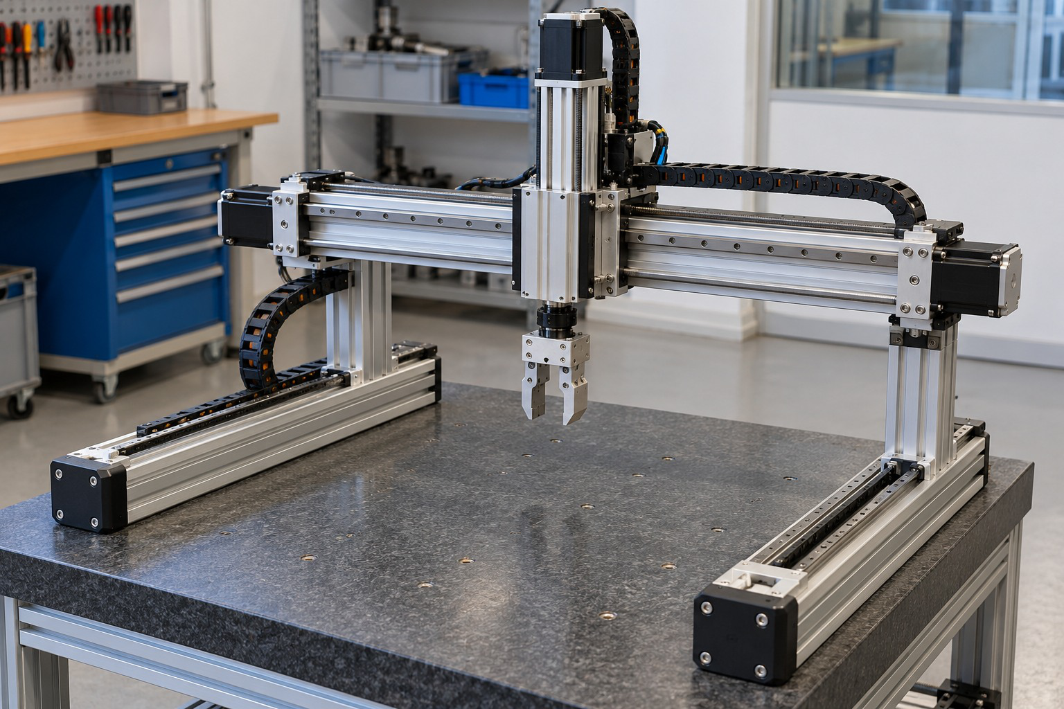
A Cartesian arrangement uses orthogonal linear directions, commonly described as X, Y and Z.
The geometry provides a direct relationship between axis travel and tool translation.
A printer or gantry can illustrate these directions, although the specific machine’s purpose and full construction must still be identified.



Ideal Travel Box
For independent travel lengths X, Y and Z:
Geometric travel-box volume = X × Y × Z
The box is not a complete collision-free workspace. Tools, fixtures, orientation and surrounding equipment can restrict usable access.
Worked Problem 5.46: Point and Volume Screen
Problem: Inclusive travels are X = 0–400, Y = 0–300 and Z = 0–200 mm. Check point (250, 150, 100) mm and calculate volume.
Solution:
Every coordinate lies within its stated range.
Volume = 400 × 300 × 200 = 24000000 mm³
Volume = 24000000 / 1000000000 = 0.024 m³
Answer: Point screen passes and geometric volume is 0.024 m³.

Worked Problem 5.47: Point Outside One Axis
Problem: Travels are 0–500, 0–200 and 0–100 mm. Check point (400, 180, 110) mm.
Solution:
X and Y lie within their ranges. Z = 110 mm exceeds 100 mm.
Volume = 500 × 200 × 100 = 10000000 mm³ = 0.01 m³
Answer: Point screen fails and volume is 0.01 m³.
21. SCARA Robots and Planar-Link Motion
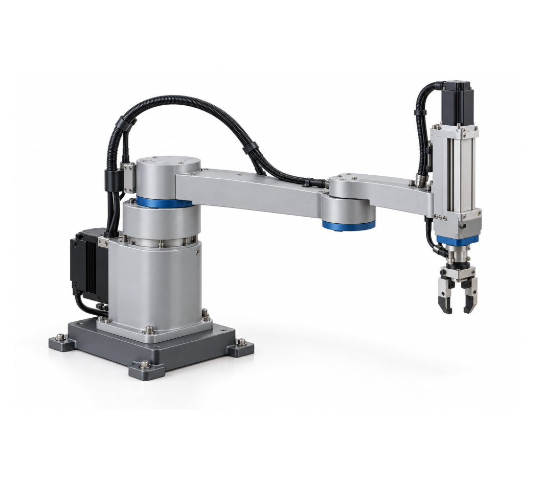
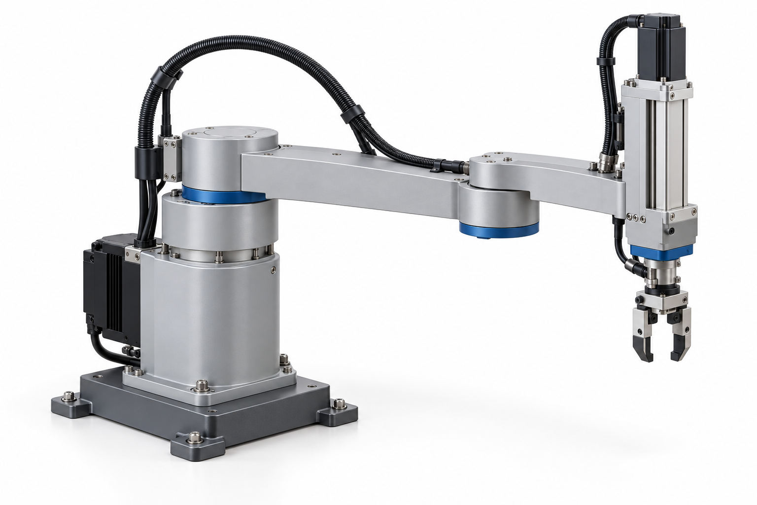
A common SCARA arrangement uses two planar rotary links with additional vertical and tool-axis motion.
Its geometry is useful for suitable assembly and handling tasks. Actual axis count, limits, stiffness and performance depend on the design.



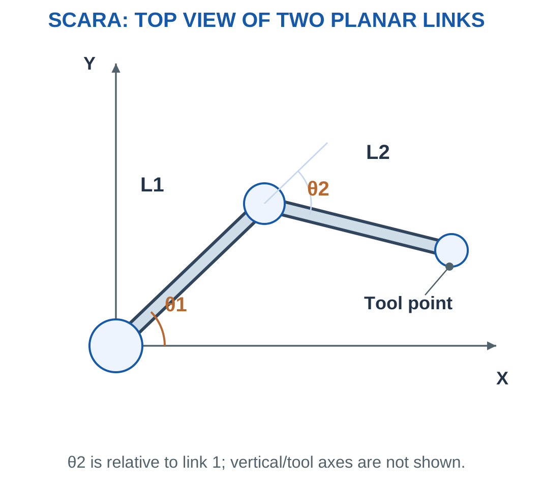
For first angle θ1 and second relative angle θ2:
x = L1 cos θ1 + L2 cos(θ1 + θ2)
y = L1 sin θ1 + L2 sin(θ1 + θ2)
Radial distance = √(x² + y²)
Ignoring limits and collisions, ideal radial reach lies between:
Minimum radius = |L1 − L2|
Maximum radius = L1 + L2
Worked Problem 5.48: Two-Link Endpoint
Problem: L1 = 200 mm, L2 = 150 mm, θ1 = 30° and relative θ2 = 60°.
Solution:
Second-link global angle = 30° + 60° = 90°
x = 200 cos 30° + 150 cos 90° = 173.205 mm
y = 200 sin 30° + 150 sin 90° = 250 mm
Radius = 304.138 mm
Answer: Endpoint is (173.205, 250) mm and radius 304.138 mm.
Worked Problem 5.49: Orthogonal Link Directions
Problem: L1 = 250 mm, L2 = 100 mm, θ1 = 0° and θ2 = 90°.
Solution:
x = 250 mm
y = 100 mm
Radius = √(250² + 100²) = 269.258 mm
Answer: Endpoint is (250, 100) mm.
Worked Problem 5.50: Negative Relative Angle
Problem: L1 = 150 mm, L2 = 100 mm, θ1 = 45° and θ2 = −90°.
Solution:
Second-link global angle = −45°
x = 150 cos 45° + 100 cos(−45°) = 176.777 mm
y = 150 sin 45° + 100 sin(−45°) = 35.3553 mm
Radius = 180.278 mm
Answer: Endpoint is (176.777, 35.3553) mm.
22. Articulated Robots and Jointed Motion
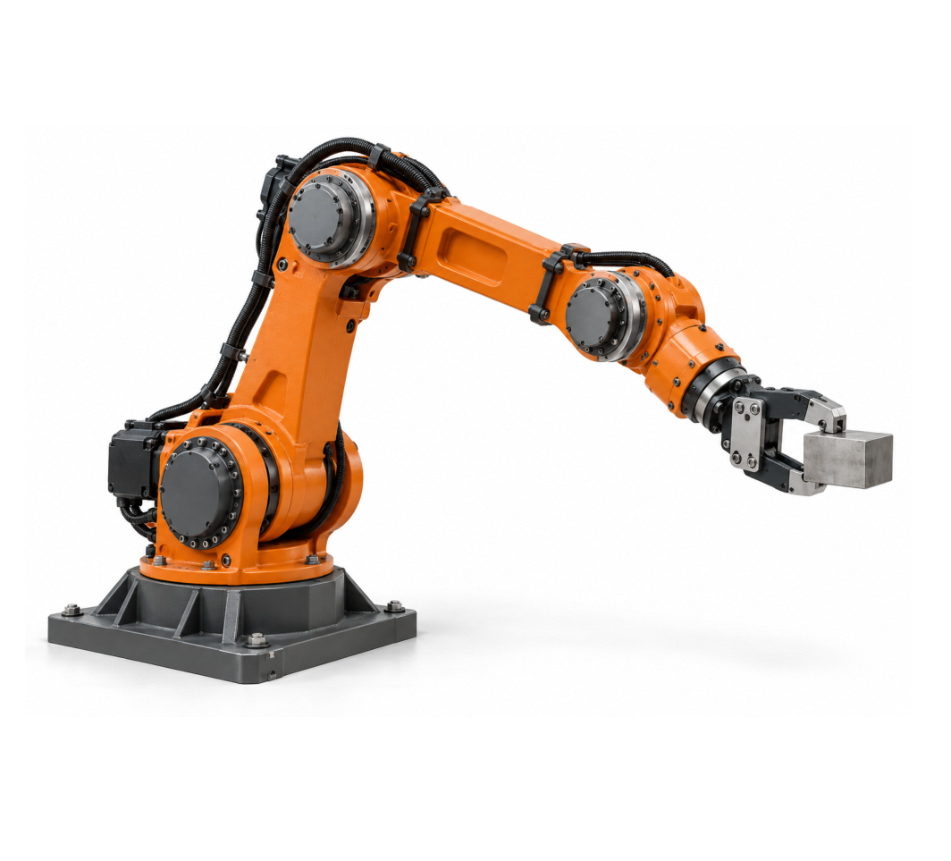
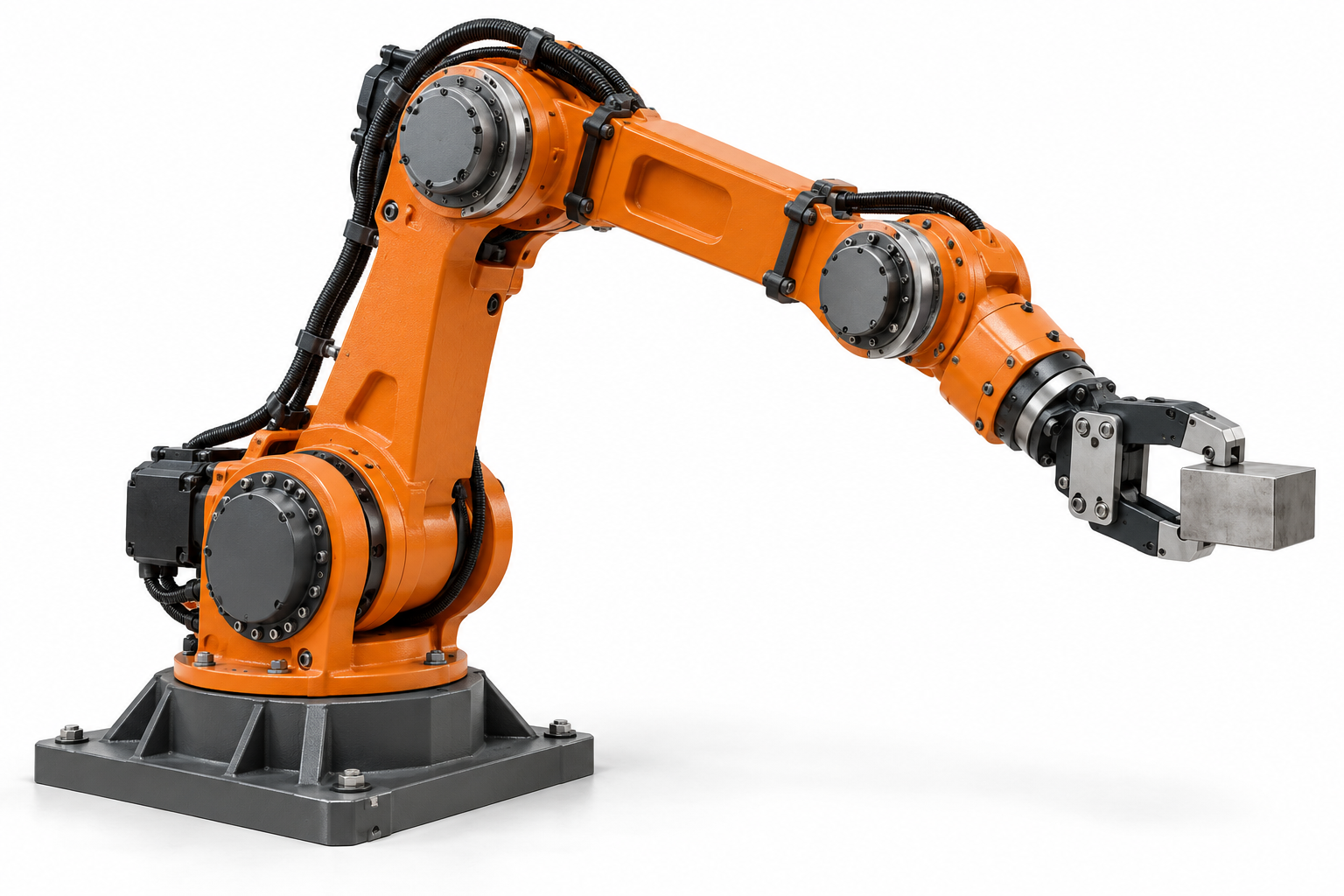
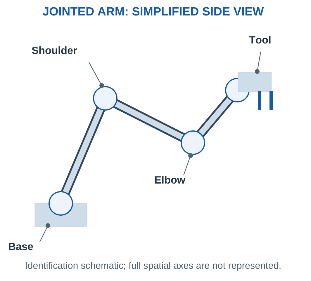
An articulated arm uses serial rotary joints to obtain useful spatial motion.
Many industrial examples have six axes, but the arrangement name does not impose a universal axis count.
Joint limits, link geometry, tool dimensions and loads influence the usable workspace.



Static Joint Moment
For the supplied horizontal model:
Gravity moment = Weight × Perpendicular distance
Tool mass belongs in the load boundary when specified.
A uniform link’s weight acts at its centre under the stated model.
Static gravity moment is not a complete dynamic torque requirement. Acceleration, friction, other links and mechanism effects need additional terms.
Worked Problem 5.51: Payload, Tool and Link
Problem: Payload is 2 kg and tool 0.5 kg at 0.4 m perpendicular arm. A uniform 3 kg link is 0.6 m long. Use g = 9.81 m/s².
Solution:
Payload-plus-tool moment = (2 + 0.5) × 9.81 × 0.4 = 9.81 N m
Link moment = 3 × 9.81 × 0.3 = 8.829 N m
Total = 18.639 N m
Answer: Represented static gravity moment is 18.639 N m.
Worked Problem 5.52: Another Static Boundary
Problem: Payload 1.5 kg and tool 0.4 kg act at 0.3 m. Uniform link mass is 2 kg and length 0.5 m.
Solution:
Load moment = 1.9 × 9.81 × 0.3 = 5.5917 N m
Link moment = 2 × 9.81 × 0.25 = 4.905 N m
Total = 10.4967 N m
Answer: Moment is 10.4967 N m.
Worked Problem 5.53: A Heavier Link
Problem: Payload 3 kg, tool 0.6 kg and arm 0.35 m. Uniform link mass is 4 kg and length 0.7 m.
Solution:
Load moment = 3.6 × 9.81 × 0.35 = 12.3606 N m
Link moment = 4 × 9.81 × 0.35 = 13.734 N m
Total = 26.0946 N m
Answer: Moment is 26.0946 N m.
23. End Effectors and Interfaces to the Task
An end effector is the tool or handling device at the robot’s working end.
Examples include mechanical grippers, vacuum tools and process tools. The interface must transmit the required force and moment and provide any necessary energy, sensing or communication.

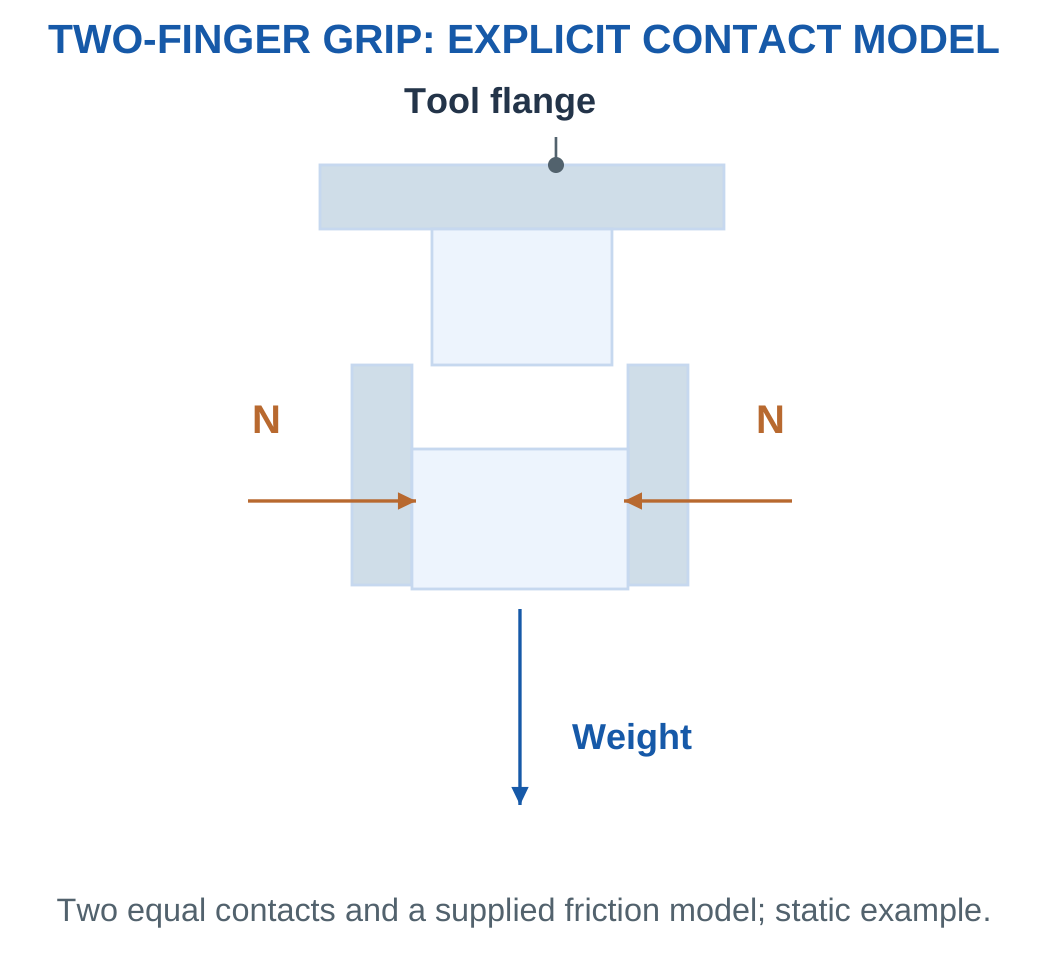
For two equal contacts with normal force N at each contact:
Total ideal friction support = 2μN
If a force is instead supplied as the sum of both contacts, the factor of two must not be applied again.
Vacuum handling uses a different pressure-difference and effective-area model. Actual sealing, leakage, orientation and acceleration matter.
Load Boundary
Tool, adapter and handled object can all contribute to the robot’s moving load.
A payload calculation should follow the stated rating boundary rather than counting only the object.
Worked Problem 5.54: Passing Friction-Grip Screen
Problem: Each of two contacts applies 35 N normal force. Friction coefficient is 0.3 and object mass 1.5 kg.
Solution:
Support = 2 × 0.3 × 35 = 21 N
Weight = 1.5 × 9.81 = 14.715 N
Margin = 21 − 14.715 = 6.285 N
Answer: Ideal support is 21 N, margin 6.285 N, and the supplied static screen passes.
Worked Problem 5.55: Failing Grip Screen
Problem: Each contact applies 25 N, coefficient is 0.25 and object mass 2 kg.
Solution:
Support = 2 × 0.25 × 25 = 12.5 N
Weight = 2 × 9.81 = 19.62 N
Margin = 12.5 − 19.62 = −7.12 N
Answer: The supplied static screen fails.
These simplified results do not independently certify actual handling performance.
24. Workspace, Accuracy, Repeatability and Cycle Time
Workspace describes possible task positions or poses under the stated model.
Actual tools, fixtures, joint limits and surrounding equipment restrict usable access.
Accuracy, repeatability and resolution are different properties.

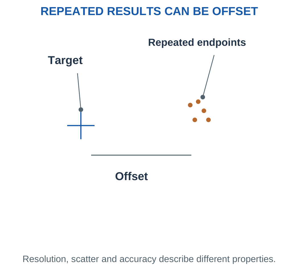
A small command increment does not establish equally small positioning error.
For readings 9.9, 10.0 and 10.1 mm, the mean is 10.0 mm and range 0.2 mm. If the target is 11.0 mm, the mean is still 1.0 mm below target.
Serial Cycle Time
A cycle can include approach, picking, transfer, placement, return and dwell.
When all tasks are serial:
Cycle time = Sum of motion and dwell times
Ideal cycles per minute = 60 / Cycle time
Whole completed cycles require the integer count completed within the stated duration.
Worked Problem 5.56: Cycle Budget
Problem: Motion times are 0.5, 0.8, 0.6 and 0.7 s. Dwells are 0.2 and 0.3 s.
Solution:
Cycle time = 0.5 + 0.8 + 0.6 + 0.7 + 0.2 + 0.3 = 3.1 s
Ideal rate = 60 / 3.1 = 19.3548 cycles/min
Whole completed cycles in 60 s = 19
Answer: Cycle time 3.1 s, rate 19.3548/min, completed count 19.
Worked Problem 5.57: An Exact Count
Problem: Motions are 0.4, 0.6, 0.5 and 0.5 s; dwells 0.25 and 0.25 s.
Solution:
Cycle = 2.5 s
Rate = 60 / 2.5 = 24 cycles/min
Completed cycles in 60 s = 24
Answer: 2.5 s, 24/min, and 24 completed cycles.
Worked Problem 5.58: Two-Minute Output
Problem: Motions are 0.8, 1.0, 0.9 and 0.7 s; dwells 0.3 and 0.3 s.
Solution:
Cycle = 4 s
Rate = 15 cycles/min
Completed cycles in 120 s = 120 / 4 = 30
Answer: 4 s, 15/min, and 30 completed cycles.
25. Drones: Airframe and Subsystem Roles
A drone airframe supports and locates propulsion, battery, control electronics and payload.
In a multirotor, arms and motor mounts maintain the intended rotor relationships while the central structure transfers forces.

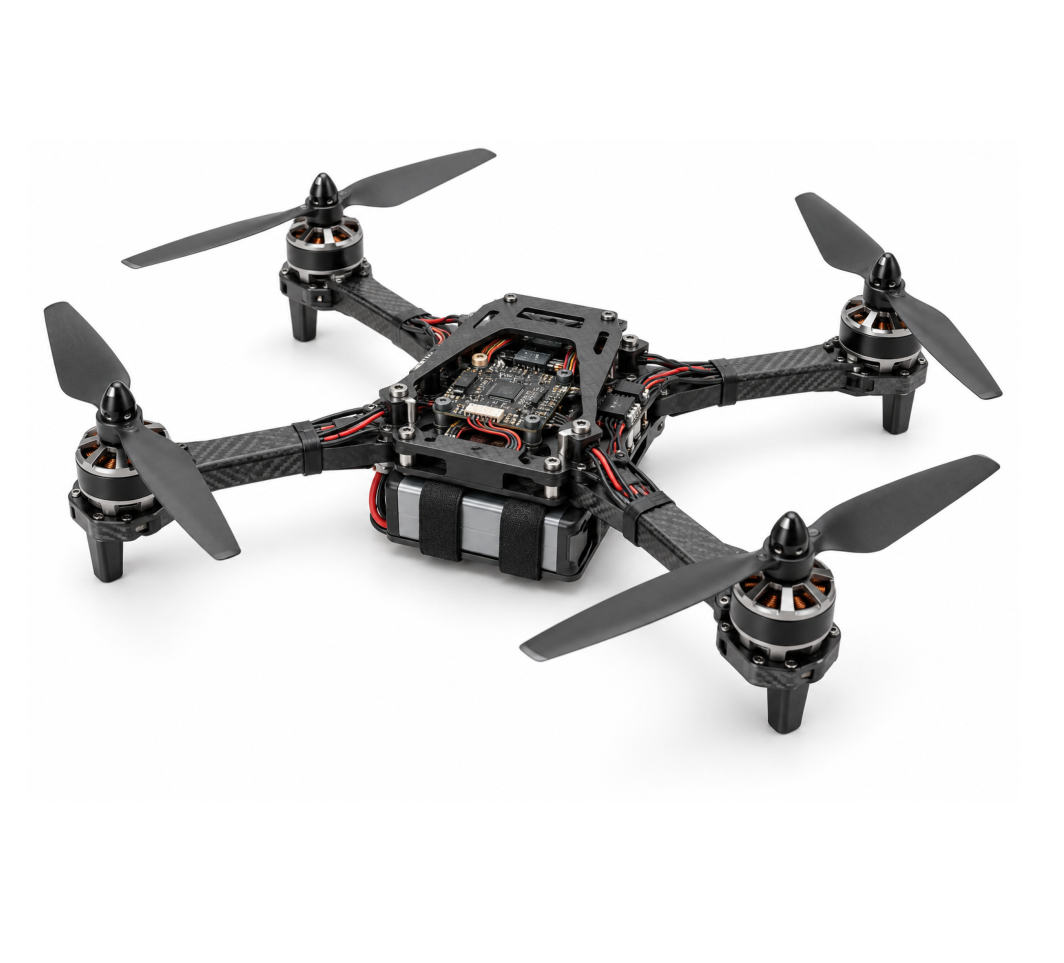

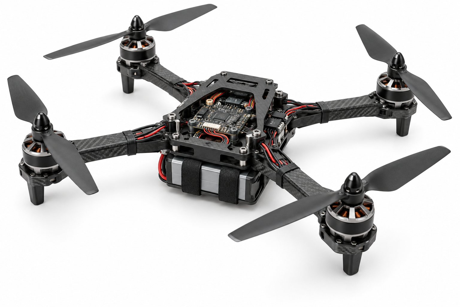


Frame mass, stiffness, mounting and vibration behaviour affect the complete vehicle. A light frame is not automatically suitable.
Payload placement changes total mass and centre of mass.
Subsystem Roles
The battery supplies energy. ESCs switch motor power. Motors and propellers generate propulsion. The flight controller computes commands from references and estimated states.
A communication link carries information rather than all the propulsion energy.
Worked Problem 5.59: Complete Mass Budget
Problem: Frame is 0.25 kg, four propulsion units are 0.06 kg each, battery 0.3 kg, control/wiring 0.1 kg and payload 0.2 kg. Mass limit is 1.2 kg.
Solution:
Total mass = 0.25 + 4 × 0.06 + 0.3 + 0.1 + 0.2 = 1.09 kg
Weight = 1.09 × 9.81 = 10.6929 N
1.09 ≤ 1.2 kg
Answer: Mass is 1.09 kg, weight 10.6929 N, and the screen passes.
Worked Problem 5.60: A Heavier Installed System
Problem: Frame 0.3 kg, four units 0.08 kg each, battery 0.4 kg, control/wiring 0.12 kg and payload 0.3 kg. Limit is 1.4 kg.
Solution:
Mass = 0.3 + 0.32 + 0.4 + 0.12 + 0.3 = 1.44 kg
Weight = 1.44 × 9.81 = 14.1264 N
Answer: Mass is 1.44 kg and the screen fails.
26. Drone Propulsion: Motor, ESC and Propeller
A typical small multirotor uses electric motors and propellers. The propeller interacts with air to generate thrust and resisting aerodynamic torque.
An ESC provides the required motor-power switching according to the intended motor and command interface.

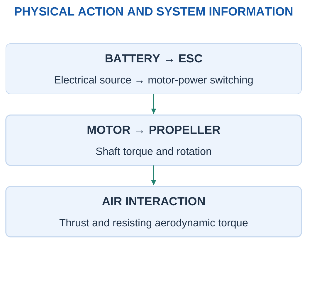
A flight-controller command is not the motor’s high-current energy path.
Many small multirotors use brushless motors, but that statement does not establish a universal pinout or command-to-thrust curve.
Thrust and Power
Thrust is a force. Power is an energy-transfer rate.
A watt value alone does not determine thrust without a propeller/aerodynamic model or relevant data.
Doubling a command does not automatically double rpm, thrust or electrical power.
Energy-Based Duration
For supplied nominal voltage and capacity:
Nominal battery energy = Voltage × Capacity in Ah
The result is in Wh.
Usable energy = Nominal energy × Supplied usable fraction
Ideal duration = Usable energy / Constant total input power
Worked Problem 5.61: Constant-Input Duration
Problem: Four propulsion inputs are 50 W each, with 10 W auxiliary input. Battery is 12 V, 3 Ah and usable fraction 0.8.
Solution:
Total input = 4 × 50 + 10 = 210 W
Nominal current = 210 / 12 = 17.5 A
Nominal energy = 12 × 3 = 36 Wh
Usable energy = 36 × 0.8 = 28.8 Wh
Duration = 28.8 / 210 h = 8.22857 min
Answer: Input is 210 W, nominal current 17.5 A, and model duration 8.22857 min.
Worked Problem 5.62: Another Battery Model
Problem: Four inputs are 70 W each plus 12 W auxiliaries. Battery is 15 V, 4 Ah and usable fraction 0.75.
Solution:
Total = 292 W
Nominal current = 292 / 15 = 19.4667 A
Usable energy = 15 × 4 × 0.75 = 45 Wh
Duration = 45 / 292 × 60 = 9.24658 min
Answer: Model duration is 9.24658 min.
27. Static Hover Force Balance and Simple Margins
For ideal stationary level hover:
Total upward thrust = Weight = mg
For n identical rotors explicitly sharing equally:
Per-rotor thrust = mg / n
Equal sharing depends on the stated model and should not be assumed for every geometry and centre-of-mass condition.

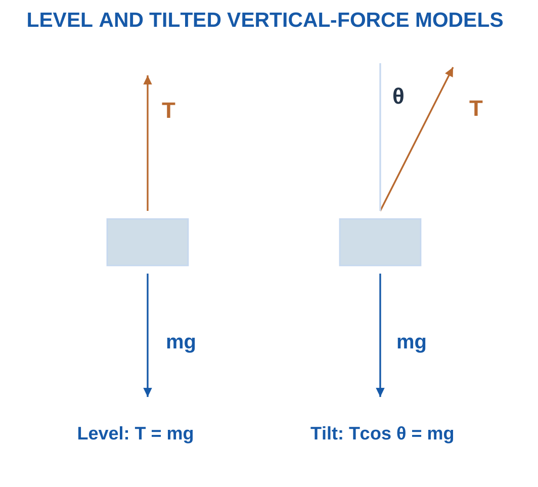
For tilt angle θ from vertical while retaining vertical balance:
T cos θ = mg
Total thrust T = mg / cos θ
Horizontal component = T sin θ
The horizontal component requires a balancing force or implies acceleration. Vertical balance alone is not complete stationary equilibrium.
Worked Problem 5.63: Four-Rotor Model
Problem: Mass is 2 kg, four rotors share equally and each has supplied maximum static thrust 8 N. Also consider 20° tilt.
Solution:
Weight = 2 × 9.81 = 19.62 N
Level share = 19.62 / 4 = 4.905 N/rotor
Maximum total = 32 N
Maximum/weight ratio = 32 / 19.62 = 1.63099
Tilted total = 19.62 / cos 20° = 20.8792 N
Horizontal component = 20.8792 sin 20° = 7.1411 N
Answer: Level share 4.905 N/rotor, ratio 1.63099, tilted thrust 20.8792 N.
Worked Problem 5.64: A 1.5 kg Model
Problem: Four rotors, mass 1.5 kg, maximum 6 N each and tilt 15°.
Solution:
Weight = 14.715 N
Level share = 3.67875 N
Ratio = 24 / 14.715 = 1.63099
Tilted total = 15.2341 N
Horizontal component = 3.94287 N
Answer: Level share is 3.67875 N/rotor.
Worked Problem 5.65: Six Rotors
Problem: Mass 3 kg, six rotors, maximum 7 N each and tilt 25°.
Solution:
Weight = 29.43 N
Level share = 29.43 / 6 = 4.905 N
Ratio = 42 / 29.43 = 1.42712
Tilted total = 29.43 / cos 25° = 32.4724 N
Horizontal component = 13.7234 N
Answer: Level share 4.905 N/rotor, ratio 1.42712, tilted total 32.4724 N.
These static ratios do not independently establish dynamic control capability or endurance.
28. Flight Controller, Sensors and Estimation
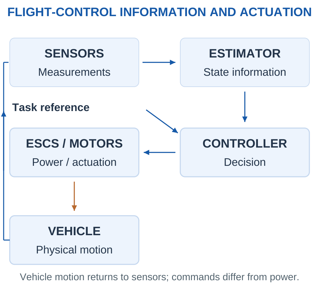
A flight controller uses references and sensor information to estimate relevant states and compute actuator commands.
Control can involve angular rate, attitude and, where provided, position and altitude information.

Sensor Meanings
A gyroscope measures angular rate.
An accelerometer measures specific force. Interpreting its reading as gravity or attitude information requires an appropriate model.
A magnetometer supplies magnetic-field information. A barometer measures pressure. GNSS can provide position and velocity information under its operating conditions.
Sensor fusion combines their different meanings, models and timing. It is not a unit-blind average of all raw readings.
Sampling and Delay
Sample interval = 1 / Sample frequency
Delay can include sensing, computation, communication and actuation effects.
Higher sampling rate alone does not establish stable control or eliminate delay.
Worked Problem 5.66: Sample Interval and Angle
Problem: Sampling is 500 Hz and total delay 6 ms. A constant one-axis gyro rate is 30°/s for 0.1 s.
Solution:
Interval = 1 / 500 = 0.002 s = 2 ms
Delay periods = 6 / 2 = 3
Angle change = 30 × 0.1 = 3°
Answer: Interval 2 ms, delay 3 periods, angle change 3°.
Worked Problem 5.67: A Faster Stream
Problem: Sampling 1000 Hz, delay 4 ms and constant rate 20°/s for 0.2 s.
Solution:
Interval = 1 ms
Delay = 4 sample periods
Angle change = 20 × 0.2 = 4°
Answer: 1 ms, 4 periods, 4°.
Worked Problem 5.68: Negative Angular Rate
Problem: Sampling 200 Hz, delay 10 ms and rate −15°/s for 0.4 s.
Solution:
Interval = 5 ms
Delay periods = 10 / 5 = 2
Angle change = −15 × 0.4 = −6°
Answer: 5 ms, 2 periods, and −6°.
29. Industry 4.0 and Connected Manufacturing
Industry 4.0 describes connected, data-informed manufacturing in which physical processes, sensing, computation, communication and coordinated decisions work together.
It is more than attaching a wireless sensor or displaying a dashboard.

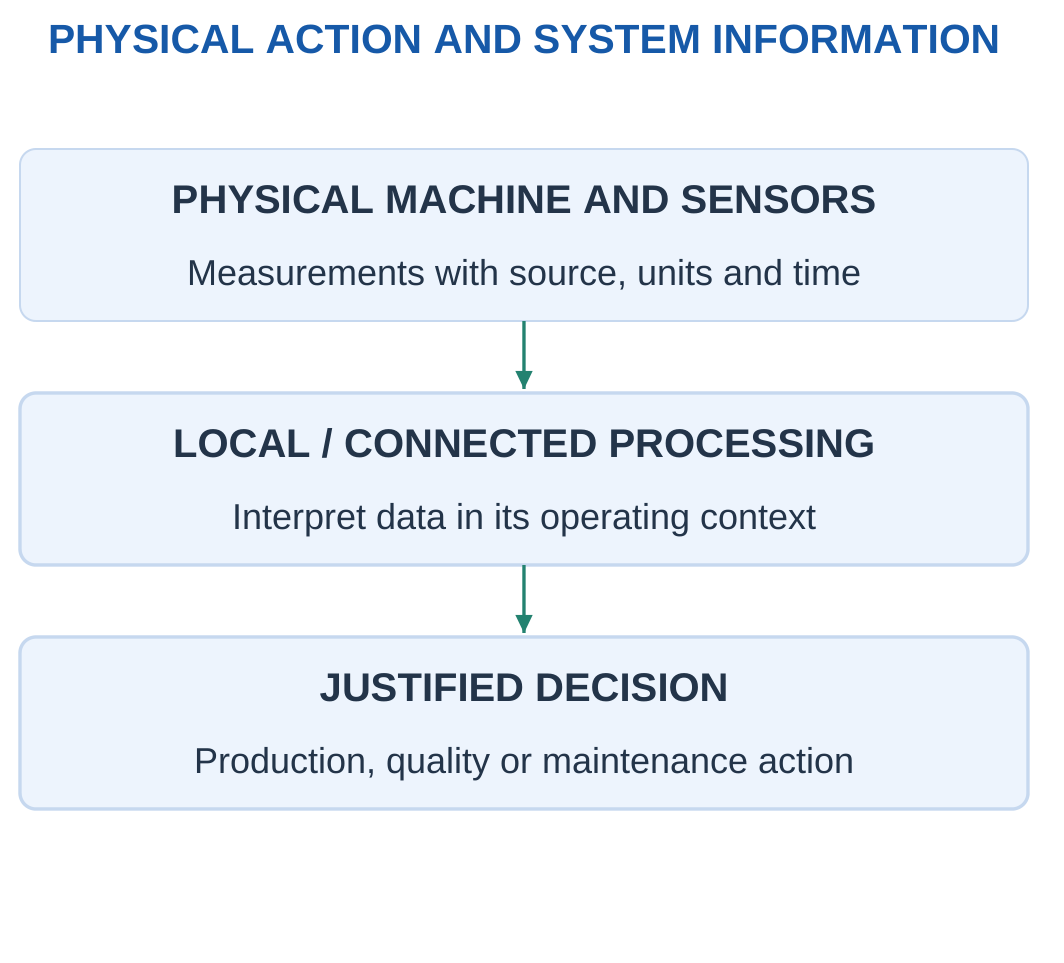
Relevant ideas include industrial connectivity, interoperable data, cyber-physical systems, analytics, digital representations and traceability.
A measurement needs identity, time and units. The system should preserve the connection between the physical source and its digital representation.
Edge and Supervisory Processing
An edge device processes information near the machine. Supervisory or cloud services can support wider analysis.
Location depends on timing, availability, security and the task. An internet path is not automatically suitable for every fast motion loop.
Measuring Improvement
A reduced downtime figure requires a defined baseline and comparable operating conditions.
A dashboard does not prove causation. Data quality and the physical process determine whether the decision is useful.
Worked Problem 5.69: Downtime Reduction
Problem: Scheduled time is 480 min. Downtime changes from 60 to 30 min under comparable operation.
Solution:
Initial available fraction = (480 − 60) / 480 × 100 = 87.5%
Final available fraction = (480 − 30) / 480 × 100 = 93.75%
Relative downtime reduction = (60 − 30) / 60 × 100 = 50%
Answer: Available fractions are 87.5% and 93.75%; downtime reduction is 50%.
The available-time improvement is 6.25 percentage points, which is a different quantity from the 50% downtime reduction.
Worked Problem 5.70: Another Baseline
Problem: Scheduled time is 360 min and downtime changes from 45 to 27 min.
Solution:
Initial fraction = 315 / 360 × 100 = 87.5%
Final fraction = 333 / 360 × 100 = 92.5%
Downtime reduction = 18 / 45 × 100 = 40%
Answer: Fractions are 87.5% and 92.5%, with 40% relative downtime reduction.
30. Condition Monitoring and Maintenance Reasoning
Condition monitoring observes quantities such as vibration, temperature, pressure or current to support assessment of equipment behaviour.
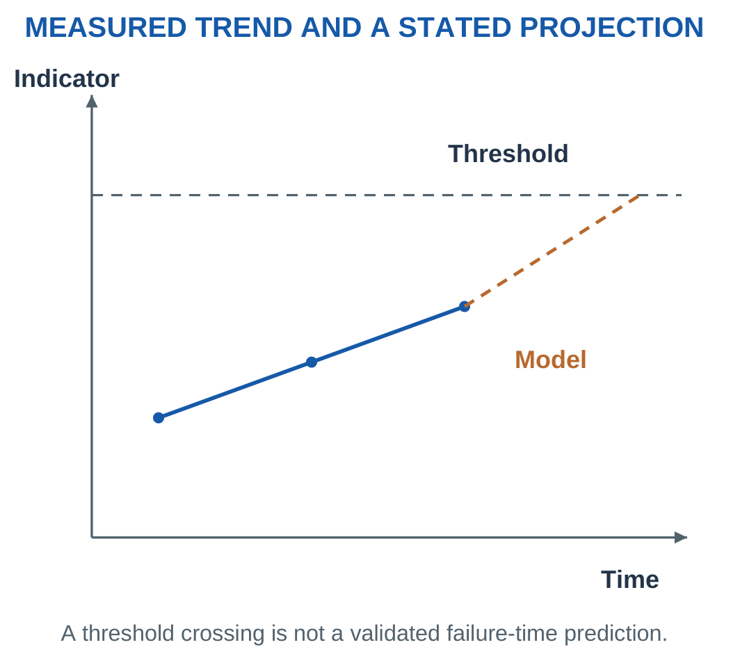
A trend can indicate change, but one threshold crossing does not uniquely identify a fault or establish remaining lifetime.

Maintenance Approaches
Reactive maintenance responds after a fault or event.
Preventive maintenance follows a planned schedule or usage rule.
Predictive approaches use relevant models and evidence to estimate developing condition or future maintenance need.
A threshold alarm alone is not automatically a validated predictive model.
Context
Load, speed, ambient conditions, sensor location and measurement method can affect the reading.
Comparisons should use controlled or understood conditions. Sensor health, timestamp quality and missing data matter before interpreting a trend.
Linear Projection
For a supplied continued linear rise:
Slope = Change in indicator / Change in time
Remaining time = (Threshold − Latest reading) / Slope
The result belongs to that model. Actual progression may be nonlinear or change with operating conditions.
Worked Problem 5.71: Threshold Time
Problem: Indicator is 40 units at 0 min and 46 units at 10 min. Assume continued linear rise. Threshold is 55.
Solution:
Slope = (46 − 40) / 10 = 0.6 units/min
Remaining time = (55 − 46) / 0.6 = 15 min
Answer: Slope is 0.6 units/min and model remaining time is 15 min.
Worked Problem 5.72: A Slower Indicator
Problem: Readings are 2 at 0 min and 2.6 at 15 min. Threshold is 3.5.
Solution:
Slope = 0.6 / 15 = 0.04 units/min
Remaining time = (3.5 − 2.6) / 0.04 = 22.5 min
Answer: 0.04 units/min and 22.5 min.
Worked Problem 5.73: Another Linear Projection
Problem: Readings are 60 at 0 min and 66 at 12 min. Threshold is 75.
Solution:
Slope = 6 / 12 = 0.5 units/min
Remaining time = 9 / 0.5 = 18 min
Answer: Slope is 0.5 units/min and remaining model time 18 min.
31. Data, Digital Twins and System Context
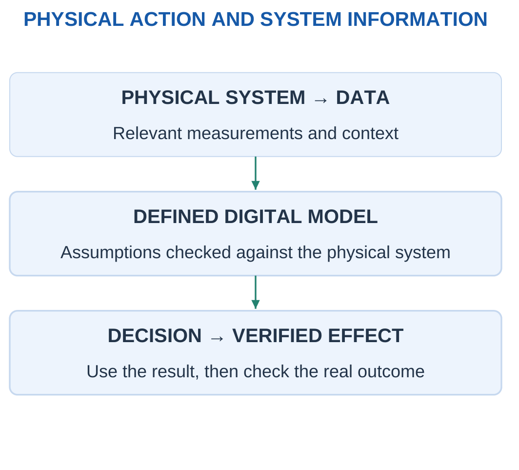
A digital representation can support monitoring, analysis and understanding of a physical system.
A digital twin involves a purposeful connection between the physical system and its digital information or model for a defined use.
A static 3D drawing alone does not establish that ongoing relationship.

Useful Data Context
A data item can require:
- Source identity.
- Timestamp.
- Unit.
- Sensor location.
- Operating mode.
- Quality information.
- Calibration context.
A temperature value without source and time may be unsuitable for comparison.
A model should state its assumptions and be checked against relevant physical observations before its prediction supports a decision.
Data-Volume Arithmetic
Records = Sensors × Records per sensor per second × Duration
Payload bytes = Records × Bytes per record
If overhead is defined as fraction h of payload:
Total bytes = Payload × (1 + h)
Average bit rate = Total bytes × 8 / Duration
The definition of overhead matters. A percentage of payload differs from a percentage of final transmitted total.
Worked Problem 5.74: Six-Sensor Dataset
Problem: Six sensors each produce 100 records/s. Each record has eight payload bytes. Duration is 60 s and overhead is 20% of payload.
Solution:
Records = 6 × 100 × 60 = 36000
Payload = 36000 × 8 = 288000 bytes
Total = 288000 × 1.2 = 345600 bytes
Average bit rate = 345600 × 8 / 60 = 46080 bit/s
Answer: 36000 records, 288000 payload bytes, 345600 total bytes, and 46080 bit/s.
Worked Problem 5.75: Four Sensors at Higher Rate
Problem: Four sensors each produce 250 records/s with 12 payload bytes for 30 s. Overhead is 10% of payload.
Solution:
Records = 4 × 250 × 30 = 30000
Payload = 30000 × 12 = 360000 bytes
Total = 396000 bytes
Bit rate = 396000 × 8 / 30 = 105600 bit/s
Answer: Total is 396000 bytes and average rate 105600 bit/s.
Worked Problem 5.76: Eight-Sensor Dataset
Problem: Eight sensors each produce 50 records/s with 16 payload bytes for 120 s. Overhead is 25% of payload.
Solution:
Records = 8 × 50 × 120 = 48000
Payload = 48000 × 16 = 768000 bytes
Total = 768000 × 1.25 = 960000 bytes
Bit rate = 960000 × 8 / 120 = 64000 bit/s
Answer: 48000 records, 960000 total bytes, and 64000 bit/s.
A large dataset can still contain stale readings, incorrect units or unsuitable measurements. Data quantity is not the same as useful information.
32. Comparison Tables and Formula Sheet
System-Role Comparison
| Element or system | Main role | Important distinction |
|---|---|---|
| Sensor | Measures a physical quantity | Resolution does not automatically establish accuracy |
| Controller | Determines action | Command information is not actuator energy |
| Driver | Interfaces command and power | Must match actuator and supply |
| Stepper axis | Nominal incremental motion | Commands can differ from actual movement |
| Servo axis | Feedback-controlled motion | Sensor location and limits matter |
| Hydraulic actuator | Liquid-powered action | Effective area and opposing pressure matter |
| Pneumatic actuator | Gas-powered action | Compressibility and flow reference matter |
| Cartesian robot | Orthogonal linear-axis motion | Geometric box is not complete usable workspace |
| SCARA | Planar rotary links with additional axes | Relative-angle definitions matter |
| Articulated robot | Serial rotary-joint motion | Axis count and payload depend on design |
| Flight controller | State estimation and command calculation | ESCs deliver motor power |
| Industry 4.0 | Connected physical and digital decisions | Connectivity alone does not prove improvement |
Electric-Actuator Comparison
| Feature | DC motor model | Stepper arrangement | Servo arrangement |
|---|---|---|---|
| Basic description | Electromechanical rotary conversion | Nominal incremental rotor action | Feedback-based motion control |
| Typical arithmetic | Voltage, current, torque and power | Steps, commands, frequency and travel | Reference, measurement and error |
| Feedback assumption | Must be stated | Open-loop use is common but not universal | Feedback is part of the represented arrangement |
| Main caution | Voltage alone does not specify output | Fine commands do not guarantee equal accuracy | Feedback does not remove every mechanical error |
Robot-Arrangement Comparison
| Arrangement | Main geometry | Introductory model |
|---|---|---|
| Cartesian | Orthogonal prismatic axes | Independent travel-box screen |
| SCARA | Planar rotary links plus suitable other axes | Two-link top-view geometry |
| Articulated | Serial rotary joints | Jointed spatial motion and named load moments |
Control and Sensor Relations
Error = Reference − Measurement
Proportional command = K × Error
Physical quantity = (Sensor output − Offset) / Sensitivity
Sample interval = 1 / Sample rate
Constant one-axis angle change = Angular rate × Time
Use the supplied sign convention, limits and measurement definitions.
Motor Relations
Electrical input = VI
Back EMF = V − IR
Electromagnetic torque = ktI
Copper loss = I²R
Converted electromagnetic power = EI
Angular speed = 2πN / 60
Shaft power = Tω
Linear power = Fv
Efficiency = Useful output / Input
Loss rate = Input − Useful output
Stepper Relations
Full steps per revolution = 360 / Full-step angle
Commands per revolution = Full steps × Subdivisions
Nominal command angle = 360 / Commands per revolution
Motor rpm = 60 × Command frequency / Commands per revolution
Direct-screw travel per command = Lead / Commands per revolution
Commands for travel = Travel × Commands per revolution / Lead
Constant-rate time = Command count / Command frequency
Encoder Relations
Angular spacing = 360 / Interpreted counts per revolution
Relative angle = Count change × Angular spacing
Average rpm = 60 × Count change / (Counts per revolution × Interval)
Counts, decoding, direction and wrap assumptions must be supplied consistently.
Hydraulic and Pneumatic Relations
Cap area = πD² / 4
Annular area = π(D² − d²) / 4
Extension pressure force = pcapAcap − prodAann
Available force = Pressure force − Stated opposing forces
Speed = Local chamber flow / Effective area
Stroke time = Stroke × Effective area / Flow
Fluid power = Pressure rise × Flow
1 bar = 0.1 MPa
1 MPa = 1 N/mm²
A standard-condition gas flow is not automatically a local chamber flow.
Robot Relations
Two-link x = L1 cos θ1 + L2 cos(θ1 + θ2)
Two-link y = L1 sin θ1 + L2 sin(θ1 + θ2)
Ideal radial range = |L1 − L2| to L1 + L2
Static moment = Weight × Perpendicular arm
Two-contact ideal friction support = 2μN
Serial cycle time = Sum of stated motion and dwell times
Ideal cycles/min = 60 / Cycle time
Drone Relations
Weight = mg
Level-hover total thrust = mg
Equal rotor share = mg / Rotor count
Tilted vertical balance = T cos θ = mg
Horizontal thrust component = T sin θ
Nominal battery energy in Wh = Voltage × Ah
Ideal constant-input duration = Usable energy / Input power
Data and Monitoring Relations
Trend slope = Indicator change / Time change
Model remaining time = Remaining indicator margin / Trend slope
Payload bytes = Record count × Payload bytes per record
Total bytes = Payload × (1 + Stated overhead fraction)
Bits = Bytes × 8
Average bit rate = Total bits / Duration
33. Short Questions with Clear Answers
1. What Makes a System Mechatronic?
Mechanical action, actuation, sensing, electronics and control are integrated to perform a task.
The explanation must show their interactions. A disconnected parts list or a motor alone does not establish system integration.
2. What Is the Difference Between a Controller and Driver?
The controller determines a command using the task and available information.
The driver interfaces that command with actuator power. Their signal connection does not supply all the load energy.
3. Why Is Feedback Useful?
Feedback reports a relevant output so the controller can compare it with the reference and adjust action.
Its usefulness depends on suitable sensing, mechanics, timing and control. It does not independently guarantee perfect motion.
4. Is Every Stepper System Open Loop?
No. Open-loop stepping is common, but suitable closed-loop stepper arrangements exist.
Open-loop and closed-loop describe the represented control arrangement rather than an absolute motor category.
5. Does Microstepping Guarantee Equal Physical Accuracy?
No. Microstepping provides finer command increments through the driver’s phase-current arrangement.
Actual position depends on motor behaviour, load, driver, mechanics and measurement.
6. What Does Servo Mean?
A servo is a feedback-based controlled-motion arrangement.
Different systems can use different motor technologies, sensors, mechanisms and command interfaces.
7. Does an Encoder Directly Measure Tool Accuracy?
Not necessarily. It measures at its installed location under the stated interpretation.
Backlash, compliance, calibration and attachment can separate a motor-shaft measurement from remote tool position.
8. Why Is Retraction Area Smaller in a Single-Rod Cylinder?
The rod occupies part of the piston section.
The rod-side annular area is the full bore area minus rod area, so the ideal force differs at equal pressure and zero opposing reference.
9. Why Is Air-Flow Reference Important?
Gas volume changes with pressure and temperature.
Standard-condition flow cannot automatically be substituted for local pressurised chamber volume flow in Q/A.
10. How Do Revolute and Prismatic Joints Differ?
A revolute joint permits rotation about an axis.
A prismatic joint permits translation along an axis. Independent coordinates, rather than every visible part, determine degrees of freedom.
11. What Distinguishes Cartesian, SCARA and Articulated Robots?
Cartesian arrangements use orthogonal linear directions.
A common SCARA uses planar rotary links with vertical and tool axes. An articulated arm uses serial rotary joints.
Actual limits and axis counts depend on the design.
12. Is Payload Only the Handled Object?
The rating boundary can include tool, adapter and object.
Tool mass is not automatically free. Use the actual supplied definition.
13. What Balances Weight in Ideal Level Hover?
Total upward thrust equals mg when other vertical effects are neglected.
Equal per-rotor sharing additionally requires an explicit symmetric model.
14. What Do a Gyroscope and Accelerometer Measure?
A gyroscope measures angular rate.
An accelerometer measures specific force. State estimation requires an appropriate interpretation and available supporting information.
15. Is a Threshold Alarm Automatically Predictive Maintenance?
No. A threshold flags a supplied condition.
A predictive claim needs a suitable validated model and context. The crossing alone does not establish cause or remaining lifetime.
34. Complete Examination Answers
1. Explain a Mechatronic System Through a Positioning Axis
A positioning axis integrates a guide, moving carriage, actuator, transmission, power driver, commands and relevant measurement.
The guide constrains motion. A screw or belt converts rotary action into translation. The actuator supplies the required force through that mechanism.
The controller determines the requested action. The driver controls power delivery from the energy source to the actuator.
Signal and power paths must be distinguished. A command carries information while the separate supply provides energy.
A sensor returns information about the physical quantity at its installed location. In a closed-loop model, the controller compares the measurement with the reference and uses the resulting error to influence subsequent action.
An open-loop command-count model does not continuously use measured position to correct the represented output.
A complete diagram should therefore show reference, controller, driver, actuator, mechanism, load and measurement path.
Feedback does not independently remove sensor error, backlash, compliance, delay or saturation. A shaft sensor may report correct motor position while the carriage or tool still differs because of the intervening mechanics.
The task, required accuracy, force, speed, travel and duty determine whether the integrated arrangement is suitable.
2. Compare DC, Stepper and Servo Actuation
A DC motor converts electrical input into rotary mechanical action.
A simplified brushed armature model can use V = E + IR. A supplied torque constant gives T = ktI. Shaft power requires torque and angular speed at the same boundary.
A stepper uses sequenced phase excitation to provide nominal increments. A 1.8° full-step motor has 200 full steps per revolution. At 16 command subdivisions per full step, the nominal command basis is 3200 increments per revolution.
Finer command spacing is not proof of equal physical accuracy. An overloaded open-loop stepper can miss motion without continuous output-position correction.
A servo system uses feedback to control a relevant motion quantity. It includes reference, measurement, controller, driver and actuator or mechanism.
Servo systems can use different motor technologies and sensor locations. A servo is therefore not defined by one universal motor construction or angular range.
Closed-loop stepper arrangements also exist. Motor labels should not be treated as absolute open-loop or closed-loop categories.
Selection requires torque, speed, travel, duty, feedback, driver and mechanism compatibility. Complete-system requirements should be checked before comparing secondary objectives such as cost or mass.
3. Explain Cylinder Force, Direction and Flow Relationships
For bore diameter D and rod diameter d, the full cap-end area is πD²/4.
The rod-side annular area is π(D² − d²)/4.
With extension positive, the pressure-force model is cap pressure multiplied by full area minus rod-side pressure multiplied by annular area.
Known resisting friction or spring forces are applied in the stated direction.
Equal pressure against zero opposing gauge reference produces a larger ideal extension force than retraction because the full area exceeds the annular area.
For a supplied local steady incompressible model, speed is flow divided by effective area. Swept volume is effective area multiplied by stroke, and stroke time is swept volume divided by flow.
The chamber must be identified. Cap-end extension and rod-end retraction use different areas.
Under a matching one-sided ideal model, force multiplied by speed equals pressure multiplied by flow. This checks the power calculation independently.
Hydraulic liquid is often treated as approximately incompressible in the introductory model. Pneumatic compressibility affects stiffness and flow interpretation.
Standard-condition air volume cannot automatically be used as local chamber volume.
Leakage, line losses, dynamics and complete circuit functions require additional information. Pressure-area arithmetic alone does not define the complete operating arrangement.
4. Explain the Three Required Robot Arrangements
A Cartesian robot model uses orthogonal prismatic axes for X, Y and Z positioning.
Its ideal independent-travel region is a rectangular box. Actual fixtures, tools, orientation requirements and surroundings can reduce usable access.
A common SCARA has two rotary planar joints with additional vertical and tool-axis motion.
For a two-link top-view model, the second relative angle adds to the first joint angle when evaluating the second link’s global direction.
Ignoring joint limits and collisions, radial reach lies between the absolute link-length difference and the link-length sum.
An articulated arm uses serial rotary joints. Many industrial examples have six axes, but the arrangement does not impose one universal count.
It provides useful position and orientation flexibility subject to link geometry, joint limits and loads.
Motors, reductions, bearings and housings serve different functions and should not all be counted as independent coordinates.
A robot’s geometric label does not independently establish payload, cycle time, accuracy or collision-free workspace.
The arrangement should be selected against the actual task rather than a general claim that one type is always superior.
5. Explain Encoder Resolution and Why It Differs from Accuracy
If C interpreted counts correspond to one shaft revolution, nominal angular spacing is 360/C degrees.
A count change over a known interval can estimate relative angle and average speed under the stated direction and wrap assumptions.
Quadrature decoding can change interpreted counts per cycle. The specification must identify whether the supplied counts already include decoding.
Resolution describes represented increments. Accuracy describes agreement with the relevant physical reference.
A high-resolution reading can still contain offset, calibration error, attachment slip or reference ambiguity.
An encoder at the motor shaft also cannot directly observe every tool displacement introduced by backlash or elasticity beyond its location.
For 4096 interpreted counts per revolution:
Nominal spacing = 360 / 4096 ≈ 0.08789°
This is not proof that a remote tool has 0.08789° accuracy.
A complete interpretation states sensor location, count definition, mechanical relation and measurement conditions.
The nominal count basis and measured final error should remain separate quantities rather than being treated as interchangeable descriptions of performance.
6. Explain a Drone as an Integrated Mechatronic System
The airframe supports motors, electronics, battery and payload and transfers their forces.
Motors and propellers form the propulsion system. ESCs provide the required motor-power switching. The battery supplies energy.
The flight controller uses task references and interpreted sensor information to compute commands.
A communication link carries information rather than all the propulsion energy.
A gyroscope measures angular rate and an accelerometer measures specific force. Magnetometer, pressure and GNSS measurements can support relevant estimates when provided.
Sensor fusion combines their physical meanings with appropriate models and timing. It is not a unit-blind average of raw signals.
In ideal level hover, total thrust equals mg. Equal rotor sharing requires the explicit symmetry assumption.
Oppositely rotating rotor groups can balance reaction torques in a suitable arrangement. Differential thrust contributes to attitude behaviour, but exact numbering and mixing conventions are vehicle-specific.
Mass, centre of mass, stiffness and mounting also affect the system.
The conceptual explanation connects mechanical structure, power conversion, sensing and control. It does not independently establish complete flight performance from one mass or thrust value.
7. Explain a Level-Hover Calculation and Its Limits
For a supplied 2 kg vehicle and g = 9.81 m/s²:
Weight = 2 × 9.81 = 19.62 N
With four identical rotors explicitly sharing equally:
Per-rotor thrust = 19.62 / 4 = 4.905 N
If each rotor has supplied maximum static thrust 8 N:
Total maximum = 32 N
Maximum/weight ratio = 32 / 19.62 = 1.631
This is a static force ratio rather than a complete payload or control-capability statement.
If total thrust tilts 20° from vertical while retaining vertical balance:
T = 19.62 / cos 20° ≈ 20.88 N
A horizontal component also exists:
Horizontal component = T sin 20°
Without another balancing horizontal force, that component implies horizontal acceleration rather than complete stationary equilibrium.
The model neglects changing aerodynamics, disturbances, thermal limits and transient response.
Thrust is force. Endurance requires energy and power information.
A sufficient static thrust number therefore does not independently establish the full performance of a real vehicle.
8. Explain Industry 4.0 with a Condition-Monitoring Example
A connected manufacturing system can collect vibration, temperature or current together with source identity, timestamp, units and operating context.
Local processing can filter or summarise readings. A supervisory system can support broader interpretation and maintenance or production decisions.
The useful link is between physical operation and a justified decision rather than simply network availability.
Condition monitoring compares measurements under controlled or understood conditions. A rise may indicate change, but load, speed, environment and sensor location can also affect it.
Reactive maintenance responds to an event. Preventive maintenance follows a schedule or usage rule. Predictive maintenance requires a suitable model and evidence about developing condition or future need.
A threshold alarm alone does not prove a future failure time.
A digital twin can support analysis when its representation remains purposefully connected with the physical system. It needs assumptions, current data and validation relevant to its intended use.
A static image or dashboard does not automatically provide these properties.
Improvement claims should use comparable production conditions and a clear baseline. Reduced downtime must be interpreted with the correct denominator.
9. Compare Sample Rate, Data Volume and Useful Information
A uniform sample rate fs gives sample interval 1/fs.
If one fixed-size record is produced per sample and the exercise defines count as rate multiplied by duration, payload storage is record count multiplied by bytes per record.
Separate headers, metadata, compression and endpoint conventions should be included only as specified.
Bits and bytes differ by a factor of eight.
For 1000 records/s, 12 bytes/record and 60 s:
Records = 1000 × 60 = 60000
Payload = 60000 × 12 = 720000 bytes
This number does not establish that the data are accurate, timely or adequate for the physical phenomenon.
Stale timestamps, incorrect units or sensor errors can make a large dataset misleading.
Higher sampling rate also does not automatically remove communication or computation delay.
The task should determine data quantity and timing. Measurement meaning and the complete information path must then be checked.
Storage arithmetic is useful for planning, but it should not be confused with proof of control quality or predictive accuracy.
10. Build a Requirement Screen for an Actuator and Tool
Begin by defining motion type, force or torque, speed, travel, duty and available supply.
Include the tool, adapter and handled payload in the stated mass boundary. Add any required feedback and measurement conditions.
Compare every candidate against every mandatory limit using matching definitions.
A peak rating must not silently satisfy a continuous requirement.
If the task needs 100 N over 80 mm at 50 mm/s, a candidate limited to 60 mm stroke fails even if it provides 200 N.
A lighter or cheaper candidate cannot compensate for missing mandatory travel unless the task explicitly permits such a trade-off.
Only passing candidates should be ranked by the stated secondary objective.
The complete system includes mechanism ratio, sensor location, driver, supply and mounting.
For fluid systems, the pressure source, valve, return or exhaust arrangement and flow conditions belong to the represented system.
Passing the introductory numerical screen establishes the stated feasibility result. Dynamic, thermal, reliability and installation requirements remain additional questions.
11. Explain an Integrated Linear Positioning Calculation
Consider an ideal direct-screw axis with lead 5 mm/revolution, command basis 2000 increments/revolution and constant command frequency 4000 increments/s.
Assume every command is followed, the mechanism has no backlash or slip and acceleration is excluded.
First calculate represented travel per command:
Travel per command = 5 / 2000 = 0.0025 mm
For a 75 mm move:
Command count = 75 / 0.0025 = 30000
Motor speed is:
4000 / 2000 = 2 revolutions/s
Motor speed = 120 rpm
Carriage speed is:
2 × 5 = 10 mm/s
Move time is:
30000 / 4000 = 7.5 s
The independent check is:
75 / 10 = 7.5 s
If a separate measurement reports 74.8 mm at the end:
Reference-minus-measurement error = 75 − 74.8 = 0.2 mm
Nominal command spacing and observed error describe different quantities.
Dividing the error by command spacing does not independently diagnose missed motion, sensor offset, compliance or another cause.
The measured location and model must be stated before interpreting the discrepancy.
35. Integrated Revision and Common Calculation Errors
Separate Commands from Measurements
A command count describes requested motion under a defined command scale.
An encoder count describes sensed information at a particular location.
Actual tool position includes the effects of the intervening mechanics.
These quantities can agree under a supplied ideal model, but they are not identical by definition.
Separate Resolution, Accuracy and Repeatability
Resolution is represented spacing.
Accuracy concerns closeness to the relevant reference.
Repeatability concerns closeness among repeated results.
A system can have fine command spacing, tightly clustered readings and a consistent absolute offset at the same time.
Keep Power Boundaries Consistent
VI describes a stated electrical input.
EI describes converted electromagnetic power in the simplified armature model.
Tω describes shaft power at the named shaft.
Fv describes linear mechanical power at the named load.
Comparing unrelated boundaries can produce a misleading efficiency even when the arithmetic is correct.
Convert Rpm Before Calculating Shaft Power
Torque multiplied by rpm is not directly watts.
Use:
ω = 2πN / 60
Then calculate:
P = Tω
Use the Correct Cylinder Area
Full bore area applies to the cap side.
Annular area applies to the rod side.
Opposing pressure must be included when supplied. Ignoring it changes the represented available force.
State the Flow Reference
Hydraulic Q/A models use the specified local flow and effective chamber area.
Pneumatic gas volume depends on pressure and temperature. Standard-condition flow is not automatically chamber-condition flow.
Include the Tool in the Load Boundary
A robot’s moving load can include the end effector, adapter and workpiece.
Ignoring the tool can understate gravity moment and moving mass.
Distinguish Force from Mass
Mass is expressed in kilograms. Weight and thrust are expressed in newtons.
Use mg to convert mass to weight under the supplied gravitational acceleration.
A force already given in newtons is not multiplied by g again.
Distinguish Static Ratios from Complete Performance
A static thrust-to-weight ratio does not establish endurance or dynamic response.
A static joint moment does not include every acceleration and friction term.
A friction-grip pass does not independently establish complete real handling reliability.
Interpret Condition Trends Carefully
A threshold projection belongs to its stated model.
A trend does not uniquely identify a fault, and an alarm is not automatically a validated prediction of remaining life.
Check Data Definitions
Count records using the supplied rate-duration convention.
Apply overhead to the stated base.
Convert bytes to bits by multiplying by eight.
Do not confuse the amount of stored data with the quality or usefulness of information.
36. Examination Answer Method
Start by identifying the physical task and relevant quantity.
For a positioning problem, identify travel and direction. For a motor problem, identify the electrical and mechanical boundaries. For a cylinder problem, identify the chamber and effective area.
Draw the essential components and label information flow separately from energy flow.
State the model before using equations. Examples include constant rate, followed commands, zero opposing pressure, equal rotor sharing, independent coordinates or linear trend.
Use units to choose the correct relationship.
Commands per second divided by commands per revolution gives revolutions per second. Flow divided by area gives speed. Torque multiplied by radians per second gives power.
Perform an independent check where possible.
For a screw axis, compare command-count time with distance divided by linear speed.
For a hydraulic cylinder, compare pressure-flow power with force-speed power.
For motor power, verify that input equals represented output plus loss under the steady boundary.
For data, verify that average bit rate multiplied by duration recovers total transmitted bits.
Finish with the requested interpretation: position, force, power, efficiency, time, feasible choice or pass/fail result.
Keep the conclusion within the model. A calculated command spacing is not automatically measured accuracy, and a calculated force is not automatically a complete system qualification.