
Electronics Unit 5: Electronic Systems, Industrial and Biomedical Applications
Subject: Fundamentals of Electronics Engineering
University: AKTU
Course: B.Tech First Year
Semester: I & II
Course Codes: AEC101A / AEC201A | AEC101B / AEC201B | AEC101C / AEC201C
Applicable Streams: CSE, EE, ECE, CE, ME, CH, TX, BT & AG
Unit V Introduction
Electronic systems combine sensing, processing, communication and power to produce useful information or action. This combined unit connects embedded-system fundamentals with industrial automation, biomedical instruments and precision-agriculture applications.
Topics Covered
| Topic | Pages |
|---|---|
| MCU, GPIO and input interfaces | 3–6 |
| ADC types, timing and PWM | 6–14 |
| UART, SPI, I2C and signal chains | 14–19 |
| Wireless and power management | 19–24 |
| A-group embedded applications | 24–27 |
| PLC, VFD, SCADA and IIoT | 27–30 |
| Biomedical instrument concepts | 30–33 |
| Solar, drones, agriculture and revision | 33–37 |
Coverage
All six A/B/C course codes and nine streams. The branch-wise topic guide identifies the prescribed sections. Read the shared foundation, then follow your prescribed application sections.
How to Use These Notes
- Start with the branch/topic guide.
- Trace information and energy as separate paths.
- Identify sensing, conditioning, conversion and control.
- State timing, calibration and power assumptions.
- Distinguish a command from the action achieved.
- Check units, interfaces, bandwidth and energy budget.
What Is Included?
| Study Support | Included |
|---|---|
| Worked problems | 50 numbered problems with steps and checks. |
| Labelled figures | Conversion, communication, power and application paths. |
| Realistic images | 10 component and application photographs. |
| Dedicated applications | Embedded/IoT systems, industrial automation, biomedical and agri electronics. |
| Revision | Formula conditions, memory cues and short answers. |
Key Distinction
A sensor reports a physical condition, a controller makes a decision, a driver switches load power and a communication link carries information. One block does not automatically perform all four roles.
Numerical Convention
Values are educational assumptions. Retain precision until the final answer. An approximate model is valid only within its stated conditions.
Unit Overview and Branch-Wise Reading Map
The three groups have different Unit V application requirements. Follow the dedicated sections below; shared foundation lessons support reading the system diagrams. A-only converter/interface detail is enrichment for B/C unless explicitly needed by an application.
| Topics / Application Block | Applicable Branches | Where to Read |
|---|---|---|
| System blocks, microcontroller and GPIO; signal-chain reading | A prescribed; supporting foundation for B/C | Sections 1–5, 22–23 |
| ADC including digital-ramp/flash, PWM; UART, SPI, I2C | A: CSE, EE, ECE | Sections 6–21 |
| Bluetooth, Wi-Fi, Zigbee; LDO / DC-DC; weather station, home node and BMS | A: CSE, EE, ECE | Sections 24–33, 35 |
| Wearable health-monitor electronics | A: CSE, EE, ECE; C: BT, AG | Section 34; related C instrument sections |
| PLC inputs/outputs/ladder and VFD rectifier/DC bus/inverter | B: CE, ME, CH, TX | Sections 36–37 |
| SCADA/HMI, industrial wireless/IIoT and motor condition monitoring | B: CE, ME, CH, TX | Sections 38–40 |
| ECG, pulse oximeter, glucometer and portable ultrasound | C: BT, AG | Sections 41–44 |
| Solar controller, IoT soil node, drone ESC/BLDC/GPS, irrigation and greenhouse | C: BT, AG | Sections 45–48 |
| Formula conditions and final revision | All: select relevant topics | Section 49 and revision page |
Syllabus Groups and Official Unit Names
- A — CSE, EE, ECE: Electronic Systems and Emerging Applications.
- B — CE, ME, CH, TX: Industrial Electronics and Smart Systems.
- C — BT, AG: Biomedical and Agri Electronics – Emerging Applications.
What Is Included
50 numbered solved problems, 10 realistic component/laboratory images, labelled system illustrations, model checks and revision. Both semester codes within each group use the same unit syllabus. Dedicated [B] and [C] labels identify the additional prescribed application blocks.
Reading rule: Explain each block, trace the measurement or command, identify its power source and state its practical limitation. Numerical examples use declared teaching models rather than universal equipment specifications.
1. Electronic Systems: Sensing to Useful Action
An electronic system combines inputs, processing, outputs, communication and power. A sensor converts a physical quantity into an electrical signal. Conditioning prepares that signal, a converter may digitise it, and a controller interprets the information. An output can be a display, a transmitted message or a controlled actuator.
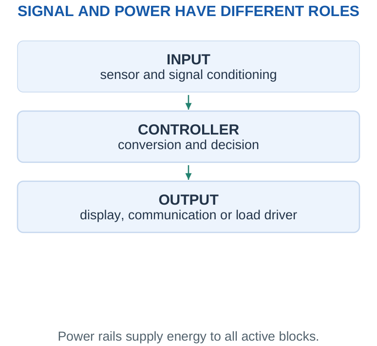
Links with earlier units: Diodes and transistors provide protection and load switching; op-amps amplify and condition signals; logic circuits represent, route and store data. This unit assembles these ideas into complete applications.
Choosing one impressive component does not by itself establish a working system: voltage ranges, timing, references, interfaces and power requirements must agree. A signal carries information; a power path delivers energy. An MCU output can command a motor driver without supplying motor current directly. A wireless link can carry a measured temperature without carrying the sensor’s electrical supply.
Exam approach: When asked to explain a system, name the physical input, sensor, conditioning, conversion, controller, communication/output and supply. Then trace what each stage does to the information.
Worked Problem 5.1: Identify the Energy and Information Paths
Problem: A temperature sensor sends a small voltage to an MCU-controlled fan system. List the signal stages and explain whether the sensor powers the fan.
Model / approach: Separate measurement information from actuator energy.
Step 1: Signal: sensor → conditioning → ADC → MCU decision → compatible fan driver.
Step 2: Energy: the fan supply provides fan current through the driver. The sensor and MCU also need their own valid power rails.
Answer: The sensor controls information; a suitable supply and driver deliver fan energy.
Check and interpretation: A logic command is not a guarantee of load-current capability. A complete physical arrangement must also provide compatible command levels, references and any required inductive recirculation path.
2. What a Microcontroller Contains
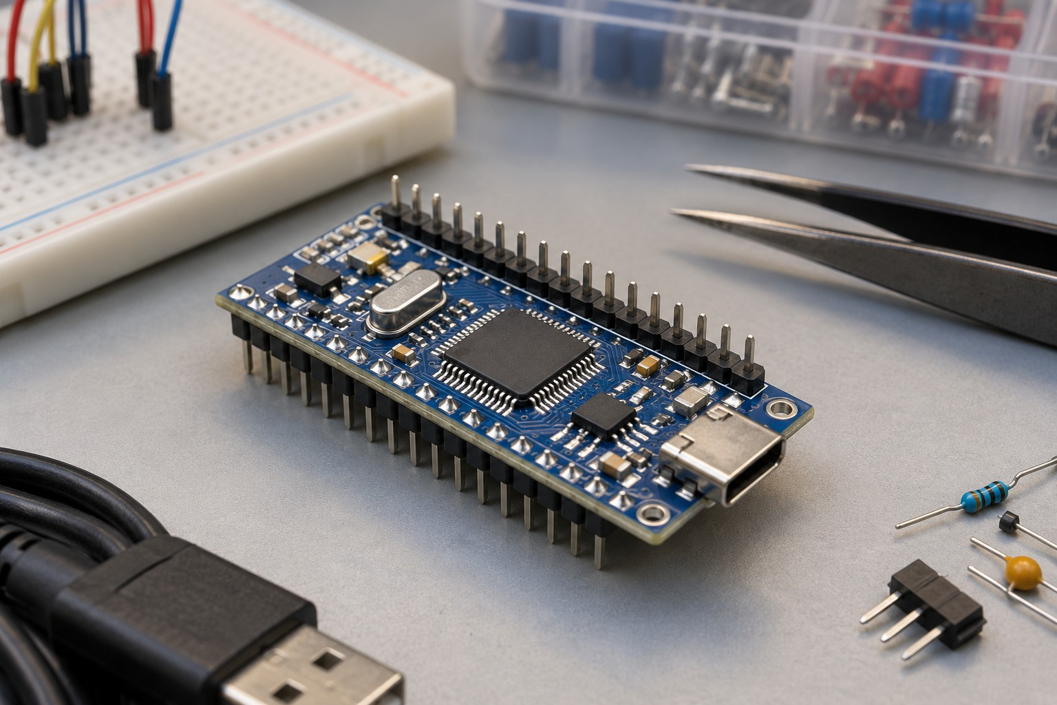
A microcontroller (MCU) integrates a processor core, program memory, working memory and useful peripherals into one device. The processor executes instructions, program memory holds the application, RAM holds temporary data and peripheral hardware handles tasks such as timing, conversion and serial communication.
Worked check: Pin roles are alternatives
A package may list UART TX, PWM output and GPIO on one physical pin as alternate functions. That listing does not create three independent wires. If an application needs simultaneous separate TX and PWM paths, confirm that suitable distinct pin assignments exist. Peripheral names alone do not settle the pin budget.
Worked check: ADC channels versus converters
Eight external ADC input channels do not necessarily mean eight simultaneous conversions. If one converter is multiplexed among them, eight channels at 100 samples/s each require at least 800 conversions/s plus acquisition and scheduling overhead. The hardware architecture determines whether channels share timing.
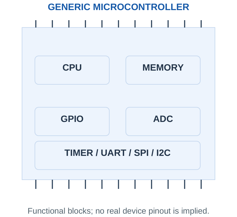
A microprocessor typically depends more heavily on external system components, while an MCU is designed for embedded control. This is a broad architectural distinction, not an absolute rule about speed, cost or every modern chip. A system-on-chip may combine many further functions, including radios or application processors.
An MCU does not necessarily contain every peripheral shown in a textbook. Some have no internal ADC, others integrate several ADC channels, and only selected pins may support a chosen alternate function. Pin count, ADC channel count and number of independent conversion cores are different quantities.
Important distinction: Flash program memory stores instructions; a flash ADC is a parallel conversion architecture. The shared word “flash” does not make them the same hardware block.
3. Clock, Memory and Peripheral Overview
A clock provides timing for instruction execution and peripherals, often through internal dividers. A faster clock gives shorter clock periods but does not imply one complete instruction or one ADC conversion per clock. Different blocks can use different derived clocks and numbers of cycles.
Worked check: Allocated sample size
A two-channel buffer stores 1000 samples per channel at two bytes each. It uses 2 × 1000 × 2 = 4000 bytes before timestamps. If each ADC result has twelve significant bits, storing it in sixteen bits does not change the ADC resolution; it changes the allocated representation.
Worked check: Clock divider estimate
A supplied timer clock is a 16 MHz source divided by 8. Its tick rate is 2 MHz and tick period is 0.5 µs. An interval of 200 ticks is therefore 100 µs. Use the peripheral’s actual derived clock rather than substituting the processor clock without its divider.
| Block | Basic Role |
|---|---|
| CPU | Executes control and arithmetic instructions |
| Program memory | Holds firmware instructions |
| RAM | Holds samples, variables and temporary buffers |
| Timer/counter | Measures intervals, counts events or sets PWM timing |
| ADC | Converts analog input into a numerical code |
| UART, SPI, I2C | Exchange serial information with other devices |
| GPIO | Reads or drives configured digital pins |
A sample buffer consumes memory according to sample count and stored bytes per sample. An ADC with twelve useful bits may still be stored in a two-byte word for convenient alignment. The number of significant bits and allocated storage size should not be confused.
Scope: The syllabus asks for an MCU overview and peripheral concepts. The following calculations use supplied clock, storage and timing models rather than assuming a particular chip or instruction set.
Worked Problem 5.2: Clock Period and Peripheral Interval
Problem: A peripheral uses 40 clocks from a stated 16 MHz clock per event. Find clock period and event interval.
Model / approach: Assume this peripheral directly uses the given clock with no extra divider.
Step 1: Tclk = 1/(16 × 10^6) = 62.5 ns.
Step 2: Tevent = 40Tclk = 2.5 µs.
Answer: Clock period 62.5 ns; event interval 2.5 µs.
Check and interpretation: The event needs the supplied number of clocks. It is not valid to claim every instruction, conversion or serial byte completes in one processor clock.
4. GPIO Input and Output Behaviour
General-purpose input/output (GPIO) pins connect digital signals to the controller. An input senses a voltage using its defined thresholds; an output drives a level within its specified voltage and current limits. Some pins can instead be assigned to analog input or an alternate peripheral function.
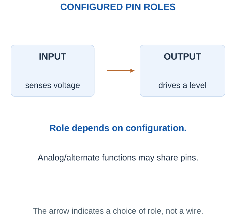
A push-pull output actively drives both HIGH and LOW. An open-drain output actively pulls LOW and otherwise releases the line, so a pull-up or another defined source establishes HIGH. Do not connect two independently driven push-pull outputs together and expect ordinary bus behaviour.
Practical interface checks: Check the pin’s voltage tolerance, the receiver thresholds, output current and common reference. A 3.3 V MCU is not automatically tolerant of a 5 V sensor output. A relay or motor normally requires a compatible driver, not direct connection to a signal pin. Input and output current limits are device-specific and must come from supplied data.
Interpretation: The logical meaning of a bit comes from the application. LOW can mean “pressed”, “alarm active” or “device selected”; it does not always mean the action is OFF.
Worked Problem 5.3: GPIO Voltage-Level Compatibility
Problem: Driver HIGH ≥ 3.0 V and LOW ≤ 0.2 V. Receiver requires HIGH ≥ 2.3 V and LOW ≤ 0.8 V. Find voltage noise margins. Assume other input limits and loading conditions are satisfied.
Model / approach: Compare guaranteed output and input levels.
Step 1: High margin = 3.0 – 2.3 = 0.7 V.
Step 2: Low margin = 0.8 – 0.2 = 0.6 V.
Answer: Voltage-level screen passes.
Check and interpretation: A negative high margin means the receiving input is not guaranteed to recognise the driver HIGH. Merely naming both circuits digital does not make their voltage ranges compatible.
Worked Problem 5.4: Why a Driver Is Required
Problem: A hypothetical GPIO may provide 4 mA at its valid HIGH voltage. A load needs 80 mA. Can the pin directly supply the required load current?
Model / approach: Compare current demand and the stated output capability.
Step 1: Required current = 80 mA; allowed direct output current = 4 mA.
Step 2: The demand is 80/4 = 20 times the stated capability.
Answer: No. Use an appropriate compatible load driver.
Check and interpretation: A correct HIGH voltage with no load does not prove that voltage remains valid under an excessive load. A transistor choice also needs its own drive and load checks.
5. Pull-Ups, Switches and Digital Sensor Inputs
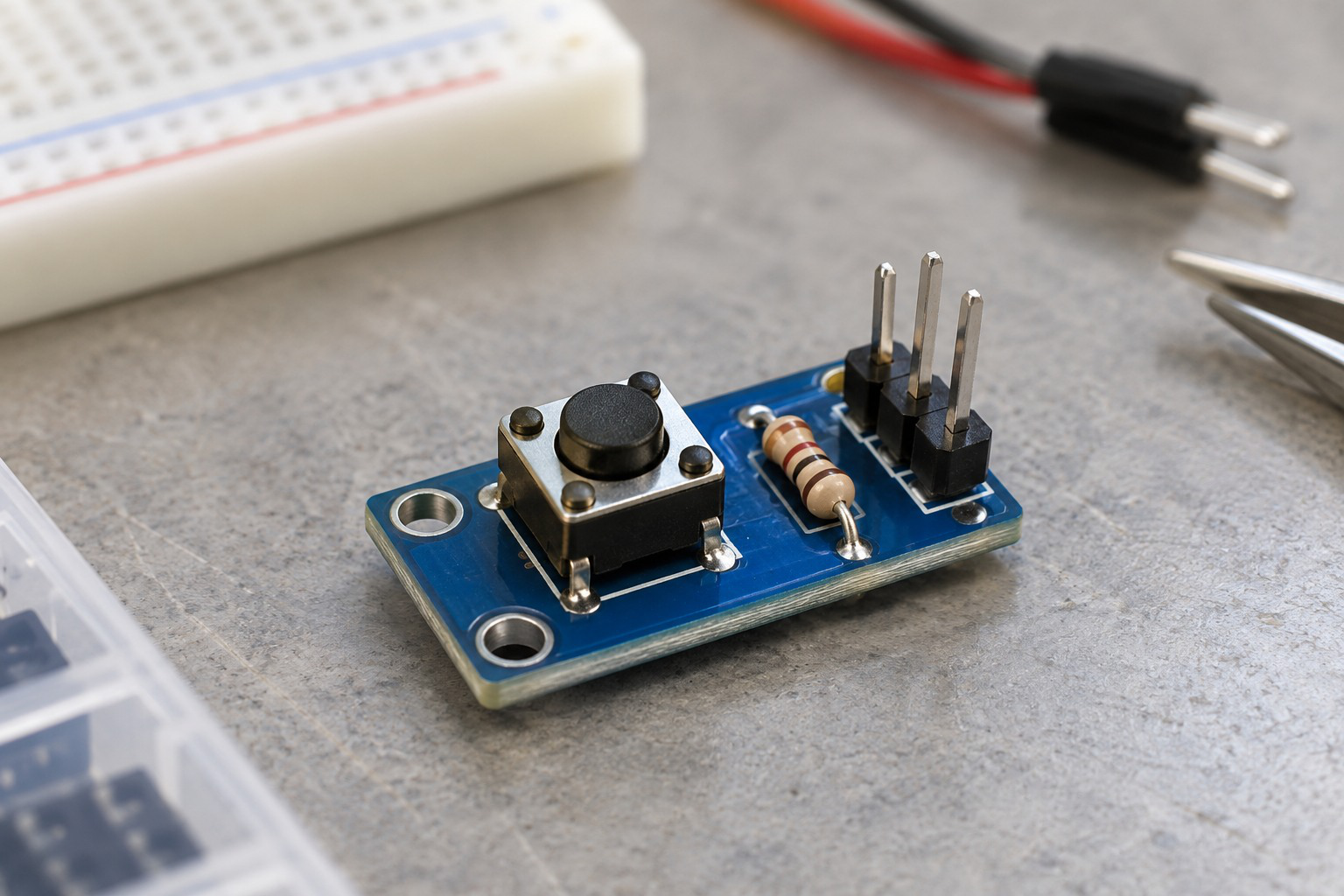
A floating input can respond unpredictably to interference or leakage. A pull-up resistor establishes a default HIGH level when a switch is open. Closing the switch to ground makes the input LOW. This common arrangement gives an active-LOW pressed or contact-closed signal.
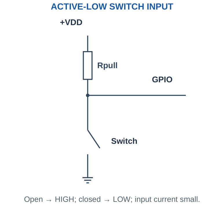
For an ideal closed switch, current is approximately VS/Rpull and resistor power is VS²/Rpull. A small resistor improves resistance to some leakage effects but increases closed-state current. A very large resistor reduces current but may give a weaker default level or slower rise with capacitance.
Mechanical contact bounce produces multiple transitions during one physical action. Debouncing can use hardware or a time-based decision; no program is required to understand the problem. A digital sensor may already provide a clean logic output, but voltage compatibility and output type still matter.
Model condition: The simple current formula assumes the switch clamps the node near ground and the input current is negligible. Leakage and finite switch voltage can change the actual input level.
Worked Problem 5.5: Pull-Up Current and Power
Problem: A pull-up of 4700 Ω connects an input to 5 V. An ideal closed switch grounds the input. Find closed-state current and resistor power; neglect leakage.
Model / approach: The closed switch puts the supply across the resistor.
Step 1: I = 5/4700 = 1.0638 mA.
Step 2: P = V²/R = 5.3191 mW. Open-switch current is negligible in this model.
Answer: Iclosed ≈ 1.0638 mA; P ≈ 5.3191 mW.
Check and interpretation: Open gives a HIGH input and closed gives LOW with compatible thresholds. Changing the pull-up resistance affects current and susceptibility to leakage, not the intended active-LOW interpretation.
6. Analog-to-Digital Conversion
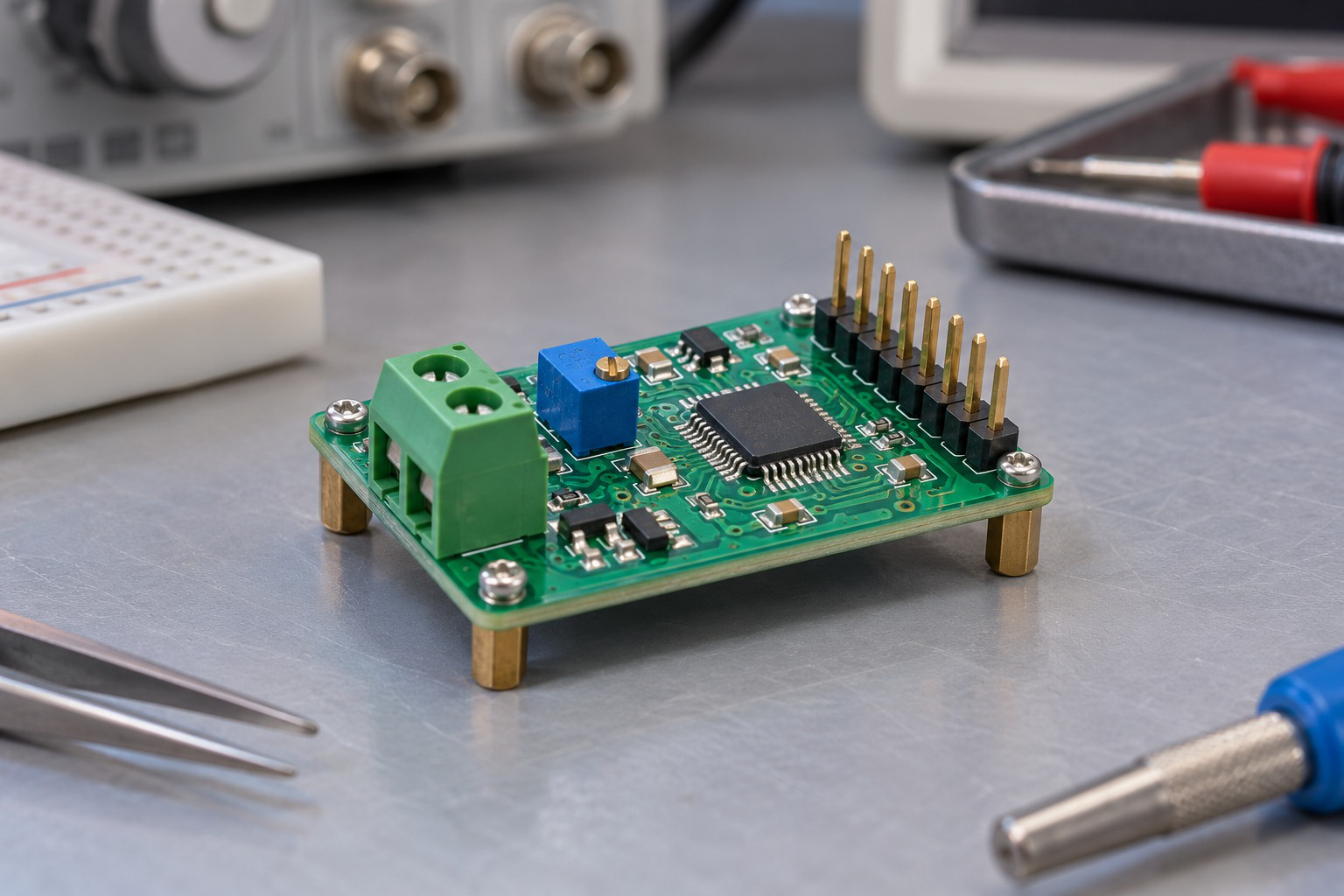
An analog-to-digital converter (ADC) maps an input voltage into a digital code. The code represents an interval of analog values rather than an infinitely precise voltage. The controller can then compare, record or communicate the code.
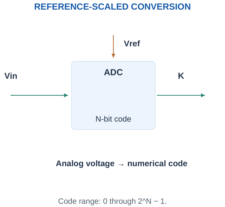
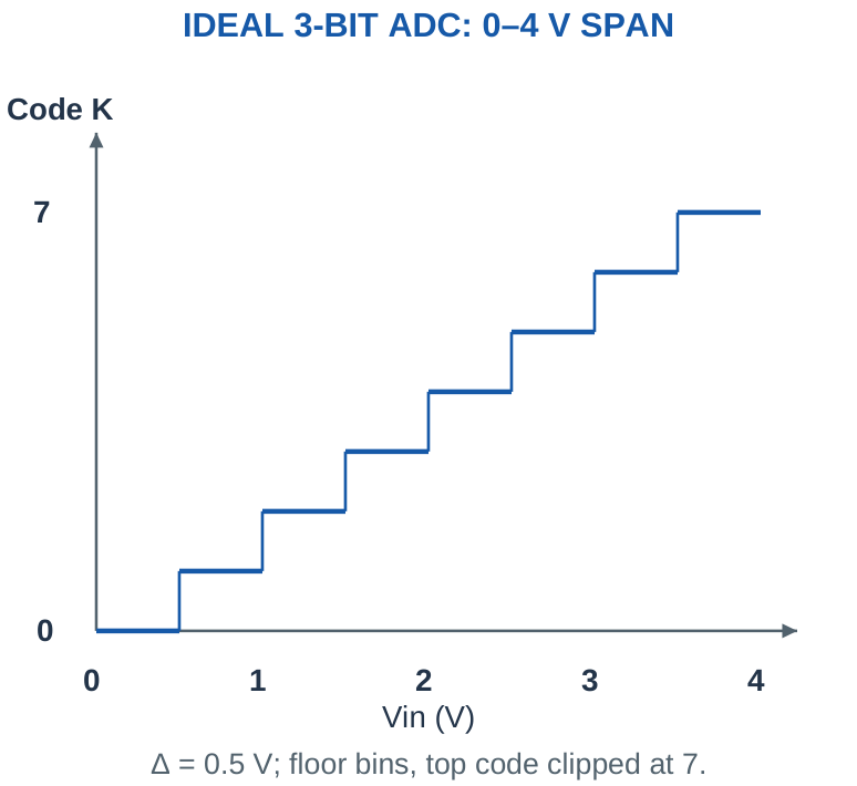
For an ideal N-bit unipolar model spanning 0 to Vref, there are 2^N codes, numbered 0 through 2^N – 1. The nominal bin width is Δ = Vref/2^N. More bits divide the same span into smaller intervals, but do not by themselves remove sensor error, noise, offset or a poor reference.
Stated convention for general code problems: Unless a problem specifies another transfer rule, use K = floor(Vin/Δ) for 0 ≤ Vin < Vref and clip to the valid code range when explicitly considering the endpoints. Code K corresponds to the bin KΔ ≤ Vin < (K + 1)Δ. Device-specific transition rules can differ; the counter-ramp examples state their own first-crossing rule separately.
Distinguish: Resolution is the step size or bit count. Accuracy concerns closeness to the true physical input and includes other errors.
Worked Problem 5.6: Code Count and Nominal Bin Width
Problem: An ideal 8-bit ADC spans 0–5 V. Find code count, largest code and bin width.
Model / approach: Use 2^N bins across the span.
Step 1: Code count = 2^8 = 256. Maximum code = 255.
Step 2: Δ = 5/256 = 19.5312 mV.
Answer: 256 codes; maximum 255; Δ ≈ 19.5312 mV.
Check and interpretation: The maximum code is one less than the code count. The span/bin-width model uses 2^N in its denominator; an endpoint display scale is a separate convention.
7. ADC Resolution and Physical-Unit Sensitivity
With input span Vspan and N bits, an ideal uniform bin width is Vspan/2^N. If the sensor produces S volts per physical unit and conditioning gain is G, the ideal physical increment per code is Δ/(GS), provided the mapping is linear and no stage clips.
A reference of 4.096 V with twelve bits gives a 1 mV nominal bin width. This convenient model value is not a statement that all twelve-bit ADCs use that reference. When comparing two ADC resolutions, keep the same span unless a different span is explicitly given.
A common endpoint scaling formula V ≈ K Vref/(2^N – 1) makes the highest code display Vref. It is a display/calibration convention, not the same definition as the bin width Vref/2^N. Do not switch denominators inside a problem without explaining which model is being used.
Exam habit: Write the selected ADC transfer convention before calculating a code, a reconstructed voltage or a sensor-unit increment.
Worked Problem 5.7: Physical-Unit Increment per Code
Problem: ADC has 12 bits and 4.096 V span. A sensor has sensitivity 10 mV/°C and conditioning gain 4. Find nominal °C per ADC bin. Assume a linear unclipped path.
Model / approach: Divide ADC voltage increment by the amplified sensitivity.
Step 1: Δ = 4.096/4096 = 1 mV.
Step 2: Output sensitivity = 4 × 10 = 40 mV/°C.
Step 3: Increment = Δ/(GS) ≈ 0.025 °C/code.
Answer: Nominal increment ≈ 0.025 °C per bin.
Check and interpretation: This is an ideal increment, not total temperature accuracy. Sensor error, reference variation, offset and noise have not been specified by the bit count.
8. ADC Codes, Intervals and Reconstruction
Under the floor-bin model, the code identifies an interval, not one exact voltage. A lower-edge estimate is KΔ; a midpoint estimate is (K + 0.5)Δ. For an input inside a bin, midpoint reconstruction has quantisation-error magnitude no greater than half a bin in the ideal model.
Worked check: Floor-bin and first-crossing codes
For Vin = 1.234 V and Δ = 0.01 V, a floor-bin ADC gives code 123, while the explicitly defined upper-crossing counter gives 124. Its trial DAC reaches 1.24 V. Both results are consistent with their own stated thresholds; they must not be presented as one unexplained rounding convention.
Worked check: Midpoint versus lower edge
If code 10 has Δ = 0.1 V, its floor-model input interval is 1.0 ≤ Vin < 1.1 V. The lower-edge estimate is 1.0 V and midpoint estimate is 1.05 V. At true input 1.08 V, their estimate-minus-input errors are -80 mV and -30 mV respectively.
Use signs consistently: Define error as estimate minus true input, or the reverse, and state that choice. A floor-code lower-edge estimate has an error from approximately -Δ up to zero for in-range inputs. It should not be assigned a universal ±Δ/2 bound unless midpoint or an appropriate rounding model is used.
At Vin = Vref, the clipped maximum code is 2^N – 1; there is no additional code 2^N. An out-of-range voltage must not be wrapped into a valid low code. Real ADC input limits may be stricter than a purely numerical clipping model.
Decode carefully: Convert a binary code to its unsigned integer before scaling. A ten-bit output code is not automatically the same thing as a ten-bit voltage value written in volts.
Worked Problem 5.8: Code, Bin and Midpoint Estimate
Problem: Use the floor-bin model for an ideal 8-bit 0–4 V ADC with Vin = 1.02 V. Find code, its interval and midpoint estimate.
Model / approach: K = floor(Vin/Δ); estimate = (K + 0.5)Δ.
Step 1: Δ = 0.015625 V; Vin/Δ = 65.28, so K = 65 (binary 01000001).
Step 2: Input interval: 1.015625 ≤ Vin < 1.03125 V.
Step 3: Midpoint estimate = 1.0234 V; estimate – Vin = 3.4375 mV.
Answer: K = 65; midpoint estimate 1.0234 V.
Check and interpretation: The true input lies inside the stated bin, and midpoint error is within half a bin. A lower-edge estimate would have a different signed error; it should not silently inherit midpoint rounding assumptions.
Worked Problem 5.9: Upper Endpoint and Clipping
Problem: An ideal 8-bit ADC spans 0–4 V. Under a stated numerical clipping rule, find the code for Vin = 4 V and explain why code 256 is invalid.
Model / approach: The valid codes run from 0 through 255.
Step 1: The unbounded ratio is 4/(4/256) = 256.
Step 2: Apply the specified maximum-code clipping: K = 255 = 11111111.
Answer: The clipped code is 255.
Check and interpretation: No nine-bit code 256 exists in the eight-bit output. This is a numerical endpoint convention, not permission to exceed the actual analog input-voltage limit.
9. Reference, Offset and Range Checks
Reference error changes the voltage scale. If the actual Vref differs from the assumed reference, a code interpreted using the wrong reference can produce a systematic measurement error. Offset shifts the transfer and gain error changes its slope. Noise can make repeated codes vary even when the physical input is nearly steady.
Before conversion, check the sensor and conditioned voltage endpoints. An op-amp requesting a voltage beyond its permitted swing will clip before the ADC sees it. An ADC with a smaller span then clips or over-ranges independently. More digital processing cannot recover information that was already lost by analog saturation.
For a nominal calculation, keep the supplied values and assumptions clear. Do not label a mathematical code resolution as guaranteed measurement accuracy. Error combination depends on whether quantities are worst-case bounds, independent statistical values or signed calibrated corrections.
Quick diagnostic: If changing the reference changes every interpreted voltage by the same ratio, investigate scale error. If every interpreted value is shifted by a similar amount, investigate an offset term.
10. Digital-Ramp or Counter-Type ADC
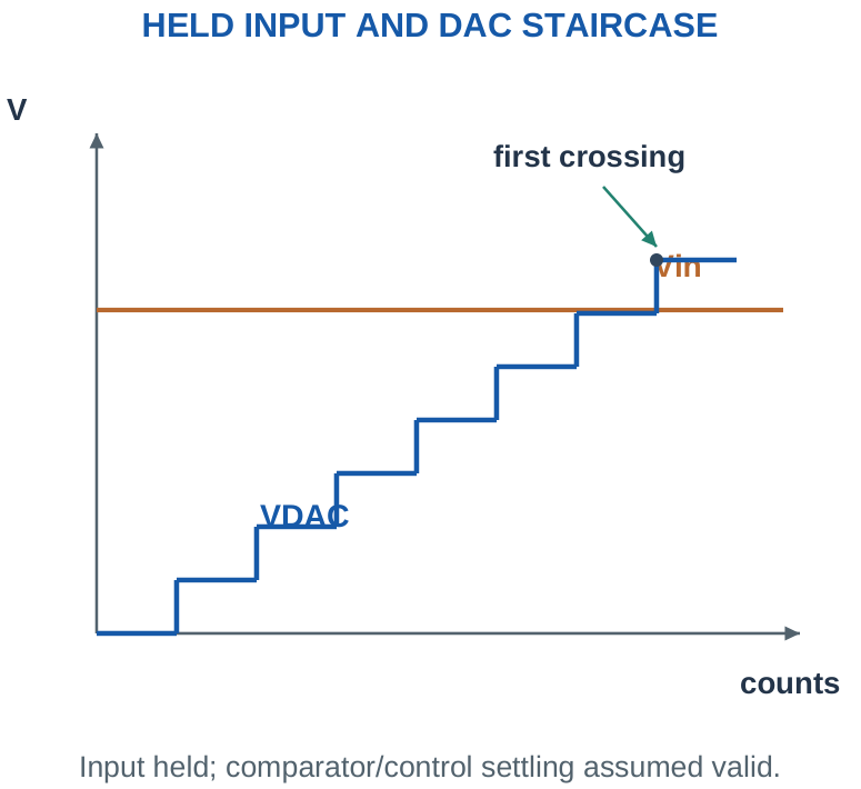
A digital-ramp ADC uses a binary counter, a DAC, a comparator and control logic. Reset the counter, increase its code with a clock, and convert that code into a rising staircase voltage. Compare the DAC voltage with the held or sufficiently slow input. Stop counting when the specified crossing condition is reached and retain the count.
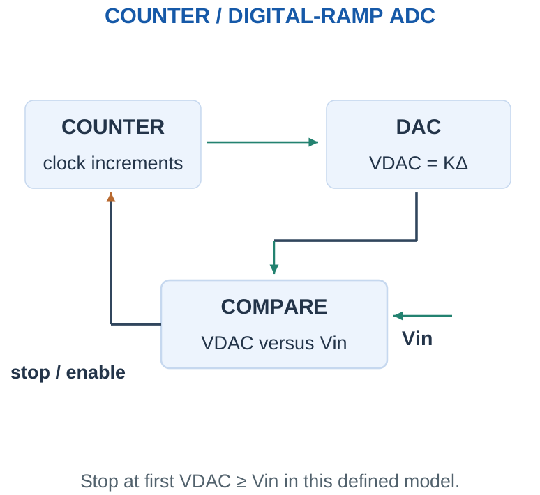
First-crossing convention used here: For these counter examples, VDAC = KΔ, counting starts at zero and stops at the first code satisfying VDAC ≥ Vin. Therefore K = ceil(Vin/Δ) for the stated reachable range. This upper-crossing count differs from the general floor-bin convention used earlier. It is valid because the stop rule is explicitly defined, not because ceil and floor are interchangeable.
At an exactly reachable input KΔ, the count is K. Above the largest reachable DAC voltage, a bounded counter must report over-range rather than wrap. The input must remain stable during the comparison sequence; otherwise the result can be inconsistent.
Architecture cue: One comparator is reused across many trial counts. Conversion time therefore depends on the input level and counter clock.
Worked Problem 5.10: First-Crossing Counter Code
Problem: An N = 8 counter ADC uses Δ = 0.01 V, starts at K = 0 and stops at first KΔ ≥ Vin. Vin = 0.75 V. Find K and final DAC voltage. The input is held constant.
Model / approach: Use the explicitly stated upper-crossing rule K = ceil(Vin/Δ).
Step 1: Vin/Δ = 75; first qualifying integer K = 75.
Step 2: Final VDAC = KΔ = 0.75 V. Previous level = 0.74 V, below the input.
Answer: K = 75; VDAC = 0.75 V.
Check and interpretation: The code fits the stated counter width. For a non-integral Vin/Δ, this first-crossing result can be one code above a floor-bin ADC result; each follows a different explicit threshold convention.
11. Counter Conversion Time and Limitations
If K clock increments are required and clock frequency is fclk, the idealised counting interval is K/fclk. A problem may add reset, settling, latching or other overhead. Worst-case counting needs up to 2^N – 1 increments for the stated N-bit first-crossing model.
Worked check: Worst count is not the bit count
An eight-bit counter ADC can need up to 255 increments under its stated model. At 1 MHz that counting interval is 255 µs, before overhead. It is not eight microseconds merely because the output contains eight bits. A different trial procedure would need its own timing derivation.
The clock cannot simply be made arbitrarily fast: the DAC, comparator and control must settle sufficiently between decisions. The simple K/fclk formula assumes those requirements are already met. It is not a universal timing guarantee for a physical ADC.
An input close to the low end may finish quickly while a high input takes much longer. This makes the architecture straightforward but inefficient when many clock counts are needed. Do not substitute a fixed N-clock binary-search conversion time; that belongs to a different conversion procedure.
Count convention: If counting starts at zero, the count value K corresponds to K increments here. A problem that includes a separate initial comparison or overhead must state how that time is counted.
Worked Problem 5.11: Counting Interval Plus Overhead
Problem: An 8-bit first-crossing counter ADC needs 200 increments at 100000 Hz. Extra reset/latch overhead is 10 µs. Find total conversion time and ideal maximum repeated rate at this input.
Model / approach: Counting takes K/fclk; add overhead before inverting time.
Step 1: Tcount = 200/100000 = 2000 µs.
Step 2: Ttotal = Tcount + overhead = 2010 µs.
Step 3: Ideal repeated rate ≤ 1/Ttotal = 497.5124 conversions/s.
Answer: Ttotal = 2010 µs.
Check and interpretation: The stated clock is assumed slow enough for DAC and comparator settling. Other input levels can need different counts, so this calculated rate is not a constant architecture-wide sample-rate guarantee.
12. Flash ADC: Parallel Comparison
A full flash ADC compares the input with many thresholds simultaneously. An ideal N-bit architecture uses 2^N – 1 comparators. A reference ladder can supply thresholds separated by Δ. An encoder converts the comparator pattern into an N-bit output.
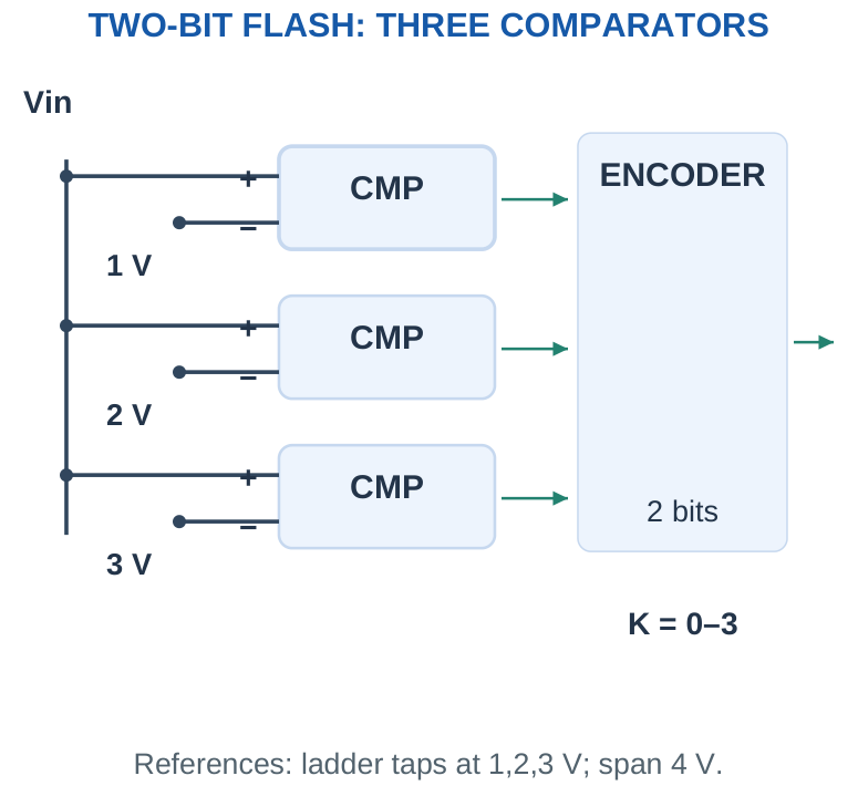
For increasing threshold order, comparator outputs become a run of ones followed by zeros as more thresholds are exceeded. This is a thermometer code. In the educational model, comparator j is HIGH when Vin ≥ jΔ, so the number of crossed thresholds gives the output code, clipped to its maximum. Threshold equality is defined by this model; actual devices have finite transition uncertainty.
Parallel comparison is fast, but comparator count grows exponentially with bit count. Real devices also have input acquisition, comparator delay and encoding delay. A flash ADC does not have zero conversion time and is not automatically the most economical choice for every slow sensor.
Memory cue: N bits gives 2^N codes but 2^N – 1 comparator thresholds in a full flash architecture.
Worked Problem 5.12: Full Flash Hardware Count
Problem: Find the comparator count for a full 3-bit flash ADC. How many output codes are available?
Model / approach: A full flash has one comparator per internal threshold.
Step 1: Comparators = 2^3 – 1 = 7.
Step 2: Output codes = 2^3 = 8.
Answer: 7 comparators; 8 codes.
Check and interpretation: The encoder, ladder, acquisition and control are additional hardware. This count applies to a full flash architecture, not every converter containing a smaller flash stage.
Worked Problem 5.13: Thermometer Code to Binary
Problem: A 3-bit full flash ADC spans 0–4 V with thresholds 0.5, 1.0, 1.5, 2.0, 2.5, 3.0, 3.5 V. Outputs are listed in ascending threshold order and are HIGH when Vin ≥ threshold. Find the pattern and binary code at Vin = 2.6 V.
Model / approach: Count the thresholds crossed, retaining the stated thermometer order.
Step 1: The first five thresholds are crossed and the last two are not. Pattern = 1111100.
Step 2: The crossed-threshold count is 5, so the binary output is 101.
Answer: Thermometer 1111100; code 101.
Check and interpretation: Reversing the list of comparator outputs reverses the printed thermometer pattern without changing the number crossed. State the order before interpreting the bit string.
Worked check: Threshold count versus code count
A two-bit full flash has four output codes and three thresholds. With a 4 V span, nominal thresholds are 1, 2, 3 V in this educational model. At 2.4 V, the ascending-threshold pattern is 110 and its binary code is 10. The number of crossed thresholds is two.
13. Counter-Ramp Versus Flash ADC
| Feature | Digital-Ramp | Full Flash |
|---|---|---|
| Trial process | Successive counter/DAC staircase | Parallel threshold comparisons |
| Comparator use | One reused comparator in basic model | 2^N – 1 comparators |
| Timing | Depends on required count | Parallel comparison plus encoding |
| Main advantage | Straightforward architecture | High conversion speed |
| Main trade-off | Many clocks at high counts | Hardware, area and power grow rapidly |
Do not confuse a digital-ramp counter ADC with a single-slope analog-ramp converter or with successive approximation. All convert analog signals to codes, but their trial generation and timing are different. The syllabus specifically names digital-ramp and flash types; other architectures are useful comparisons but need not replace those two explanations.
Selection depends on required sampling rate, resolution, input behaviour, power and cost. For a slowly varying weather sensor, maximum flash speed may not be useful. For a fast waveform, an input-dependent long counter interval may be unacceptable.
Numerical caution: Comparator count alone does not equal complete circuit component count. Both architectures also need references, control and output handling.
14. Sampling Rate and Data Volume
Sampling records input information at separate times. A sample interval Ts corresponds to sample rate fs = 1/Ts. Conversion time, input acquisition and data transfer can each limit how frequently usable measurements are obtained.
For an ideally band-limited signal with highest frequency fmax, alias-free sampling requires fs greater than 2fmax, with practical margin and an appropriate analog anti-alias filter. This introductory condition does not say that sampling exactly twice an arbitrary waveform frequency guarantees faithful measurement in real hardware.
For several channels, distinguish the per-channel rate from total conversion rate. Four channels at 100 samples/s each need at least 400 conversions/s, before allowing overhead. Stored or transmitted data also includes the allocated bytes per sample and any framing, timestamps or status fields.
Two separate questions: “How small a voltage change?” concerns resolution. “How fast a change over time?” concerns sampling and analog bandwidth.
Worked Problem 5.14: Aggregate Samples and Data Rate
Problem: 4 channels each need 100 samples/s, with 2 stored bytes per sample. Find aggregate conversion rate and raw byte rate without metadata.
Model / approach: Multiply channels by per-channel rate before calculating data volume.
Step 1: Total rate = 4 × 100 = 400 conversions/s.
Step 2: Raw data = 400 × 2 = 800 bytes/s.
Answer: 400 conversions/s; 800 bytes/s.
Check and interpretation: A single shared converter must support the aggregate acquisition/conversion schedule. Headers and timestamps add bytes; a nominal ADC bit count alone does not define stored or transmitted record size.
15. PWM: Period, Duty Ratio and Average
Pulse-width modulation (PWM) controls the fraction of each fixed period spent HIGH. Define duty ratio D = Ton/T, with T = Ton + Toff and frequency f = 1/T. Duty expressed as a percentage is 100D.
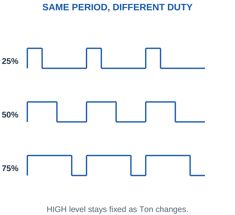
For a waveform switching between VL and VH, its average is Vavg = D VH + (1 – D)VL. For 0-to-VS pulses this becomes DVS. The output is still a pulse waveform; a load’s response or a filter may make its effect look smoother. A GPIO PWM signal is not automatically a precision analog DC source.
For a purely resistive load connected directly to ideal 0-to-VS pulses, average power is D VS²/R and RMS voltage is VS√D. It is wrong to calculate that power from Vavg²/R unless the load actually sees the filtered average voltage rather than the original pulses.
Scope: PWM is treated as a concept and waveform here. No timer register configuration or programming is required.
Worked Problem 5.15: Duty, Frequency and Average Voltage
Problem: Ton = 2 ms, Toff = 8 ms, HIGH = 5 V and LOW = 0 V. Find duty, frequency and average voltage.
Model / approach: Use the full period and both voltage levels.
Step 1: T = 2 + 8 = 10 ms. D = Ton/T = 20%.
Step 2: f = 1/T = 100 Hz.
Step 3: Vavg = D VH + (1 – D)VL = 1 V.
Answer: D = 20%; f = 100 Hz; average 1 V.
Check and interpretation: The output remains a pulse waveform. An average-voltage calculation is not an instruction to replace the original pulsed waveform with a DC source for every power or timing question.
Worked Problem 5.16: RMS and Resistor Power
Problem: Ideal 0-to-10 V pulses with duty 25% drive a 100 Ω resistor directly. Find average voltage, RMS voltage and average power.
Model / approach: Use time-averaged squared voltage for resistor power.
Step 1: Vavg = 0.25 × 10 = 2.5 V.
Step 2: VRMS = 10√0.25 = 5 V.
Step 3: Pavg = D VS²/R = 0.25 × 100/100 = 0.25 W.
Answer: Vavg = 2.5 V; VRMS = 5 V; Pavg = 0.25 W.
Check and interpretation: Using Vavg²/R gives 0.0625 W, which would apply to a resistor seeing a steady 2.5 V instead. The stated load sees the original full-height pulses.
16. PWM in Motor and LED Control
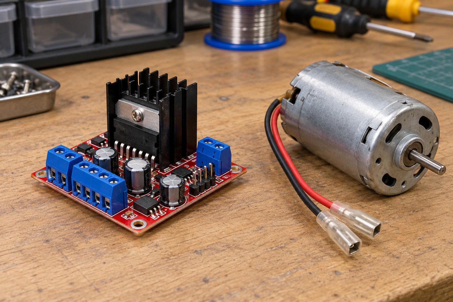
A low-power PWM output can command a transistor or driver that switches a larger load supply. The signal controls timing; the driver handles load voltage and current. Motor winding inductance and mechanical inertia influence the response, so duty ratio is not a universal exact speed formula.
Worked check: PWM frequency is not duty
At a period of 1 ms, frequency is 1000 Hz. Ton = 0.2 ms gives 20% duty, while Ton = 0.8 ms gives 80%. Both use the same frequency. Changing pulse width within a fixed period changes average drive without necessarily changing the waveform repetition rate.
Worked check: Average current needs a waveform model
If a supplied ideal load draws 100 mA only during ON and zero during OFF, 30% duty gives average current 30 mA. A motor winding may continue carrying current during OFF through its recirculation path. The same simple zero-OFF-current calculation cannot be assumed for that motor without a model.
TIMING BOUNDARY
PWM: Include ON plus OFF time in the period.
UART: Include framing intervals.
SPI: Count the required shifted sequence once.
I2C: Count the supplied address/data and acknowledgement clocks.
A wire-time estimate excludes unspecified scheduling, gaps, retries and processing.
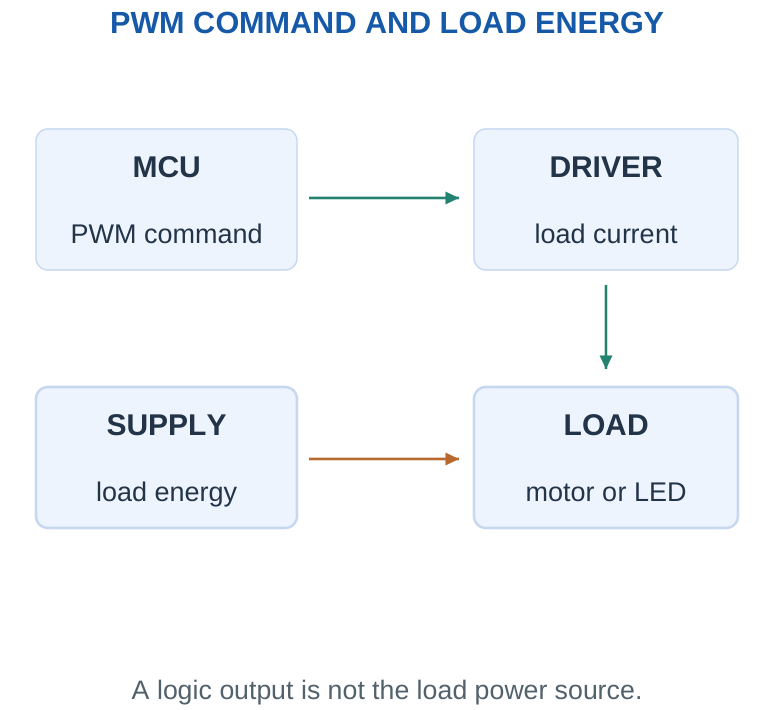
For an LED, short pulses and visual integration can control apparent brightness, but LED current still needs a defined limit. Brightness may not be exactly proportional to duty over every device and observation condition.
For a motor, current, back EMF, load torque and recirculation paths matter. A supplied ideal average-voltage model can estimate DVS. Label it as a model rather than a guaranteed measured motor speed. A switch’s conductive loss can be estimated with given ON resistance and current, but varying current and switching losses need their own data.
Driver check: An acceptable PWM duty does not establish voltage compatibility or load-current capability. Verify command levels and load path separately.
17. UART: Asynchronous Serial Communication
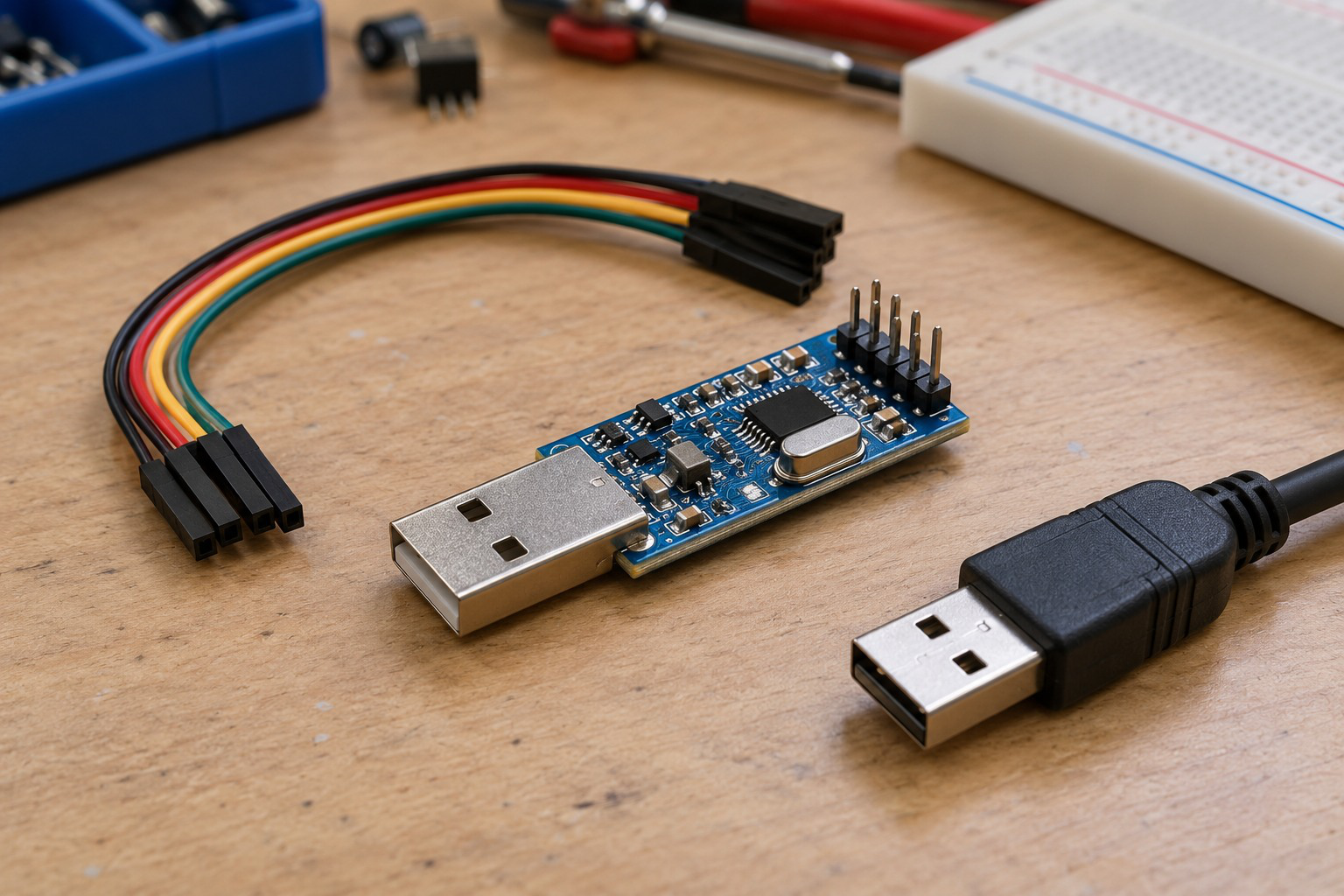
A UART exchanges serial data without a shared clock wire. The transmitting and receiving ends agree on bit rate and frame format. A common format is 8N1: one start bit, eight data bits, no parity and one stop bit, giving ten transmitted bits per byte.
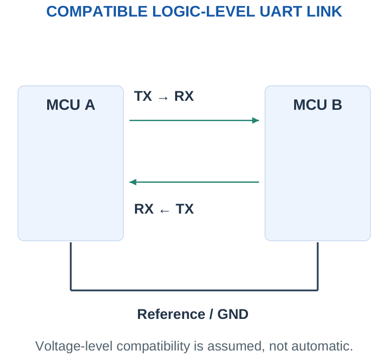
An idle logic-level UART line is normally HIGH. A LOW start bit announces a frame, followed by data and a HIGH stop interval in this model. Separate TX and RX paths can support simultaneous transfer. A basic UART frame does not itself provide a network address or guarantee error-free delivery.
In binary UART signalling, one symbol carries one bit, so the stated baud rate equals the bit rate in the examples here. Adding parity or extra stop bits increases frame length and reduces the payload fraction at the same bit rate.
Interface distinction: UART describes the serial peripheral and framing. USB, RS-232 and RS-485 require additional appropriate interface hardware and are not identical to a bare MCU TX/RX connection.
Worked Problem 5.17: Count UART Framing Overhead
Problem: A UART frame has one start bit, 8 data bits, 0 parity bit and 1 stop bit. Find total bits and data-bit fraction.
Model / approach: Count every transmitted interval.
Step 1: Frame length = 1 + 8 + 0 + 1 = 10 bits.
Step 2: Data fraction = 8/10 = 80%.
Answer: 10 transmitted bits; 80% are data bits.
Check and interpretation: This fraction excludes application-level headers, inter-frame gaps and retries. A frame’s data fraction and a complete message’s useful sensor payload fraction can therefore differ.
18. UART Throughput and Packet Timing
If every frame contains F transmitted bits and baud rate is B, one frame takes F/B seconds. A packet of M such bytes needs MF/B seconds when sent back-to-back with no gaps. The payload byte rate for 8N1 is B/10, not B/8.
Worked check: One byte takes more than eight UART bits
At 9600 baud with 8N1, one byte occupies ten bit intervals, taking 10/9600 ≈ 1.0417 ms. Eight data bits alone occupy 0.8333 ms, but that excludes required framing. A no-gap stream therefore carries at most 960 payload bytes/s under this format.
Worked check: Check headroom in a data link
A 1000-byte/s payload requires 10,000 bit/s with 8N1 before headers. A supplied 19,200-baud link passes that basic capacity check; 9600 baud does not. The faster link still needs allowance for gaps and any extra packet fields. A theoretical pass is not a complete timing measurement.
If a sample produces several bytes, multiply sample rate by bytes per sample and then by transmitted frame bits per byte. Add application headers, checksums or separators when specified. A link with exactly the required theoretical rate has no allowance for scheduling gaps or retries.
A UART can be adequate for a debugging port, a nearby module or low-rate telemetry. It is not a direct substitute for a radio link or an addressed multi-device bus. System-level communication needs a compatible electrical layer and an agreed interpretation of the byte stream.
Common error: A rate written in bits/s cannot be compared directly with a requirement written in bytes/s. Convert units and include framing before judging capacity.
Worked Problem 5.18: UART Packet Transfer Interval
Problem: Send 20 bytes back-to-back at 9600 baud with 10 transmitted bits per byte. Find ideal packet time and payload byte rate.
Model / approach: Assume binary signalling, no gaps and no extra packet fields.
Step 1: Transmitted bits = 20 × 10 = 200.
Step 2: Time = bits/baud = 20.8333 ms.
Step 3: Payload byte rate = baud/10 = 960 bytes/s.
Answer: Packet interval ≈ 20.8333 ms.
Check and interpretation: The calculation includes the supplied frame overhead. It is a lower bound on elapsed application time if scheduling gaps, retransmissions or additional fields occur.
19. SPI: Clocked Peripheral Communication
Serial Peripheral Interface (SPI) uses a controller-provided clock and data paths between controller and peripheral. Common names are SCK for clock, MOSI for controller-to-peripheral data, MISO for peripheral-to-controller data and CS for device selection. COPI/CIPO are alternative direction names.
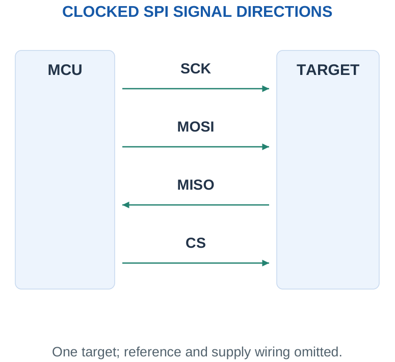
A conventional four-wire SPI link can transfer one bit in each direction per clock, so shifting one byte takes eight clock cycles without extra gaps. Simultaneous incoming and outgoing bits do not automatically make useful payload throughput twice the requested one-way data rate; command bytes and device behaviour matter.
Several peripherals may share clock and data lines with separate selects when their outputs release appropriately while unselected. SPI has no universal address, frame size or acknowledgement scheme built into every device’s transfer convention. Its clock polarity and sampling phase must be compatible.
Scope: Know what SPI does and what its wires mean. These notes use stated bit counts and clock rates rather than detailed register or timing-mode programming.
Worked Problem 5.19: SPI Shift Timing
Problem: A transaction shifts 3 total bytes at SCK = 1000000 Hz. Every byte takes 8 clocks. No gaps or extra command bytes are needed beyond this stated total. Find shift time.
Model / approach: Count all specified bytes once in the serial clock sequence.
Step 1: Clocks = 3 × 8 = 24.
Step 2: Tshift = 24/1000000 = 24 µs.
Answer: Shift interval = 24 µs.
Check and interpretation: Full duplex can shift a bit in each direction on the same clock, but the required command/response sequence determines useful data. Do not double the number of clocks merely because both directions are active.
20. I2C: Shared Addressed Two-Wire Bus
I2C connects devices through a serial data line SDA and serial clock line SCL. In common standard/fast-mode arrangements, lines are open drain and use pull-ups, allowing devices to pull LOW or release the line. A controller addresses the intended target on the shared bus.
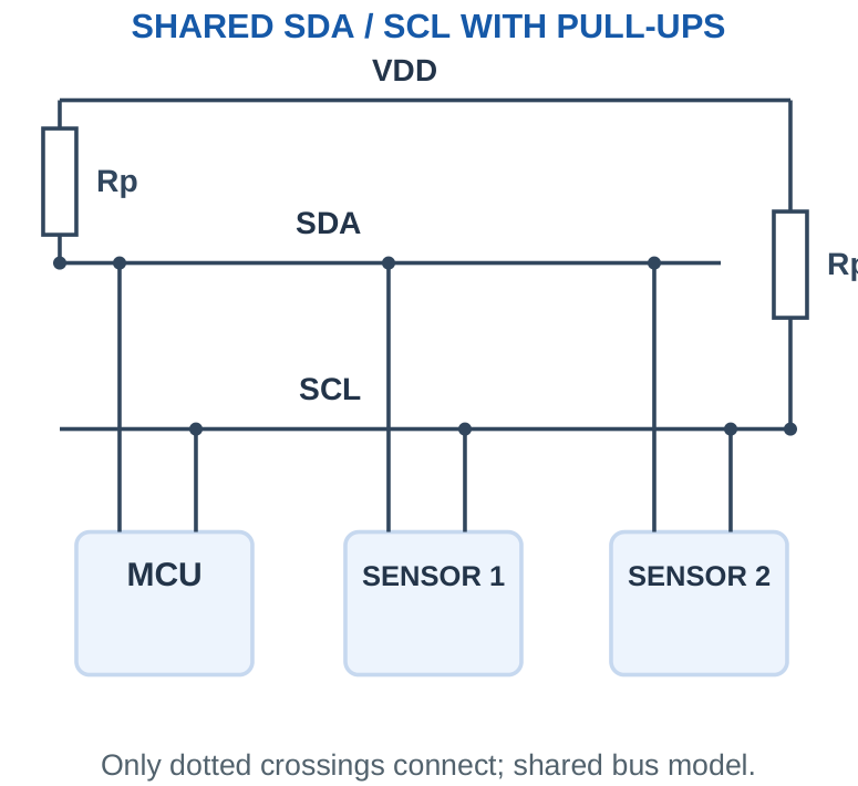
Data transfers include address/control and acknowledgement information, so bus clock frequency is not equal to useful bytes per second. A simplified calculation may count eight data bits plus one acknowledgement clock per byte, with address bytes and other overhead included as stated.
A seven-bit address label is different from an eight-bit address-plus-direction value appearing in a transaction. Do not assign two indistinguishable targets the same fixed address on the same unsegmented bus. Pull-up value depends on allowed sink current and line capacitance; it is not a universal constant.
Practical cue: Two signal wires does not mean no ground or supply reference is needed. The devices still require compatible electrical levels and references.
Worked Problem 5.20: Simplified I2C Transfer Budget
Problem: A supplied I2C transaction model has 4 transmitted bytes total, including its stated address/control bytes. Count 8 bits plus 1 ACK clock per byte at SCL = 100000 Hz. Ignore START/STOP timing, stretching and gaps. Find clocked interval.
Model / approach: Use the explicitly supplied nine-clock-per-byte model.
Step 1: Clocks = 4 × 9 = 36.
Step 2: Tclocked = 36/100000 = 360 µs.
Answer: Clocked interval = 360 µs.
Check and interpretation: This is not a complete protocol timing guarantee. If a read’s final byte uses NACK instead of ACK, its ninth clock is still counted in this simple interval model.
21. Choosing UART, SPI or I2C
| Interface | Timing/Control | Typical Role |
|---|---|---|
| UART | Asynchronous frames; TX/RX | Point-to-point module or console link |
| SPI | Shared clock, separate selection | Sensor, ADC, display or memory transfer |
| I2C | Shared addressed SDA/SCL bus | Several nearby sensors or control ICs |
Worked check: SPI full duplex shares clocks
A stated full-duplex SPI exchange shifts eight clocks while one byte goes out and one byte comes in. Its shift interval at 1 MHz is 8 µs, not 16 µs. Whether both bytes contain useful payload depends on the device transaction; command and response scheduling must still be specified.
Worked check: Sensor offset must be removed
A sensor gives vS = 0.5 + 0.01T volts. At T = 25 °C it gives 0.75 V. Multiplying that voltage by 100 without subtracting the 0.5 V intercept would report 75 °C. The correct inverse is T = (vS – 0.5)/0.01.
UART is simple for a compatible pair of endpoints. SPI can provide efficient clocked transfer but often uses more selection pins as the number of targets grows. I2C saves signal wires for addressed devices but needs compatible addresses and bus loading. These are broad architectural comparisons, not universal speed limits for every implementation.
Ask whether the sensor already outputs a digital measurement. A digital sensor with an internal converter may send a code directly over I2C or SPI, so it does not require an extra external op-amp and ADC in the same path. An analog sensor typically needs the analog chain before the controller can process a numerical sample.
Answer with reasons: A good selection answer states the required data rate, target count, available pins and device support. Naming an interface without those connections is incomplete.
22. Sensor-to-Controller Signal Chain
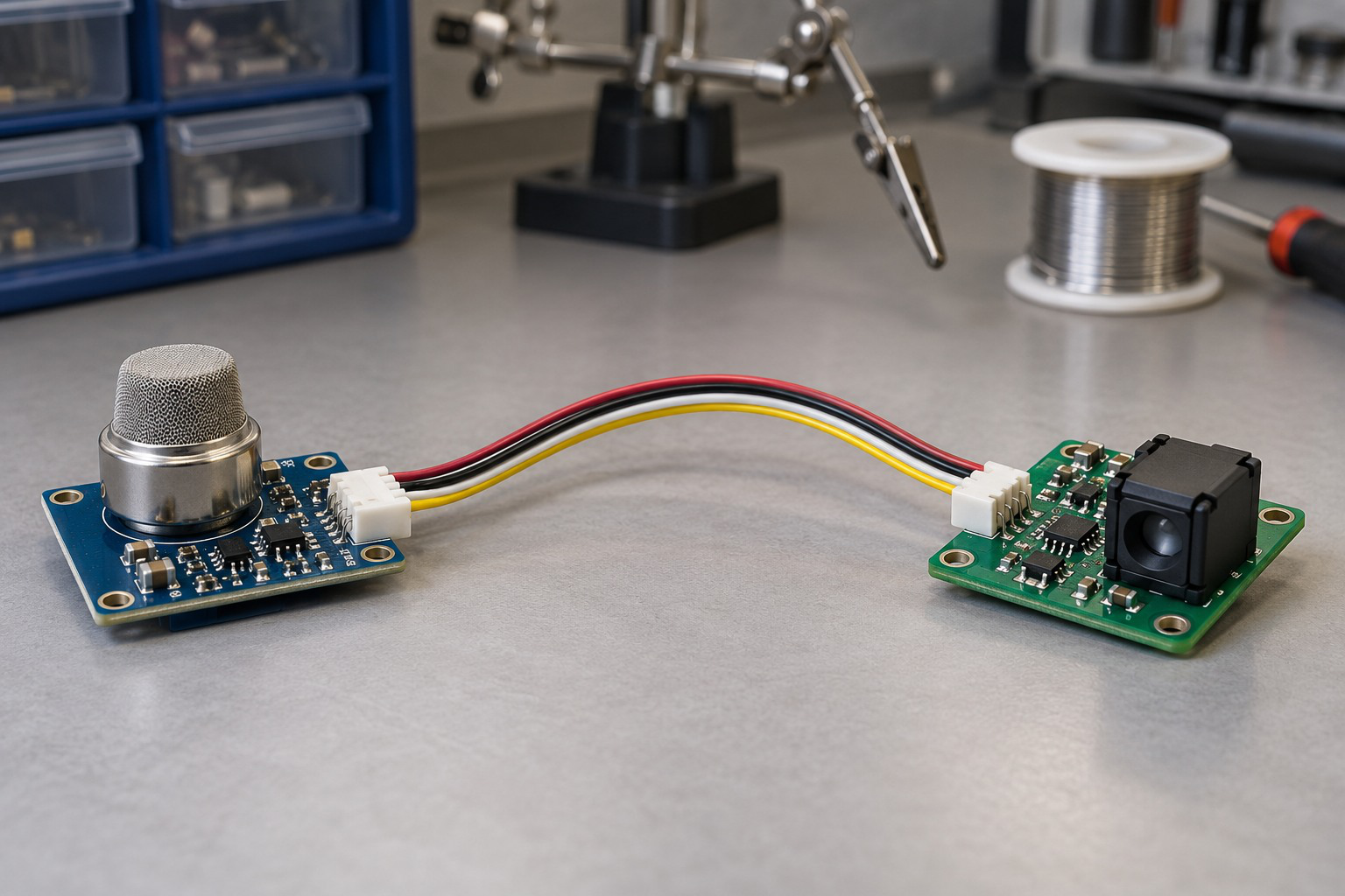
The generic analog chain is sensor → conditioning → ADC → microcontroller. A sensor produces an electrical response. Conditioning can provide amplification, offset adjustment, filtering and buffering. The ADC maps voltage into a code, and the controller applies calibration and decision logic.
Worked check: Endpoint consistency
A desired mapping from 0.5–1.5 V to 0.5–3.0 V has slope 2.5 and intercept -0.75 V. Substitution gives 0.5 V at the lower input and 3.0 V at the upper input. Matching only the upper endpoint does not prove that a simple gain-only circuit is correct.
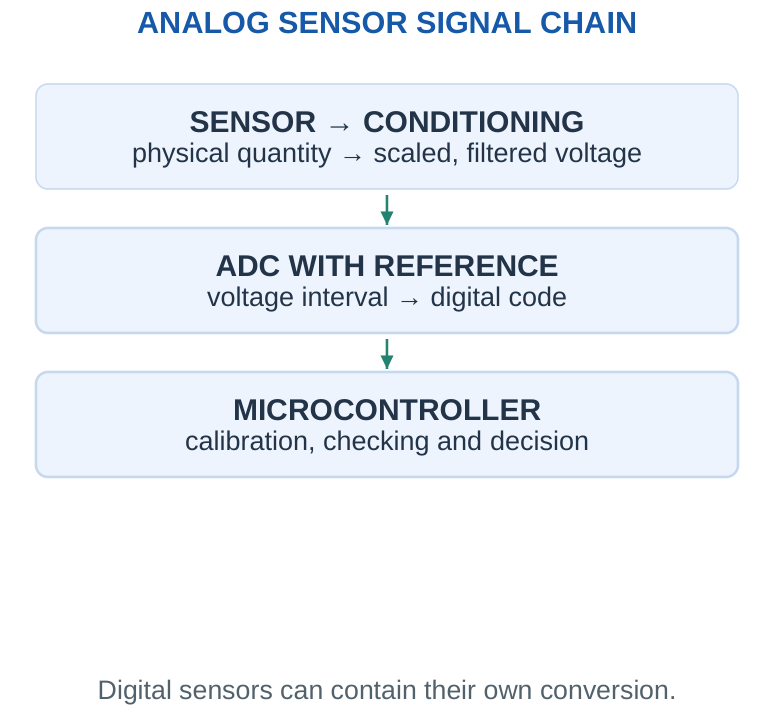
The sensor may have an offset and non-unit sensitivity. A conditioning stage must match both slope and intercept to the required ADC range. Check source loading, common-mode input range and output headroom; an ideal gain formula alone does not prove the chain is usable.
For a stated model vS = Sx + b and conditioning vo = GvS + c, the overall relation is vo = GSx + Gb + c. The inverse physical estimate uses the same calibration coefficients. Applying raw ADC voltage directly as a physical quantity without those coefficients gives wrong units.
Range habit: Calculate the voltage at every stage at both physical endpoints. A later stage cannot recover information that an earlier stage clipped.
Worked Problem 5.21: Design a Gain-and-Offset Transfer
Problem: Map sensor voltage 0.2–0.8 V to 0.5–3.0 V at an ADC. Find vo = GvS + c and midpoint output. Assume a suitable conditioning circuit and valid ranges.
Model / approach: Use both endpoints to determine slope and intercept.
Step 1: G = (3.0 – 0.5)/(0.8 – 0.2) = 4.1667.
Step 2: c = 0.5 – G × 0.2 = -0.3333 V.
Step 3: At sensor midpoint 0.5 V, vo = 1.75 V.
Answer: vo = 4.1667vS + (-0.3333 V).
Check and interpretation: An ordinary ground-referenced gain stage cannot independently supply every offset c. The algebra defines the required transfer; choose a topology that implements it and check its common-mode and output ranges.
23. Calibration and Physical Interpretation
Two known calibration points determine an ideal linear relationship. If a measured electrical value y corresponds to physical x, slope a = (y2 – y1)/(x2 – x1) and intercept b = y1 – ax1. Then x = (y – b)/a when a is nonzero.
For a temperature sensor with 10 mV/°C sensitivity and a 0.5 V zero-temperature offset, 0.9 V represents 40 °C in the stated model. Multiplying 0.9 V by a guessed constant without removing the offset gives an incorrect result. Calibration units must remain explicit.
A nominal numerical mapping is different from a validated instrument accuracy claim. Sensor tolerance, reference variation, conditioning error, quantisation and installation conditions can contribute. If only one of these is supplied, report that contribution rather than inventing a complete guaranteed error.
Revision trick: Check the computed physical value by substituting it back into the forward sensor equation. This quickly detects sign, scale and intercept mistakes.
Worked Problem 5.22: Recover Temperature from an Offset Sensor
Problem: The stated sensor model is vS = 0.5 V + (10 mV/°C)T. Measured vS is 0.9 V. Find T.
Model / approach: Subtract the intercept before dividing by sensitivity.
Step 1: Useful voltage = 0.9 – 0.5 = 0.4 V.
Step 2: T = (vS – b)/S = 40 °C.
Answer: T = 40 °C in the stated linear calibration.
Check and interpretation: Substitution into vS = ST + b recovers the given voltage. This result assumes the model applies over the temperature interval; it is not a complete real sensor accuracy claim.
24. Bluetooth and Bluetooth Low Energy
Bluetooth supports wireless communication between compatible nearby devices. Bluetooth Low Energy (LE) is particularly useful for short data exchanges and low-duty-cycle connected sensors, including wearables. It should not be treated as identical to every other Bluetooth operating mode.
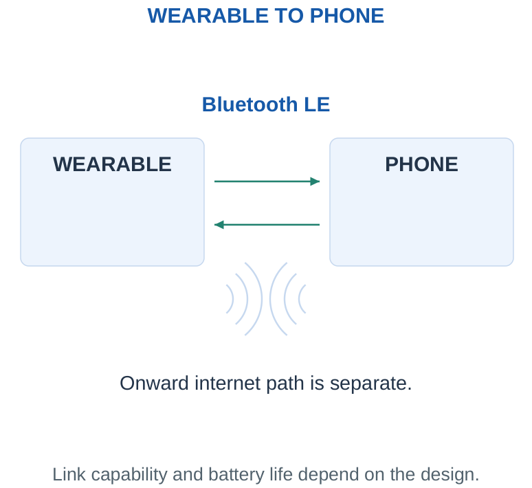
A low-power radio label does not determine complete battery life. Advertising, connection timing, transmit intervals, receive listening, retries and application duty cycle all affect energy. A sensor that sleeps most of the time may use far less average current than one that continuously transmits, even with the same radio hardware.
Bluetooth is not automatically an internet connection. A phone or gateway can forward data onward if the application provides that route. Range depends on radio settings, antennas, obstruction and environment, so a universal fixed distance is not assumed in these notes.
Choice clue: For a wearable sending modest measurements to a phone, Bluetooth LE is a plausible conceptual choice when both ends support the required service and power budget.
25. Wi-Fi in Connected Electronic Systems
Wi-Fi commonly connects a device to a local network through an access point, allowing communication with other local devices or internet services when the network provides access. It can support relatively data-rich applications, but energy use depends strongly on activity and implementation.
Worked check: Separate sampling from reporting
A node may sample once per second but transmit a batch once per minute. With four bytes per record, a complete minute stores 240 raw bytes. The reporting rate is one batch per minute, while the local sampling rate remains one sample per second. Batching trades latency and memory for fewer sessions.
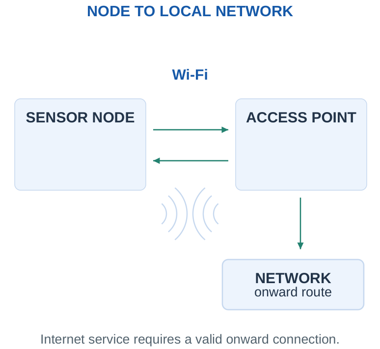
For a weather station, Wi-Fi can send readings to a network dashboard without requiring a nearby phone to remain the gateway. However, association, listening and transmission intervals can affect a battery-powered node’s average energy. Duty cycling, buffering several readings and choosing update intervals are useful system-level trade-offs.
Do not compare technologies using one universal speed, range or current number. The numerical problems supply an assumed current and active time specifically for a calculation. Packet overhead, signal conditions and retries can reduce payload efficiency and increase energy.
System question: Does the application need direct local-network access, a nearby phone link or a multi-node low-rate mesh? The intended communication path helps choose a suitable technology.
26. Zigbee and Low-Power Mesh Networks
Zigbee is used for low-rate sensing and control networks, often with mesh communication through suitable powered routing devices. It is useful in smart-home and building applications where many small nodes exchange status and control information.
Worked check: A router has a different role
A battery end sensor can sleep between reports when its network behaviour permits it. A router expected to forward other devices’ traffic normally needs availability for that role. Applying the same sleepy-node current budget to every router can underestimate total network demand even when payload rates are low.
Worked check: Forwarded payload adds
If three nodes each report 16 payload bytes every 8 s through a router, the raw forwarded rate is 3 × 16/8 = 6 bytes/s. This excludes link overhead, receive listening and retransmissions. A low useful byte rate does not prove that the router consumes negligible power.
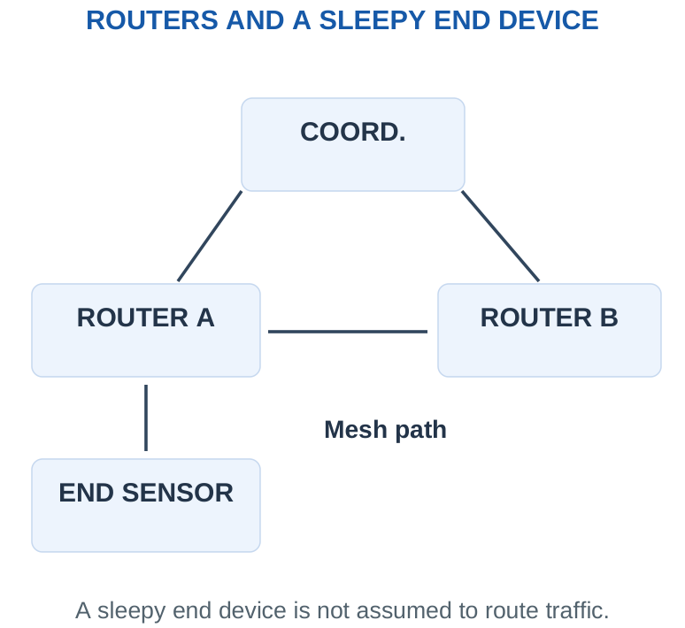
A coordinator establishes or manages network functions in the conceptual model. Routers extend communication paths. End devices can focus on their own sensing and may sleep according to their supported operation. Sleeping is a system behaviour, not a guarantee that every role has the same low average power.
Mesh can provide alternative paths when supported by placement and routing, but it does not make a network immune to interference or poor coverage. More hops may add delay and consume energy at routing nodes. A gateway is needed when the Zigbee network must exchange data with another network or internet service.
Compare fairly: A phone may support Bluetooth and Wi-Fi directly but usually needs a compatible gateway or coordinator path for a Zigbee installation. Check endpoints rather than assuming all wireless radios communicate with each other.
27. Wireless Selection and Reporting Duty Cycle
| Need | Plausible Conceptual Option |
|---|---|
| Wearable to nearby phone | Bluetooth LE |
| Sensor to local-network dashboard | Wi-Fi |
| Many low-rate home sensor nodes | Zigbee with suitable network roles |
Worked check: Do not add overlapping currents twice
If a supplied 30 mA active-state figure already includes the MCU and radio together, adding another 10 mA MCU current to it would double-count part of the state. Average complete operating states, or sum genuinely separate simultaneous blocks, according to the stated measurement boundary.
The weighted-average current model is Iavg = Σ(Ii ti)/T over a complete operating cycle. Include every defined state: sensing, processing, transmitting, receiving and sleeping. If currents already include overlapping blocks, do not add those same block currents again.
Ideal runtime from a battery capacity C in mAh and average battery-side current in mA is C/Iavg hours. Real runtime can differ because of usable capacity, converter losses, self-discharge, temperature and cutoff. When currents refer to another voltage rail, compare energy or convert through efficiency instead of mixing currents from different voltages directly.
Numerical condition: All radio currents and transfer times used here are supplied illustrative assumptions, not measured performance promises for a named technology or product.
Worked Problem 5.23: Duty-Cycled Average Current and Runtime
Problem: Battery-side current is 20 mA for 0.1 s of every 10 s, and 0.02 mA for the rest. Battery capacity is 1000 mAh. Find average current and ideal runtime.
Model / approach: All currents are already at the battery boundary; no extra converter penalty is added.
Step 1: Iavg = [20 × 0.1 + 0.02 × 9.9]/10 = 0.2198 mA.
Step 2: Runtime = 1000/Iavg ≈ 4549.5905 h = 189.5663 days.
Answer: Iavg ≈ 0.2198 mA; ideal runtime ≈ 4549.5905 h.
Check and interpretation: The capacity is assumed fully usable at the stated conditions. Real cutoff, self-discharge, temperature and uncounted events can shorten runtime. Do not report this ideal model as guaranteed field life.
28. LDO Regulation and Dropout
A low-dropout regulator (LDO) is a linear regulator that controls its pass element to maintain an output voltage while operating with a relatively small required input-output difference. “Low dropout” describes a minimum headroom condition under specified load and temperature, not zero voltage difference.
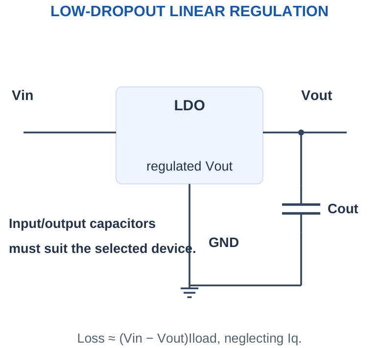
To maintain a requested output, require Vin ≥ Vout + Vdropout under the stated conditions. If input falls below that requirement, the output is no longer guaranteed to remain at its nominal value. Exact dropout behaviour depends on the device and load.
Ignoring quiescent current, efficiency is approximately Vout/Vin and dissipation is (Vin – Vout)Iload. Including quiescent current Iq gives input power Vin(Iload + Iq). An LDO does not normally boost a lower input into a higher regulated output.
Selection balance: LDO simplicity and low output noise can be useful, but a large voltage drop at significant current creates heat and poor efficiency.
Worked Problem 5.24: Dropout Headroom Test
Problem: Vin = 3.7 V, desired Vout = 3.3 V and supplied dropout requirement = 0.2 V at the load. Does the headroom condition pass?
Model / approach: Require Vin ≥ Vout + Vdropout.
Step 1: Minimum needed input = 3.3 + 0.2 = 3.5 V.
Step 2: Headroom margin = 3.7 – 3.5 = 0.2 V.
Answer: Headroom condition passes.
Check and interpretation: Dropout depends on the specified load and conditions. Passing this voltage test does not establish allowable thermal dissipation or output-current capability.
29. LDO Power and Thermal Estimates
A first power check uses Pout = Vout Iload and Ploss ≈ (Vin – Vout)Iload, or includes Iq when provided. Thermal rise can be estimated as ΔT ≈ Ploss θJA using a supplied junction-to-ambient resistance. Junction temperature is then approximately ambient temperature plus that rise.
A quoted θJA depends on package, PCB copper, airflow and test arrangement. It is not a universal property independent of installation. Compare the calculated temperature with a supplied permitted value, retaining appropriate margin in a real design. Thermal shutdown is a last protection feature, not a normal operating target.
For a sensor rail, small current and a modest drop may make an LDO reasonable. For a large load powered from a much higher voltage, a switching converter may reduce loss. Noise and power can sometimes be balanced with a switching pre-regulator followed by an LDO, but the LDO still needs headroom.
Do both checks: Enough dropout headroom does not prove an LDO stays cool. A low thermal rise does not prove its input voltage is sufficient for regulation.
Worked Problem 5.25: Loss, Efficiency and Thermal Estimate
Problem: Vin = 12 V, Vout = 3.3 V, Iload = 0.1 A, θJA = 60 °C/W and ambient = 25 °C. Ignore Iq; supplied allowable junction limit is 125 °C. Estimate loss, efficiency and junction temperature.
Model / approach: Use the stated steady thermal model and assume dropout/current conditions otherwise pass.
Step 1: Ploss = (12 – 3.3) × 0.1 = 0.87 W. η ≈ Vout/Vin = 27.5%.
Step 2: Rise ≈ Ploss θJA = 52.2 °C.
Step 3: Tj ≈ 25 + 52.2 = 77.2 °C; below the supplied 125 °C limit.
Answer: Loss 0.87 W; estimated Tj 77.2 °C.
Check and interpretation: The given θJA applies only under its assumed mounting conditions. A result below the limit is a preliminary calculation rather than proof of practical thermal margin in every board layout.
30. DC-DC Converters: Buck and Boost Concepts
A switching DC-DC converter uses controlled switching and energy-storage components to change DC voltage. A buck converter steps voltage down. A boost converter steps it up. Some topologies can provide an output above or below the input. These functions differ from an LDO’s dissipative voltage reduction.
Worked check: Converter currents need not match
An ideal 12 V to 3 V converter supplying 1 A has output power 3 W and input current 3/12 = 0.25 A. At supplied 80% efficiency, input power becomes 3.75 W and input current 0.3125 A. The reduced voltage permits larger output current while respecting energy balance.
Worked check: Buck duty is an ideal ratio
For the supplied steady ideal buck model, 12 V to 3.3 V requires D = 3.3/12 = 0.275 or 27.5%. That ratio alone does not specify switch current, inductor ripple or a controller. A real design must remain within the selected converter’s duty and operating limits.
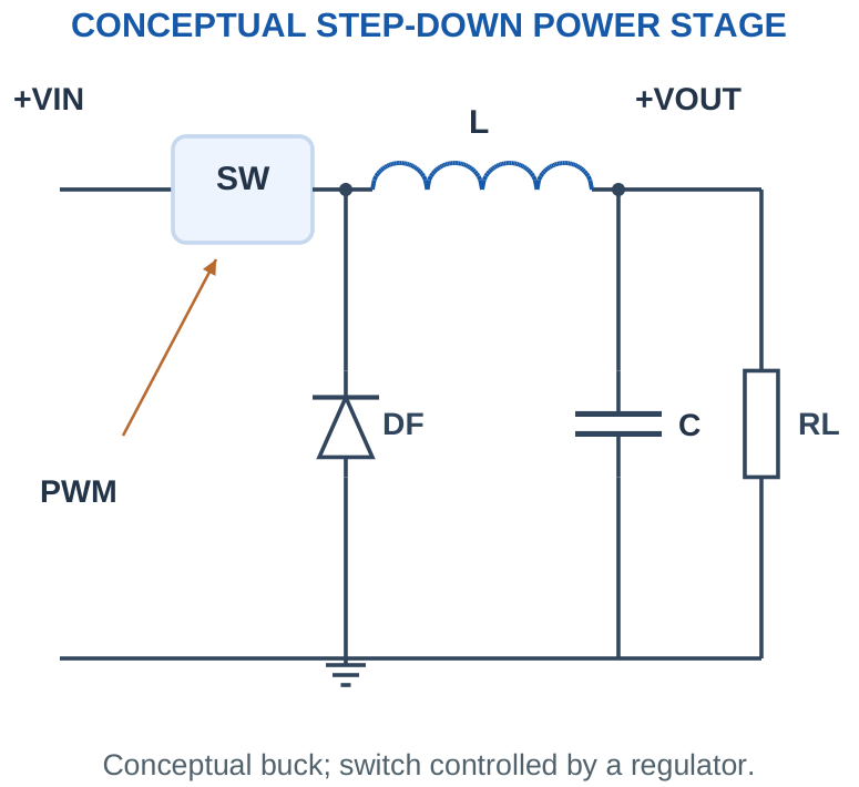
For an ideal buck in steady continuous-conduction operation, Vout = DVin. For the corresponding ideal boost model, Vout = Vin/(1 – D). These are introductory model equations, not universal formulas for every load, topology, switching limit or discontinuous operating state.
With given efficiency η, Pin = Pout/η and input current is Pin/Vin. Output current can be larger than input current in a step-down converter because voltage changes while energy is conserved apart from loss. Equal input and output current is not a general switching-converter rule.
Physical distinction: A switching regulator can be efficient without being lossless. Ripple, switching noise, current limits and control behaviour remain important in a practical power system.
Worked Problem 5.26: Converter Power and Input Current
Problem: A stated converter supplies 3.3 V at 0.2 A from 12 V with efficiency 90%. Find output/input power, input current and loss.
Model / approach: Use power conversion rather than equating input and output currents.
Step 1: Pout = 3.3 × 0.2 = 0.66 W. Pin = Pout/η = 0.7333 W.
Step 2: Iin = Pin/Vin = 0.0611 A. Ploss = Pin – Pout = 0.0733 W.
Answer: Iin ≈ 61.1111 mA; loss ≈ 0.0733 W.
Check and interpretation: The supplied efficiency is assumed valid at this operating point. Voltage conversion changes the input/output current relationship, while energy balance accounts for the loss.
Worked Problem 5.27: Ideal Buck Duty Ratio
Problem: For a stated ideal buck model, convert 12 V to 5 V. Find duty. Assume steady continuous conduction and ignore losses.
Model / approach: Use Vout = D Vin for buck or Vout = Vin/(1 – D) for boost.
Step 1: D = 5/12 = 0.4167.
Step 2: Duty percentage = 41.6667%.
Answer: Ideal duty ≈ 41.6667%.
Check and interpretation: This ideal ratio does not select a physical controller, inductor, switch or current rating. Maximum duty, startup and discontinuous operation can alter a practical converter’s behaviour.
31. Power Budget, Energy and Ideal Runtime
Power is energy per time. Electrical power at a DC rail is VI. Battery energy in watt-hours is approximately nominal voltage times ampere-hours under a stated simplified model. Capacity in mAh is a charge quantity, so it cannot be compared directly across different operating voltages as if it were energy.
Worked check: Ah and Wh are different
A nominal 3.7 V, 2 Ah battery has approximately 7.4 Wh in the simplified nominal model. The same 2 Ah rating at 7.4 V corresponds to 14.8 Wh. Equal charge capacity does not imply equal energy when the nominal voltage differs.
Worked check: Usable fraction and efficiency
For nominal energy 10 Wh, usable fraction 80% leaves 8 Wh at the battery boundary. A supplied 90% conversion efficiency delivers 7.2 Wh to the load. A constant 0.3 W load then has an estimated 24 h runtime. Include each boundary loss once and state the ideal assumptions.
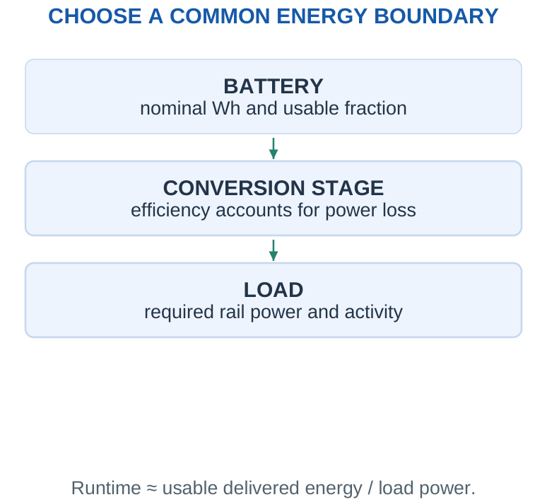
For a regulated constant-power load, usable battery energy divided by load power, with conversion efficiency included consistently, gives an idealised runtime. For same-voltage battery-side current states, use weighted average current and C/Iavg. Do not apply both a battery-side measured current and a second converter penalty to the same loss already included.
A peak-current requirement is separate from an average-energy requirement. A battery system can have enough nominal energy yet fail to support radio or motor current pulses. Startup and sleep currents may differ strongly from the normal active current.
Report honestly: State ideal or estimated runtime and its assumptions. A calculated number of hours is not a guarantee of field battery life.
Worked Problem 5.28: Runtime from a Regulated Power Load
Problem: Battery nominal voltage = 3.7 V, capacity = 2 Ah, usable fraction = 80%, converter efficiency = 90% and constant load power = 0.2 W. Estimate runtime.
Model / approach: Use usable watt-hours and include conversion loss once.
Step 1: Usable battery energy ≈ 3.7 × 2 × 0.8 = 5.92 Wh.
Step 2: Energy delivered to load ≈ ηE = 5.328 Wh.
Step 3: Runtime ≈ ηE/Pout = 26.64 h.
Answer: Estimated runtime ≈ 26.64 h.
Check and interpretation: Nominal voltage times capacity is a simplified energy model. Actual discharge voltage, cutoff and temperature can change usable energy; this is not a guaranteed battery specification.
32. IoT Weather-Station Architecture
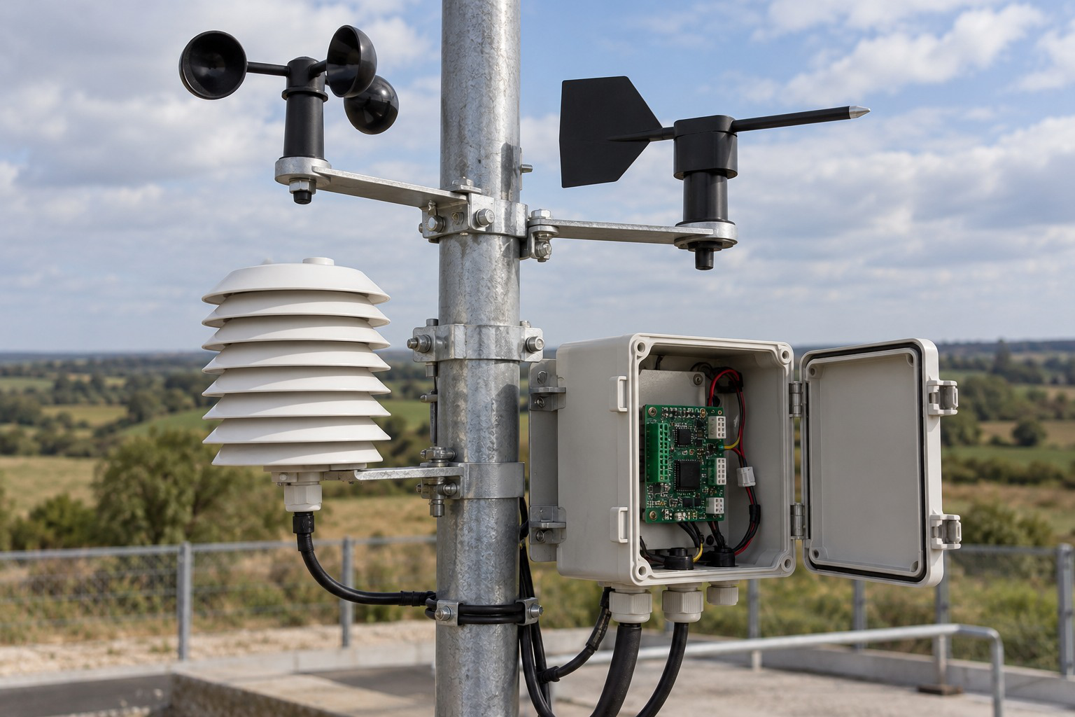
A weather station can measure temperature, humidity and pressure, then record or transmit readings. Analog sensors use conditioning and conversion as needed. Digital sensors may report already converted measurements over a supported serial interface.
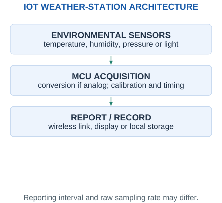
An MCU schedules readings, applies calibration, checks plausible ranges and packages data. Wi-Fi can connect to a local network, while other radio choices may use a gateway. Time stamps and status flags help distinguish a new valid reading from a stale or failed measurement.
A sampling interval for slow weather changes need not match a high-rate radio capability. Buffering several readings before transmission can reduce the number of radio wakeups, at the cost of delayed reporting and memory use. Outdoor measurement quality also depends on sensor placement and environmental protection; electronics alone does not establish meteorological accuracy.
Explain the path: Identify which sensors are analog and which are digital. Do not place an unnecessary second ADC after a digital sensor’s I2C output.
Worked Problem 5.29: Weather-Station Data Buffer
Problem: 4 sensor channels are recorded 2 times/s, each using 2 bytes per reading. Store 5 minutes without metadata. Find total readings and raw storage.
Model / approach: A record contains one reading from each channel.
Step 1: Records = 2 × 60 × 5 = 600. Total individual readings = 2400.
Step 2: Storage = records × channels × bytes = 4800 bytes.
Answer: 4800 raw bytes.
Check and interpretation: Timestamps, validity flags, indexing and communication buffers would need extra storage. A digital sensor’s packet may also contain more than the two bytes retained as the measurement.
33. Smart-Home Sensor Node
A smart-home node may read a door switch, light level, temperature or occupancy signal and send an event or periodic report. A suitable low-power network can connect multiple nodes through a controller or gateway. An actuator node may additionally operate a lamp, lock or relay through an appropriate driver.
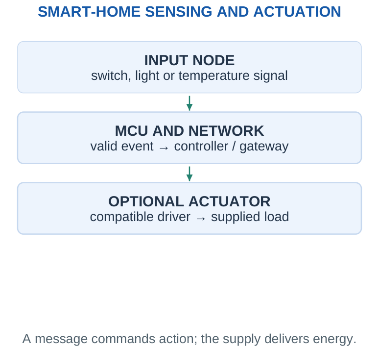
For a battery door sensor, an active-LOW switch input and sleep-between-events behaviour are useful concepts. For a light-controlled lamp, an analog signal chain or comparator can make a threshold decision. Hysteresis can prevent repeated switching near the threshold.
Network roles and supply matter: a constantly available router normally has a different energy budget from a sleepy end sensor. Reporting every input edge may be unsuitable for a bouncing switch; the system should interpret valid events rather than raw contact chatter.
System-level check: A received radio message does not itself provide actuator power. The controller’s decision, logic interface, driver and load supply must all be accounted for.
34. Wearable Health-Device Electronics
A wearable can combine a physiological or motion sensor, a suitable analog front end, an ADC, an MCU and a wireless link to a phone. Battery size, skin-contact conditions and movement make power management and signal quality particularly important.
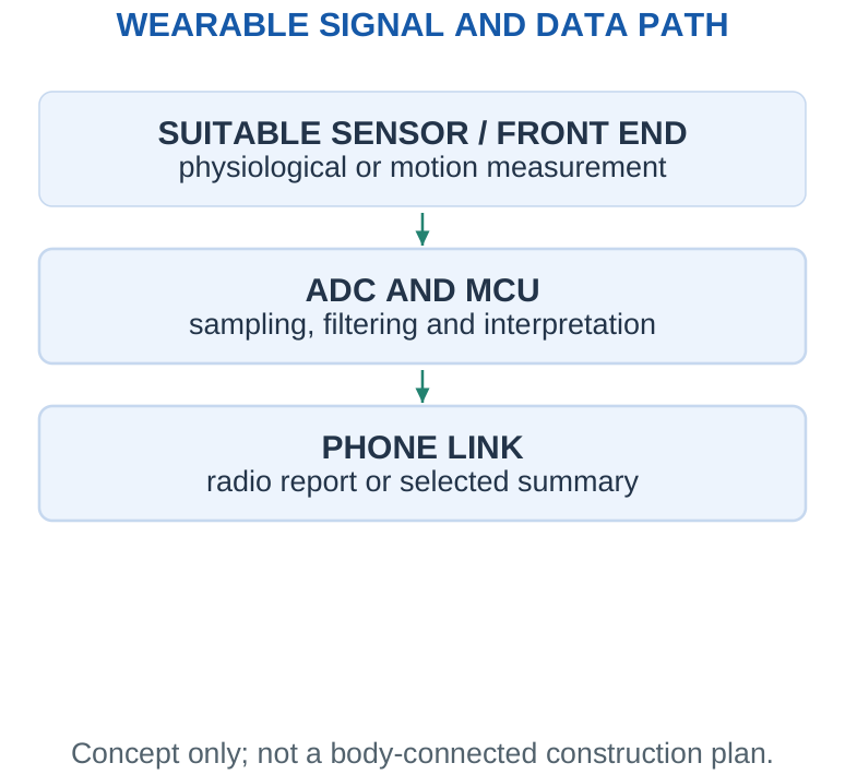
An ECG-type signal uses a specialised biopotential front end with differential sensing and appropriate protection. An optical pulse sensor uses light emitters and photodetection. These are different measurement methods and should not be described as interchangeable raw circuits.
Filtering and processing can reduce unwanted components and extract useful information, but motion artefacts, poor contact and ambient effects can still degrade results. A classroom signal-chain calculation does not establish diagnostic accuracy. Actual body-connected electronics require specialised protection and isolation considerations appropriate to their design.
Bluetooth LE is a plausible phone-link choice. Duty-cycled acquisition and reporting can save energy, but the measurement must still retain the required time resolution. Sending fewer summaries is not equivalent to preserving every original raw sample.
Keep the claim limited: Use the supplied abstract voltage, sampling and power models for numerical learning. Do not infer a clinical diagnosis from an educational code or waveform calculation.
35. EV Battery-Management-System Overview
An EV battery-management system (BMS) supervises a battery pack using cell-voltage, current and temperature measurements. It supports protection decisions, estimation of state of charge, cell balancing and communication with other vehicle systems. The pack’s charger, inverter and BMS are related but distinct functions.
TRACE THE COMPLETE NODE
Measurement: Sensor, readout, scale and validity.
Processing: Correct decision and state.
Communication: Supported route and timing.
Power: Every rail and load path.
Action: Feedback showing the response achieved.
A network connection does not establish measurement accuracy or actuator operation.
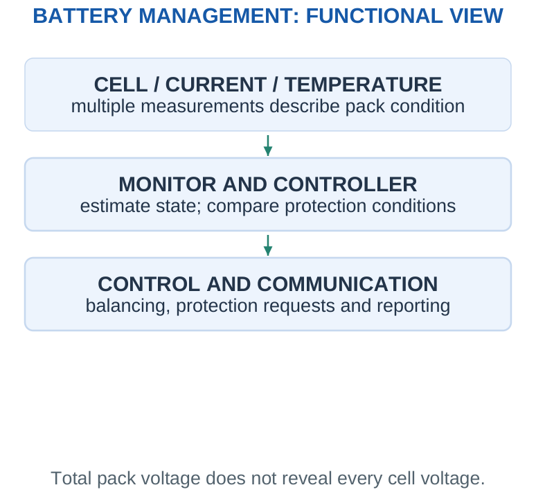
Series cells add voltage; parallel cells add charge capacity under an ideal matched-cell model. Total pack voltage alone cannot reveal whether one series cell is over-voltage or under-voltage, so individual cell or cell-group monitoring matters. State of charge (SOC) is an estimate of remaining charge relative to a defined capacity, not simply “pack voltage percentage”.
Passive balancing removes energy from selected higher-charge cells through dissipative paths. Active balancing transfers energy using additional circuitry. Neither creates extra battery energy. Coulomb counting integrates current over time but needs a valid initial estimate and correction for errors and operating conditions.
Scope: This is a functional overview with low-level mathematical examples. It is not a wiring or commissioning procedure for a high-voltage EV battery pack.
Worked Problem 5.30: Ideal Series-Parallel Pack Arithmetic
Problem: A hypothetical matched-cell model uses 4 cells in series per string and 2 strings in parallel. Each cell is nominal 3.7 V, 2.5 Ah. Find cell count, pack nominal voltage, capacity and energy.
Model / approach: Series adds voltage; matched parallel strings add capacity.
Step 1: Cells = 4 × 2 = 8. Voltage = 4 × 3.7 = 14.8 V.
Step 2: Capacity = 2 × 2.5 = 5 Ah. Nominal energy = V × Ah = 74 Wh.
Answer: 14.8 V, 5 Ah; nominal 74 Wh.
Check and interpretation: This is arithmetic under a matched ideal model, not an assembly instruction. Real pack configuration, protection, current sharing and monitoring require a defined battery-system design.
36. [B] PLC: Industrial Input, Logic and Output
A programmable logic controller (PLC) acquires field inputs, executes stored control logic and commands industrial outputs. Its processor, memory, input/output modules, power supply and communication interfaces form a controller system rather than a single bare microcontroller chip.
Inputs may be discrete states from switches/proximity sensors or analog measurements through suitable modules. Outputs may be relay, transistor or other specified interfaces. A logical ON command must be matched to the load voltage, current and switching requirements; the output image is not the motor energy supply.
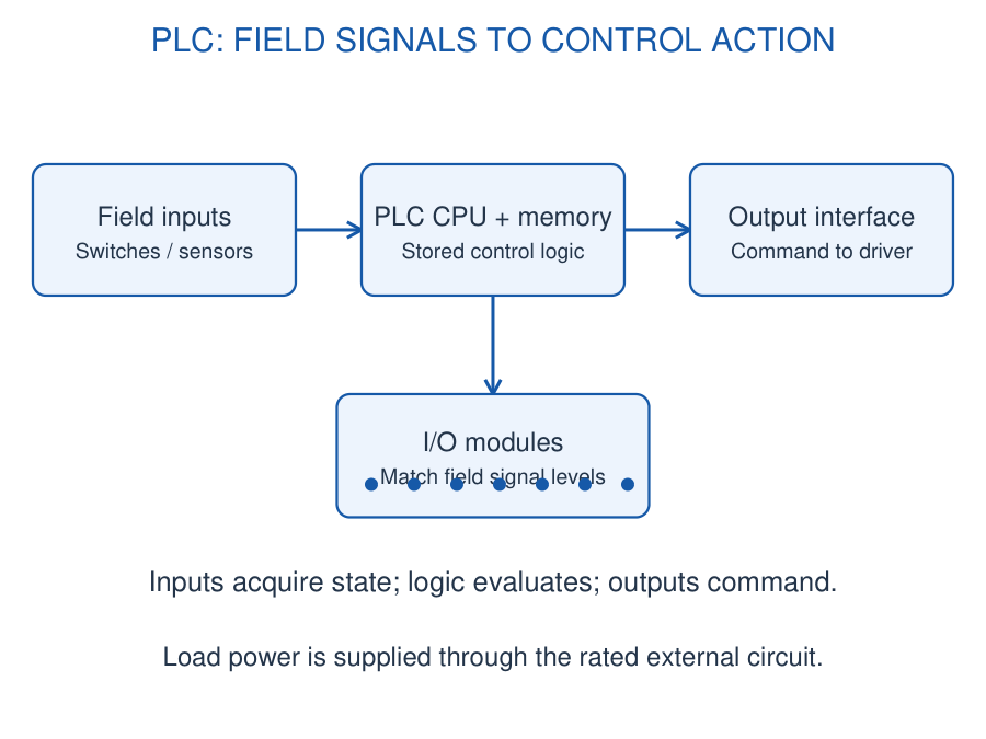
Ladder concept: Series conditions represent AND, parallel branches represent OR, and a complemented contact instruction tests a false Boolean. Define whether each variable means request, permission or active fault before writing the rung. A normal-open instruction is true for a stored 1; this does not by itself specify the physical switch wiring.
A cyclic execution model reads relevant inputs, evaluates the logic and updates outputs along with diagnostics and communication. Exact update order and direct-I/O behaviour are controller dependent. Input snapshots explain why a physical transition may not appear immediately in the logic being executed.
Application: A motor permit M = R AND NOT F allows a run request only when the declared fault is absent. State memory, interlocks and timers add functions beyond this combinational expression. A teaching rung is not a complete safety-rated emergency-stop circuit.
Worked Problem 5.31: PLC Motor Permit
Problem: R = 1 means run request and F = 1 means active fault. Use M = R AND NOT F. Evaluate (R,F) = (1,0), (1,1), (0,0).
Model / approach: Apply the declared input meanings.
Step 1: The first pair gives 1 AND 1 = 1.
Step 2: The second has NOT F = 0; the third has R = 0.
Answer: M = 1, 0, 0.
Check: This logical rule does not alone specify a safety-rated stop circuit.
Worked Problem 5.32: PLC Input Capacity
Problem: A controller has 16 discrete input channels. Nine switches and five proximity outputs each use one channel. Find used and spare channels.
Model / approach: Count independently assigned compatible inputs.
Step 1: Used = 9 + 5 = 14.
Step 2: Spare = 16 – 14 = 2.
Answer: 14 used; 2 spare discrete inputs.
Check: Analog channels, special functions and output capacity require separate checks.
37. [B] VFD: Rectifier, DC Bus and Inverter
A variable frequency drive (VFD) supplies a suitable AC motor with a controlled electrical frequency and voltage. Its introductory power path is AC input → rectifier → DC bus → inverter → motor. The controller and gate drivers command the power switches.
The rectifier converts the incoming AC into DC. The DC bus/link includes energy storage and filtering that support the inverter. The inverter uses controlled semiconductor switching to synthesise an AC output with the required fundamental frequency and voltage.
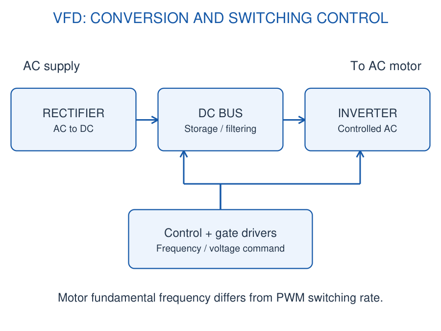
For a rotating field with P poles, synchronous speed is ns = 120f/P revolutions per minute. An induction motor normally runs below synchronous speed while motoring because it requires slip. A frequency command therefore does not universally equal measured rotor speed.
PWM switching frequency and motor fundamental frequency are different quantities. A drive may switch many times during one motor-current cycle. Control adjusts frequency/voltage or more detailed motor variables according to its design; a block diagram does not establish a universal control law.
Reading the diagram: Distinguish the high-power conversion path from the low-power command and feedback paths. Motor current/temperature and drive conditions can feed protection and control. A conventional diode-front-end drive does not automatically return braking energy to the mains.
Worked Problem 5.33: VFD Frequency and Rotating-Field Speed
Problem: A four-pole rotating field is supplied at 50 Hz and then 40 Hz. Find both synchronous speeds.
Model / approach: ns = 120f/P.
Step 1: At 50 Hz: ns = 120 × 50/4 = 1500 rpm.
Step 2: At 40 Hz: ns = 120 × 40/4 = 1200 rpm.
Answer: 1500 rpm and 1200 rpm synchronous speed.
Check: An induction motor rotor speed also depends on slip; the computed values are not guaranteed shaft speeds.
Worked Problem 5.34: Stored DC-Link Energy
Problem: For an abstract capacitor model, C = 1000 µF and V = 100 V. Find stored energy.
Model / approach: E = CV²/2; convert µF to F.
Step 1: C = 0.001 F.
Step 2: E = 0.5 × 0.001 × 100².
Answer: 5.0 J.
Check: This is an energy calculation, not an operational procedure for a drive.
38. [B] SCADA and HMI: Supervisory Information
SCADA means supervisory control and data acquisition. It collects information from controllers or remote terminal units, presents process status, records trends/alarms and can issue authorised supervisory commands. Field control normally occurs through suitable local controller logic.
A human-machine interface (HMI) is the operator-facing screen or panel for values, alarms, status and commands. SCADA is a broader supervisory system; an HMI can be a local panel without being an entire SCADA installation.
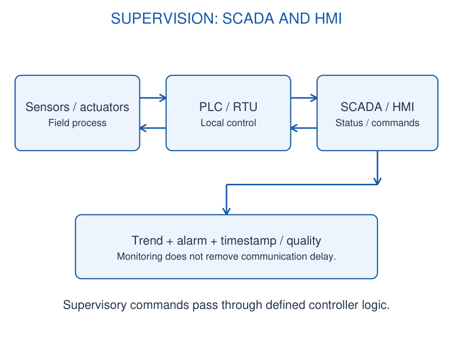
Information path: Sensor → field I/O → PLC/RTU → communication network → supervisory system/HMI. Commands travel back through an authorised interface to the controller, which applies relevant permissions and local logic before updating outputs.
Display freshness depends on acquisition, communication, polling and processing delays. A recently refreshed screen can still contain an invalid measurement. Include timestamps, units, quality flags and clear loss-of-communication indications.
Remote monitoring allows values to be observed away from equipment; it does not guarantee instant response or a continuous connection. Alarms, access permissions and command confirmation must follow the actual system requirements. A dashboard is not a replacement for the complete field control and protection architecture.
Worked Problem 5.35: HMI Refresh Rate
Problem: A panel refreshes a displayed channel every 0.5 s. Find refresh frequency and the maximum extra wait caused only by this periodic refresh.
Model / approach: f = 1/T; consider a change immediately after a refresh.
Step 1: f = 1/0.5 = 2 Hz.
Step 2: A change just after one refresh waits almost 0.5 s for the next.
Answer: 2 Hz; refresh-related wait from 0 up to almost 0.5 s.
Check: Acquisition, network and processing delays are additional.
39. [B] Wireless Sensor Networks and Industrial IoT
A wireless sensor network contains sensing nodes that acquire local measurements and communicate them to another node or gateway. A node combines sensor/readout, processing, communication and power. Network topology may be star, mesh or another supported arrangement.
Industrial IoT (IIoT) links industrial measurements and equipment information with networked analysis or supervision. A gateway can translate local interfaces, aggregate readings and forward selected data to plant or remote services. Connecting a sensor to a radio does not alone complete this system.
Choose reporting interval, latency, reliability and power budget together. Battery nodes often sleep between measurements; a forwarding router may need to stay available and therefore have a different energy requirement. Buffering supports temporary loss of connectivity but requires defined storage and timestamps.
Industrial constraints: Metallic structures, interference, electrical noise, temperature and mounting affect performance. Select a supported communication technology for the required range, traffic and environment. Authentication, access control and maintenance are part of a deployed system, not properties guaranteed by the word wireless.
Example: A temperature node and a motor-vibration node send time-stamped values to a gateway. The gateway forwards a trend or alarm while retaining the identity and validity of each channel. Sensor calibration and network connectivity answer different questions.
Worked Problem 5.36: IIoT Report Traffic
Problem: Twenty nodes each send one 24-byte payload every 10 s. Find mean payload bytes/s at a gateway, ignoring overhead and retries.
Model / approach: Aggregate the same declared traffic boundary.
Step 1: Each node contributes 24/10 = 2.4 bytes/s.
Step 2: Total = 20 × 2.4.
Answer: 48 payload bytes/s.
Check: Protocol overhead, bursts and retransmissions increase required link capacity.
40. [B] Smart Manufacturing and Motor Condition Monitoring
Condition monitoring observes indicators of equipment condition over time. A motor node may measure vibration, temperature or current and compare features against a baseline. A changing indicator can prompt inspection; it is not automatically a unique diagnosis.
A vibration sensor, often an accelerometer, converts motion into an electrical signal. Mounting orientation, attachment stiffness, sensor range, bandwidth and calibration influence the result. A loose sensor can change the recorded vibration without a change in the motor itself.
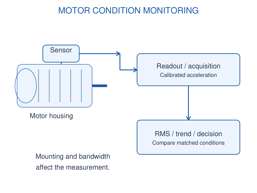
Chain: Sensor → conditioning/anti-alias filter → acquisition → feature calculation → trend/decision → maintenance indication. Useful features can include RMS amplitude and frequency content. Compare like operating speeds and loads when interpreting trends.
For samples representing a zero-mean calibrated acceleration, RMS = square root of the mean of squared sample values. A DC bias should be distinguished from the vibration component when the objective is AC vibration RMS. The worked example states its sample convention.
Smart manufacturing uses such measurements with controller and production information to support monitoring and maintenance. A threshold is meaningful only with a declared baseline, measurement bandwidth, units and decision objective. Preserve raw/derived data as appropriate for later investigation.
Worked Problem 5.37: Vibration Sample RMS
Problem: A calibrated zero-mean acceleration sequence is +2, -2, +2, -2 m/s². Find RMS.
Model / approach: Square, average and take the square root.
Step 1: Squared values are 4,4,4,4. Mean square = 4 (m/s²)².
Step 2: RMS = √4.
Answer: 2.0 m/s² RMS.
Check: The signed arithmetic mean is zero, but the vibration amplitude is not.
41. [C] ECG Machine: Electrodes to Displayed Waveform
An ECG records electrical potential differences associated with cardiac activity. Electrodes couple the small signal to a differential analog front end; amplification and filtering prepare it for conversion and recording.
Block chain: Electrodes → protected differential amplifier → suitable filtering → ADC → processing → display/storage. The display shows a waveform against time, while acquisition and calibration establish the amplitude and timing scales.
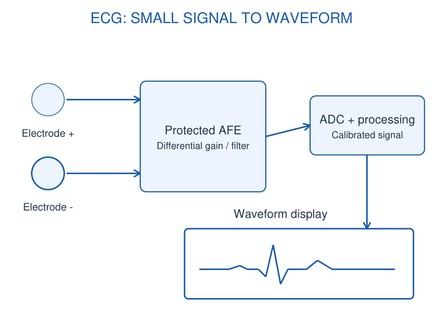
High input impedance reduces loading. Common-mode rejection helps suppress interference common to both inputs, but electrode imbalance, motion and offsets can still corrupt the signal. Allocate gain so that unwanted offsets do not saturate the first stage before filtering.
Sampling rate and converter resolution must suit the required signal bandwidth and amplitude range. Digital processing can reduce selected artefacts or extract features, but cannot recover information already clipped or aliased at acquisition.
Concept boundary: The block diagram explains information flow, not a patient-connected construction design. Protection, leakage control and isolation belong to the complete appropriate medical system. A plotted waveform alone does not prove signal quality or support a diagnosis.
Worked Problem 5.38: ECG Signal Scaling
Problem: A supplied 2 mV differential test signal must give 1 V. Find ideal total gain, ignoring offset for this calculation.
Model / approach: Gain = output/input.
Step 1: 2 mV = 0.002 V.
Step 2: G = 1/0.002.
Answer: 500 V/V.
Check: A real front end must additionally check offset, noise, input range and output headroom.
Worked Problem 5.39: ECG Acquisition Storage
Problem: Two channels are sampled at 500 samples/s each for 10 s. Each sample uses 2 bytes. Find samples and raw data bytes.
Model / approach: Count channels, rate, duration and storage width.
Step 1: Samples = 2 × 500 × 10 = 10000.
Step 2: Bytes = 10000 × 2.
Answer: 10000 samples; 20000 raw bytes.
Check: Metadata, headers and transmission framing are excluded.
42. [C] Pulse Oximeter: Optical Sensing and Processing
A pulse oximeter estimates oxygen saturation using optical measurements and a validated processing/calibration method. Red and infrared emitters illuminate tissue, and a photodetector converts received light into an electrical signal.
The analog front end drives the emitters and measures the small detector signal; timing can separate red, infrared and ambient-light contributions. Pulsatile components carry information associated with the pulse. Processing estimates SpO2 and pulse rate and evaluates signal quality.
Block chain: LED drive → tissue interaction → photodiode/readout → ADC → calibrated processing → quality/status → display. A photodiode alone does not directly output an oxygen percentage, and the ratio of two arbitrary raw light readings is not a universal saturation formula.
The display can show saturation in percent and pulse rate in beats per minute. Motion, weak optical signals, ambient interference and other conditions can affect the estimate. Invalid or stale readings need an appropriate status indication rather than being silently treated as current data.
Worked Problem 5.40: Pulse Period to Rate
Problem: A processed pulse waveform has a supplied period 0.8 s. Find pulse rate in beats/min.
Model / approach: Rate = 60/period for this regular teaching waveform.
Step 1: Rate = 60/0.8.
Answer: 75 beats/min.
Check: This arithmetic does not validate the optical signal or interpret a clinical condition.
43. [C] Glucometer: Biosensor, Conversion and Display
A glucometer measures a sample using a validated sensor chemistry and instrument calibration. In an electrochemical example, a reagent-based test strip acts as the biosensor and produces a measurement current under controlled electrical conditions.
The analog front end applies the required electrode potential and measures the response. A transimpedance amplifier converts current to voltage; an ADC digitises it. The processor applies calibration and compensation before displaying the result with its declared unit.
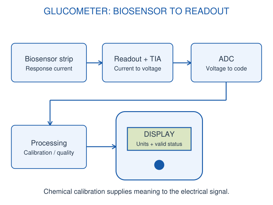
Block chain: Biosensor/test strip → controlled electrochemical readout → current-to-voltage stage → ADC → calibration/quality checks → display. Sample sufficiency, strip condition, temperature and timing can affect the measurement.
For an explicitly supplied linear teaching calibration I = I0 + kG, the concentration estimate is G = (I – I0)/k. This relation is an assumed calibration for the numerical example, not a universal strip equation. A voltage gain alone does not establish the chemical concentration.
Unit discipline: Report the unit defined by the measurement and calibration. Do not change a unit label without converting the value. The following exercises concern instrument signal scaling and do not interpret a clinical result.
Worked Problem 5.41: Supplied Glucose-Sensor Calibration
Problem: A teaching calibration is I = 100 nA + (2 nA per mg/dL)G. Current is 400 nA. Find G.
Model / approach: Subtract the calibration offset before dividing by sensitivity.
Step 1: Net current = 400 – 100 = 300 nA.
Step 2: G = 300/2.
Answer: 150 mg/dL under this supplied calibration.
Check: The relationship is an explicit example, not a universal test-strip model or clinical interpretation.
Worked Problem 5.42: Current-to-Voltage Magnitude
Problem: A transimpedance stage has Rf = 20 MΩ and input current magnitude 50 nA. Find ideal output-change magnitude.
Model / approach: |ΔVout| = |I|Rf.
Step 1: 20 MΩ = 20 × 10^6 Ω.
Step 2: |ΔVout| = 50 × 10^-9 × 20 × 10^6.
Answer: 1.0 V magnitude.
Check: The sign depends on current direction and the chosen reference; check available output swing.
44. [C] Portable Ultrasound: Pulse, Echo and Image
Ultrasound uses high-frequency sound and received echoes to examine internal structures. A piezoelectric transducer converts an electrical excitation into sound and converts returning pressure variations into an electrical signal.
Block chain: Timing/control → transmit pulser → transducer → tissue/target → echo reception → low-noise amplification/filtering → ADC → processing → image/display. A transmit/receive switching arrangement separates the excitation and sensitive receive functions as required by the design.
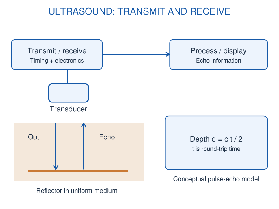
If sound speed is approximated as c and an echo returns after round-trip time t, the reflector depth is d = ct/2. Division by two accounts for travel to the reflector and back. Tissue-dependent sound speed and propagation effects limit this simple model.
A multi-element system can use timed transmit/receive channels and beamforming to form directional information. Processing combines echo timing/amplitude into an image. Portable systems integrate this acquisition and computation with compact power and display arrangements.
Frequency, attenuation, bandwidth and aperture affect image formation; a depth calculation alone does not describe image quality or resolution. The numerical examples use the supplied uniform-speed approximation and do not imply a complete medical instrument design.
Worked Problem 5.43: Ultrasound Echo Depth
Problem: Use sound speed c = 1540 m/s and round-trip echo time 40 µs. Find reflector depth in the stated uniform-medium model.
Model / approach: d = ct/2.
Step 1: t = 40 × 10^-6 s.
Step 2: d = 1540 × 40 × 10^-6/2 = 0.0308 m.
Answer: 30.8 mm.
Check: The factor of two accounts for outward and return propagation.
Worked Problem 5.44: Difference in Echo Depth
Problem: Two echoes differ in round-trip arrival time by 5 µs. Use c = 1540 m/s. Find the depth difference.
Model / approach: Δd = c Δt/2 under the stated model.
Step 1: Δd = 1540 × 5 × 10^-6/2 = 0.00385 m.
Answer: 3.85 mm depth difference.
Check: This does not by itself specify the instrument’s axial resolution.
45. [C] Solar Charge Controller: Energy and Regulation
A solar charge controller manages power transfer from a photovoltaic source to a battery according to the battery requirements and available solar input. It is distinct from a battery monitor, although the two functions can exchange information.
Block chain: PV panel → suitable switching/conversion stage → battery; voltage/current/temperature sensing → controller → switching command. Regulated auxiliary supplies support sensing, processing and communication. Any load connection follows the actual controller architecture.
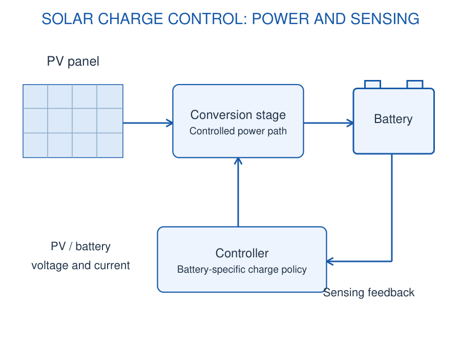
A PWM controller connects/control-switches the charging path according to its design. An MPPT system adjusts the PV operating point to seek available maximum power and uses a conversion stage to match the battery side. Their input/output operating behaviour is not identical.
Charging limits and stages depend on battery chemistry, manufacturer requirements and operating conditions. Include the required overcharge, overdischarge, reverse-current and temperature-related functions in a complete design. Solar input power is variable and not guaranteed by the panel nameplate at every moment.
Energy reasoning: Use a consistent power boundary and stated conversion efficiency. Output power is not the same as output voltage, and panel current need not equal battery current through a switching converter. A simple energy estimate does not replace charge-profile control.
Worked Problem 5.45: Solar Conversion Power Boundary
Problem: PV input power is 100 W and conversion efficiency is 90%. Battery-side voltage is 12 V at this operating point. Find output power and current.
Model / approach: Pout = ηPin; Iout = Pout/Vout.
Step 1: Pout = 0.90 × 100 = 90 W.
Step 2: Iout = 90/12.
Answer: 90 W; 7.5 A.
Check: The assumed operating point is not a complete battery charge profile.
Worked Problem 5.46: Daily Solar-Energy Estimate
Problem: A 100 W panel has 4 equivalent full-sun hours and an overall supplied energy factor 0.80. Estimate delivered daily energy.
Model / approach: Multiply rated power by equivalent hours and the stated combined factor.
Step 1: Ideal reference energy = 100 × 4 = 400 Wh.
Step 2: Delivered estimate = 400 × 0.80.
Answer: 320 Wh per day under the supplied assumptions.
Check: Do not apply a second identical loss factor if it is already included in the 0.80 figure.
46. [C] IoT Soil Sensor Node: Field to Cloud
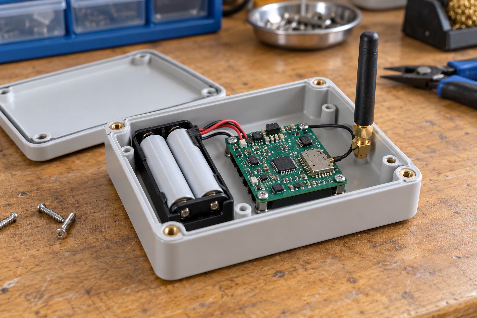
A soil-monitoring node combines the appropriate probe, conditioning or digital interface, a microcontroller, Wi-Fi or another supported radio, and a suitable power source. A Wi-Fi module provides network access; cloud connectivity additionally requires a working onward network and service.
Information chain: Soil sensor → readout/ADC → calibration and validity → microcontroller → Wi-Fi module/access point → network/cloud → dashboard. A digital probe may bypass a separate ADC channel but still needs data interpretation.
Attach time, location/channel identity, units and quality to measurements. Soil moisture, temperature and nutrient measurements have different sensing/calibration requirements. Raw conductivity is not a direct independent measurement of every NPK concentration.
Power management can reduce average consumption by sleeping between acquisitions and transmissions. Wake-up, sensor settling, conversion, connection and transmission all take time and energy. Connection overhead can dominate a short radio payload.
Field limitation: Water ingress, placement, soil conditions and network availability affect usefulness. A local irrigation decision can continue under a declared policy when cloud connectivity is unavailable; remote reporting and local control are separate functions.
Worked Problem 5.47: Soil-Node Average Current
Problem: A node draws 20 mA for 2 s and 0.2 mA for 58 s in each 60 s cycle. Find average current.
Model / approach: Time-weight both operating states.
Step 1: Charge-equivalent total = 20 × 2 + 0.2 × 58 = 51.6 mA·s.
Step 2: Iavg = 51.6/60.
Answer: 0.86 mA.
Check: Unlisted connection, sensor settling or regulator current would need to be added.
47. [C] Drone Electronics: ESC, BLDC and GPS
A drone combines sensing, flight-control computation, communication, power distribution and propulsion. The flight controller uses attitude/motion measurements and a control algorithm to command the propulsion stages; a GPS/GNSS receiver supplies navigation-related position/time information.
An electronic speed controller (ESC) uses power electronics to commutate and control a brushless DC (BLDC) motor. The flight controller sends a compatible command; the battery supplies motor power through the ESC. A GPIO command is not the motor-energy source.
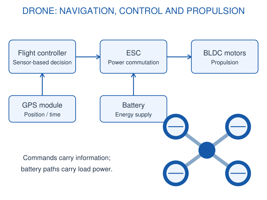
Navigation: A GPS module receives satellite signals to estimate position/time under suitable reception. It does not by itself maintain attitude, avoid every obstacle or replace inertial sensing. Antenna placement and signal availability matter.
Functional chain: Inertial/navigation sensors → flight controller → ESCs → BLDC motors; battery → distribution/ESC power paths. Telemetry carries status/commands through a separate communication function. Balance power budget, current demands, mass and required runtime at the stated operating point.
In precision agriculture a drone may carry a sensing payload for field observation. The electronics overview identifies roles and energy flow; it does not specify autonomous flight behaviour or a complete aircraft design.
Worked Problem 5.48: Drone Electrical Power
Problem: Four motors each draw a supplied 2 A at battery voltage 14.8 V. Electronics use another 1.6 W. Find total electrical power at this point.
Model / approach: Sum motor input power and the additional electronics load.
Step 1: Motor current = 4 × 2 = 8 A.
Step 2: Motor power = 14.8 × 8 = 118.4 W.
Step 3: Total = 118.4 + 1.6.
Answer: 120 W total electrical input power.
Check: Mechanical output and flight runtime require additional efficiency and energy information.
48. [C] Precision Agriculture: Irrigation and Greenhouse
Precision agriculture electronics combines calibrated measurements with targeted decisions and actuator control. Soil, temperature, humidity and light channels can support irrigation or greenhouse environmental management; the measurements must represent the relevant growing conditions.
An automated irrigation controller evaluates moisture and permitted operating conditions, then commands a suitable pump/valve driver. Hysteresis and time constraints can avoid rapid cycling. Invalid sensors, empty water supply and loss of communication require a defined response for the actual system.
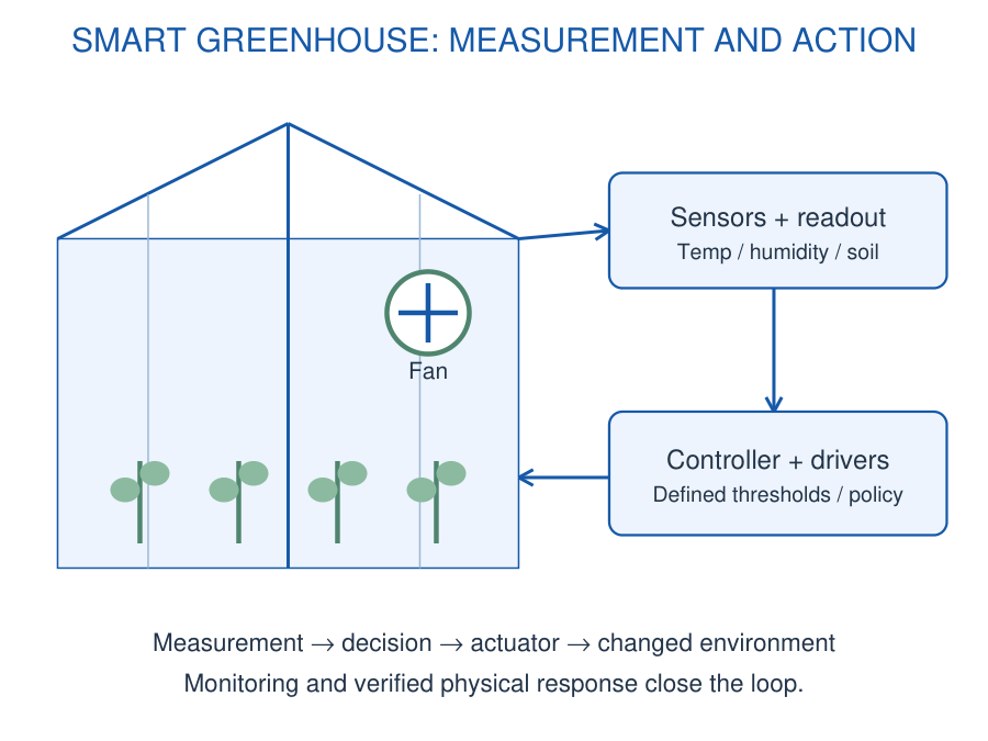
A smart greenhouse acquires temperature/humidity/light and possibly soil conditions, applies local decision logic and drives ventilation, irrigation, lighting or heating through rated interfaces. Data logging and remote dashboards support supervision while local decisions depend on their specified control policy.
Example logic: With permission E and conditions T for high temperature and H for high humidity, fan command F = E(T OR H) implements a declared rule. Numerical thresholds need calibration and a stated decision objective. More sensors do not automatically make a control policy suitable.
System check: Trace physical variable → calibrated signal → decision → driver → physical action → updated measurement. Feedback must reflect the action actually achieved. Distinguish a requested pump command from verified water flow.
Worked Problem 5.49: Greenhouse Fan Decision
Problem: Use F = E(T OR H). E is enable; T and H mean high temperature and high humidity. Evaluate (E,T,H) = (1,0,1), (0,1,1), (1,0,0).
Model / approach: Combine condition requests before applying permission.
Step 1: The OR results are 1,1,0.
Step 2: AND with E gives 1,0,0.
Answer: Fan commands 1,0,0.
Check: The truth table implements only the declared rule; thresholds and hysteresis are separate.
Worked Problem 5.50: Irrigation Volume
Problem: A verified constant flow is 2 L/min for an 8 min delivery interval. Find delivered volume.
Model / approach: Volume = flow rate × elapsed delivery time.
Step 1: V = 2 × 8.
Answer: 16 L.
Check: This assumes verified flow throughout; an electrical ON command alone does not prove the delivered amount.
49. FORMULAE AND SYSTEM REVISION
| Quantity | Expression and Stated Conditions |
|---|---|
| Ideal ADC step | q = Vref/2^N; ideal equal-width bin model |
| Counter first crossing | K = ceil(Vin/q); check representable range |
| Full flash comparators | 2^N – 1 for the stated conventional architecture |
| PWM timing | D = ton/T; f = 1/T |
| Unipolar resistive PWM | Vavg = DVS; Vrms = VS√D |
| Serial shift time | Time = total clocked/framed bits / bit rate |
| LDO loss estimate | P ≈ (Vin – Vout)Iout; add quiescent effects if given |
| Converter power | Pout = efficiency × Pin |
| Ideal energy runtime | t = usable energy / load power at matching boundary |
| Synchronous field speed | ns = 120f/P; not automatically rotor speed |
| Ultrasound depth | d = ct/2 for supplied uniform sound speed |
| Vibration RMS | √(mean of squared calibrated samples) |
System check: Establish signal range, conversion convention, timing, communication capacity and energy boundary before accepting a numerical result. A valid calculation for one block does not guarantee a functioning complete system.
| System Block | Its Role and Boundary |
|---|---|
| ADC | Codes a permitted voltage. Calibration supplies physical units. |
| PLC / SCADA | Local controller logic and supervisory acquisition have different roles. |
| VFD | Converts input power into controlled motor AC. |
| Biomedical readout | Sensing, conditioning and calibrated processing precede display. |
| Solar controller | Controls energy transfer using battery requirements and measurements. |
| ESC / GPS | Motor power commutation and navigation information are separate functions. |
Trace a missing measurement: A working network can still carry a flat, clipped or invalid value. Check the sensing element, excitation, conditioning range, ADC/reference, calibration and quality status before treating the display as a true physical reading.
Trace a missing action: An HMI command can be received without a load operating. Check local permissions, controller output state, driver compatibility, available load power and the feedback that confirms physical action. A requested ON state is not verified water flow or motor rotation.
Keep the calculation boundary: A correct average-current estimate says nothing by itself about radio coverage or sensor accuracy. A valid converter-efficiency model does not define a battery charge profile. Verify the conditions for every required block.
QUICK REVISION: EXPLAIN AND CHECK
What Does a Microcontroller Integrate?
A processor, memory and peripherals such as GPIO, timers, conversion and communication functions, depending on the device.
Why Separate Supply and Reference?
A supply powers a block; the ADC reference establishes the conversion scale. They may be related but are not automatically identical.
How Does Counter-Ramp Conversion Differ from Flash?
A counter repeatedly increases a DAC level; a conventional flash uses many simultaneous comparisons and an encoder.
Is PWM a Continuously Adjustable Analog Voltage?
It is a pulse waveform with controlled timing. An average or filtered response requires a stated load or filter model.
What Distinguishes UART, SPI and I2C?
UART uses agreed asynchronous framing; SPI uses clocked selected transfers; I2C shares addressed data/clock lines with appropriate pull-ups.
Does Wi-Fi Ensure Cloud Access?
No. Association with a local network and a working onward service connection are separate conditions.
Why Can an LDO Dissipate Significant Heat?
The voltage difference multiplied by load current is largely dissipated in the linear regulating path.
What Does a BMS Monitor?
Cell/pack conditions such as voltage, current and temperature to support protection, balancing and state estimation.
What Does a PLC Do?
It acquires field inputs, executes control logic and updates suitable output interfaces.
What Are the VFD Power Stages?
Rectifier, DC bus and inverter. A controller commands switching separately from the motor-energy path.
How Do SCADA and HMI Differ?
SCADA is a supervisory acquisition/control system; an HMI is the operator-facing interface, which may also be a local panel.
Does Vibration Growth Prove One Fault?
No. Compare calibrated trends at stated mounting and operating conditions before attributing a cause.
What Is Shared by Biomedical Readout Chains?
Sensing, appropriate conditioning, acquisition, calibrated processing and meaningful display, with complete instrument requirements.
Why Divide Ultrasound Travel Distance by Two?
Echo time includes outward and return travel in the stated pulse-echo model.
What Do ESC and GPS Do on a Drone?
An ESC controls motor commutation/power; GPS supplies navigation-related position/time information.
What Closes an Agricultural Control Loop?
A physical action changes the measured condition. Verify achieved flow or environmental response rather than equating a command with success.
| Path | Main Question | Evidence Needed |
|---|---|---|
| Information | Is the value meaningful? | Calibration, timing and quality |
| Control | Is the decision correct? | Input meaning, logic and state |
| Energy | Can the load act? | Supply, driver and power limits |