
AKTU B.TECH 1ST YEAR | SEMESTER I & II
COURSE CODES: AEC101A / AEC201A | AEC101B / AEC201B | AEC101C / AEC201C
UNIT I – Diodes, Rectifiers, Power Supplies and Photodetectors
Common to CSE, EE, ECE, CE, ME, CH, TX, BT & AG Streams
Unit I Introduction
Diodes, Rectifiers and Power Supplies develops the p-n junction, diode models, rectification, reservoir filtering, Zener regulation, LED current control and photodetectors. Worked examples connect the principles with board supplies, PLCs, optical sensing, diagnostic instruments and greenhouse monitoring.
Topic Map
| Topic | Pages |
|---|---|
| Junction, bias, models and diode circuits | 3–11 |
| Half-wave and bridge rectification | 11–18 |
| Capacitor filters, ripple and ratings | 18–22 |
| Zener regulation and design | 22–26 |
| LEDs, resistors and strings | 26–28 |
| Board supplies and USB charger | 28–31 |
| Photodetectors and industrial applications | 31–33 |
| Biomedical and agriculture applications | 33–34 |
| Formulae, tricks and revision | 34–35 |
Coverage
All A, B and C code pairs across nine streams. Page 2 gives the branch-wise topic map and official unit names. Follow the common foundation and the sections prescribed for your group.
How to Use These Notes
- Read the principle and labelled diagram before the calculations.
- Mark A/K terminals, current directions and voltage references.
- State the ideal, constant-drop or supplied linear diode model.
- Try each worked problem before reading its solution.
- Check the circuit state and physical meaning after calculating.
- Use each formula together with its stated assumptions.
What Is Included?
| Study support | Included |
|---|---|
| Worked problems | 50, with calculation steps and interpretation |
| Circuit diagrams and plots | 35 circuit and application figures |
| Realistic images | 10 component and laboratory images |
| Exam shortcuts | Conditions, memory cues and common traps |
| Applications | Board supplies, PLCs, optical sensing and biomedical/agri systems |
| End revision | Formula sheet and short-answer review |
Numerical Convention
Values are educational assumptions. Retain precision until the final answer. Ground is a voltage reference; terminals need not all be positive.
Main Idea
Choose the circuit model, trace the current path, calculate and verify. Check the waveform and assumed diode state before applying a formula.
Unit Overview and Branch-Wise Reading Map
One combined unit covers the shared diode and power-supply foundation, followed by the additional applications for each syllabus group. Use the branch map below to choose the prescribed sections after reading the shared topics. A, B and C refer to the code suffixes in this subject.
| Topics / application block | Applicable branches | Where to read |
|---|---|---|
| PN junction, bias, rectifiers, capacitor filter, Zener regulation and LED working / current limiting | All nine streams | Sections 1–36 |
| Ideal/real models and detailed V-I (A); diode switching (A & B) | A: CSE, EE, ECE; B: CE, ME, CH, TX for switching | Sections 6–12; enrichment for C |
| 5 V / 3.3 V board supplies, USB charger rectification and LED indicators | A: CSE, EE, ECE | Sections 33–39 |
| Photodiode function | B: CE, ME, CH, TX; C: BT, AG | Section 41 |
| PLC/control-panel supply, machinery indicators, conveyor sensing, field-instrument supply | B: CE, ME, CH, TX | Sections 42–43 |
| Phototransistor function | C: BT, AG | Section 41 |
| pH meter/glucometer supply, diagnostic LEDs, pulse oximeter, greenhouse light sensor | C: BT, AG | Sections 44–45 |
| Worked problems, diagnosis, formulae and revision | All streams: choose the relevant application | Throughout; Sections 40, 46–48 |
Syllabus Groups and Official Unit Names
- A – CSE, EE, ECE: Diodes and Power Supply Circuits.
- B – CE, ME, CH, TX: Diodes, Rectifiers, and Regulated Power Supplies.
- C – BT, AG: Diodes, Power Supply, and LED Circuits.
What Is Included
50 numbered worked problems with calculation steps and checks; 10 realistic component/laboratory images; labelled circuit diagrams and photodetector application diagrams. The two semester codes in each group use the same unit syllabus.
Study approach: Trace the current path, state the diode model, calculate and verify the assumed state. A coloured [B] or [C] section label identifies additional group-specific coverage. Values in problems are stated educational assumptions.
1. THE COMPLETE POWER-SUPPLY PICTURE
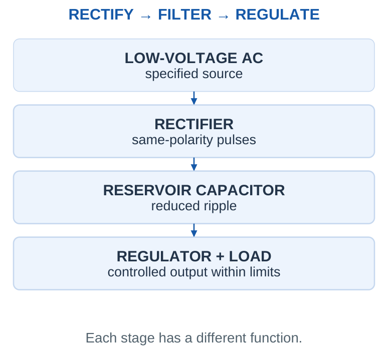
A supply circuit changes the available electrical source into a form suitable for its load. A rectifier produces unidirectional output, a reservoir capacitor reduces the voltage change between charging pulses, and a regulator controls the output over a specified operating range. These stages do different jobs. A rectifier alone does not produce a perfectly steady 5 V output.
The diode is the central device in this unit. Its asymmetric current-voltage behaviour permits rectification and switching. A Zener diode uses controlled reverse breakdown for a voltage reference or low-power shunt regulation. An LED converts part of its electrical input into emitted light and needs a controlled current.
| Circuit | Main question |
|---|---|
| Ordinary diode | Is it forward conducting or blocking? |
| Rectifier | Which path carries each half-cycle? |
| Filter | How far does voltage fall between recharges? |
| Zener regulator | Is current inside the regulation window? |
| LED indicator | What limits LED current? |
Study route
Learn the device model first, then trace the circuit, calculate, and verify the assumed state. This order is faster and more reliable than searching for a formula before identifying the circuit.
2. SEMICONDUCTORS, CARRIERS AND DOPING
Silicon forms a bonded crystal structure. An electron promoted into a mobile state can carry charge; the missing electron in a bond is represented as a hole. An intrinsic semiconductor has thermally generated electron-hole pairs. Doping introduces controlled impurity atoms that alter carrier populations without turning the material into a net charged block. In n-type material, electrons are majority carriers and holes are minority carriers. In p-type material, holes are majority carriers and electrons are minority carriers. The labels p and n describe carrier type; they do not mean an isolated sample must have a large net positive or negative charge.
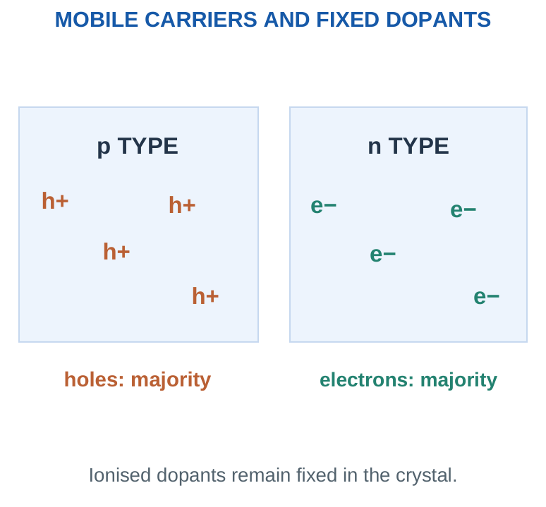
Diffusion is carrier movement associated with a concentration gradient. Drift is carrier motion associated with an electric field. Conventional current follows the direction of positive charge movement; electron motion contributes current in the opposite direction to its own velocity.
Memory trick
n → negative mobile electrons; p → positive mobile holes. Keep this separate from the charge of the fixed dopant ions after ionisation.
3. FORMATION OF THE p-n JUNCTION
When p-type and n-type regions form a junction, electrons and holes diffuse toward regions where their concentrations are lower. Recombination near the junction leaves a region depleted of many mobile majority carriers. Fixed ionised acceptors remain on the p side and fixed ionised donors remain on the n side. The resulting electric field points from the positive donor-ion region toward the negative acceptor-ion region: from n toward p in the illustrated orientation. This field opposes further majority-carrier diffusion. At thermal equilibrium, drift and diffusion currents balance so that the net terminal current is zero.
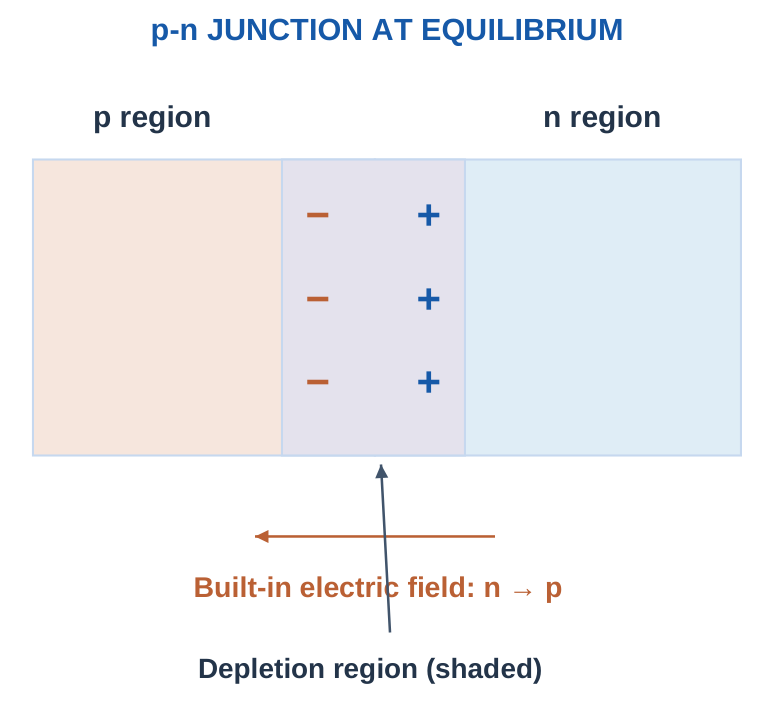
The depletion region is not empty of atoms and is not a literal air gap. Its name refers to the reduced mobile-carrier concentration relative to the neutral regions. The built-in barrier also should not be treated as a freely available battery voltage measurable across an isolated diode with an ordinary voltmeter.
Exam answer
Explain diffusion → recombination → exposed fixed ions → electric field → equilibrium. A labelled sketch of the ions and field is more useful than writing only “a barrier is formed.”
4. FORWARD AND REVERSE BIAS
A diode has an anode A and cathode K. For the ordinary p-n junction, A corresponds to the p side and K to the n side. Define diode voltage as vD = vA – vK and positive diode current from A to K. Always state this reference before interpreting signs. Forward bias connects the p side toward the positive terminal relative to the n side. It lowers the junction barrier and generally narrows the depletion region, allowing substantial carrier injection and forward current. Reverse bias raises the barrier and generally widens the depletion region; a small reverse leakage current can exist before breakdown.
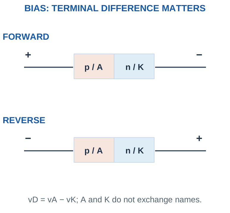
A cathode at 4 V and an anode at 2 V give vD = -2 V. The diode is reverse biased even though both nodes are positive relative to ground. Bias depends on the difference between terminals, not whether either terminal is individually above zero.
Fast check
Subtract A – K. Positive favours forward bias; negative indicates reverse bias. Then apply the stated diode model to decide the current, including the external current-limiting path.
Worked problem 1.1: Terminals 5 V and 1 V
Problem. The anode is at 5 V and cathode at 1 V relative to the same ground. Find vD and identify the applied bias.
Model / approach. Use vD = vA – vK; no current is calculated without the external circuit.
Step 1. Keep the anode first: vD = 5 – (1) = 4 V.
Step 2. The sign corresponds to forward bias under the chosen reference.
Answer: vD = 4 V; forward bias.
Check and interpretation. Changing the ground reference equally at both terminals leaves the voltage difference unchanged. Forward bias by itself does not set a unique current; the source and limiting impedance are still needed.
Worked problem 1.2: Terminals 2 V and 4 V
Problem. The anode is at 2 V and cathode at 4 V relative to the same ground. Find vD and identify the applied bias.
Model / approach. Use vD = vA – vK; no current is calculated without the external circuit.
Step 1. Keep the anode first: vD = 2 – (4) = -2 V.
Step 2. The sign corresponds to reverse bias under the chosen reference.
Answer: vD = -2 V; reverse bias.
Check and interpretation. Changing the ground reference equally at both terminals leaves the voltage difference unchanged. Forward bias by itself does not set a unique current; the source and limiting impedance are still needed.
Worked problem 1.3: Terminals -1 V and -4 V
Problem. The anode is at -1 V and cathode at -4 V relative to the same ground. Find vD and identify the applied bias.
Model / approach. Use vD = vA – vK; no current is calculated without the external circuit.
Step 1. Keep the anode first: vD = -1 – (-4) = 3 V.
Step 2. The sign corresponds to forward bias under the chosen reference.
Answer: vD = 3 V; forward bias.
Check and interpretation. Changing the ground reference equally at both terminals leaves the voltage difference unchanged. Forward bias by itself does not set a unique current; the source and limiting impedance are still needed.
5. SYMBOLS, POLARITY AND MEASUREMENT
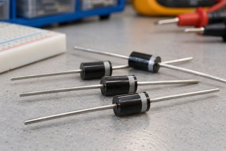
Component view 1. Axial rectifier diodes: the body band identifies the cathode terminal.
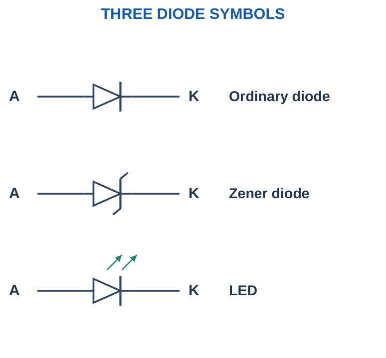
The bar in a standard diode symbol identifies the cathode. Many axial rectifier packages also mark the cathode with a band; confirm the actual component documentation. A bridge package has two AC terminals and DC +/- terminals, so it should not be connected by guessing from its outer shape.
A multimeter diode-test mode applies a small test current and displays a voltage-related reading when the polarity and device permit conduction. A reverse reading may show an open indication. An in-circuit reading can be affected by parallel paths, and a displayed number is not a complete characteristic curve or proof of every rating.
| Observation | Interpretation |
|---|---|
| A-to-K test conducts; reversed test blocks | Consistent with an ordinary working diode under that test |
| Low reading in both directions | Could indicate a short or parallel circuit path |
| Open in both directions | Could indicate an open device, unsuitable test conditions or an LED beyond tester compliance |
Practical habit
Use the symbol and the datasheet together. A package marking identifies a terminal; it does not specify forward voltage at every current or the permitted reverse stress.
6. DIODE V-I CHARACTERISTIC
The forward characteristic is nonlinear: current rises rapidly as forward voltage increases over an operating region. A real silicon diode does not have a perfectly fixed 0.7 V threshold followed by unlimited current. Its forward drop depends on current, temperature and construction. A constant 0.7 V is a useful stated calculation model, not a universal material constant.
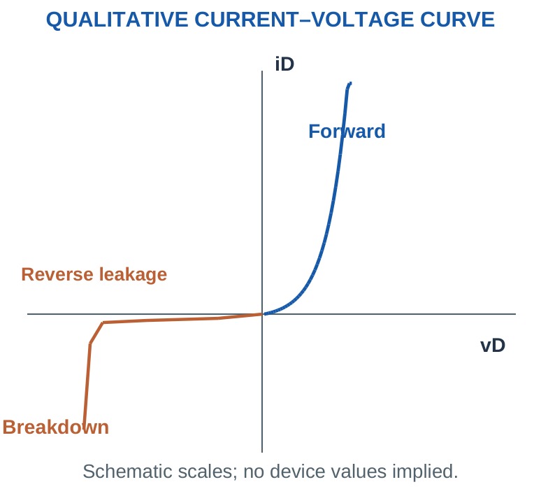
Reverse current is small below breakdown under suitable conditions, but not exactly zero in a real device. Ordinary rectifiers are normally selected to block the intended reverse voltage; a Zener diode is specifically used in a controlled reverse-breakdown circuit. External current limitation and dissipation remain essential. A plotted curve must identify voltage polarity, current direction, units and scale. Forward amperes and reverse microamperes may be shown at different scales. Do not infer equal forward and reverse current magnitudes merely because two branches occupy similar visual space.
Trick with a condition
Use 0.7 V only when the question explicitly gives it or accepts the silicon constant-drop approximation. If a datasheet or measured curve gives a different value at the operating current, use that value.
7. IDEAL, CONSTANT-DROP AND LINEAR MODELS
An ideal diode is a short circuit in its permitted forward-conducting state and an open circuit in its blocking state. It has zero forward drop and no reverse leakage in that model. A constant-drop model replaces the conducting diode by a fixed forward drop VF, while retaining an open blocking state before breakdown.
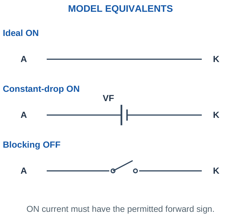
A piecewise-linear model can add a forward resistance rd after a threshold V0: vD = V0 + iD rd in the assumed ON region. It is useful when supplied in a problem, but does not reproduce every temperature, switching or breakdown effect.
| Model | ON relation | OFF simplification |
|---|---|---|
| Ideal | vD = 0, iD ≥ 0 | iD = 0, vD ≤ 0 |
| Constant drop | vD = VF, iD ≥ 0 | No forward conduction below the assumed threshold |
| Piecewise linear | vD = V0 + iD rd | Blocking branch as specified |
Model discipline
Do not use an ideal diode for the current calculation and then subtract 0.7 V again in the same loop. Select one model and apply it consistently.
8. ASSUME, SOLVE AND VERIFY THE STATE
For a simple diode circuit, first assume a conducting or blocking state. Replace the diode by the correct equivalent, solve the resulting linear circuit and check whether the calculated terminal values support the assumption. A contradictory assumption must be rejected and the alternative tested.
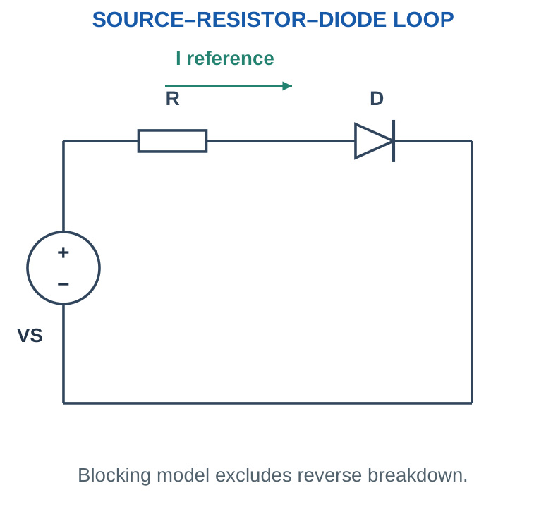
For a forward series loop under the constant-drop model, I = (VS – VF)/R only if that gives a valid nonnegative conducting current. If the source cannot forward-bias the diode in the stated circuit, use the blocking solution rather than reporting a negative forward current through a one-way ideal device. For an OFF diode, solve node voltages with its branch open and calculate vA – vK. An open circuit means zero branch current; it does not require zero voltage across the device. A short circuit means zero voltage in the ideal model; it does not require zero current.
Four-step answer
- Mark A/K.
- State the model and assumed state.
- Solve KVL/KCL.
- Check current sign or terminal voltage.
Include the final state with the numerical answer.
Worked problem 1.4: Series source 5 V
Problem. A forward-oriented diode and 1000 Ω resistor are in series with a 5 V source. Use VF = 0.7 V. Find current and resistor voltage.
Model / approach. Assume the diode is ON in the stated constant-drop model; VF = 0 represents the ideal model.
Step 1. VR = VS – VF = 5 – 0.7 = 4.3 V.
Step 2. I = VR/R = 4.3/1000 = 0.0043 A = 4.3 mA.
Answer: I = 4.3 mA; VR = 4.3 V.
Check and interpretation. The positive calculated current supports the forward-conducting assumption. The resistor prevents an unlimited ideal-source current. A different current-dependent diode curve can change the actual operating point.
Worked problem 1.5: Series source 12 V
Problem. A forward-oriented diode and 2200 Ω resistor are in series with a 12 V source. Use VF = 0.7 V. Find current and resistor voltage.
Model / approach. Assume the diode is ON in the stated constant-drop model; VF = 0 represents the ideal model.
Step 1. VR = VS – VF = 12 – 0.7 = 11.3 V.
Step 2. I = VR/R = 11.3/2200 = 0.0051364 A = 5.1364 mA.
Answer: I = 5.1364 mA; VR = 11.3 V.
Check and interpretation. The positive calculated current supports the forward-conducting assumption. The resistor prevents an unlimited ideal-source current. A different current-dependent diode curve can change the actual operating point.
Worked problem 1.6: Series source 3.3 V
Problem. A forward-oriented diode and 470 Ω resistor are in series with a 3.3 V source. Use VF = 0.6 V. Find current and resistor voltage.
Model / approach. Assume the diode is ON in the stated constant-drop model; VF = 0 represents the ideal model.
Step 1. VR = VS – VF = 3.3 – 0.6 = 2.7 V.
Step 2. I = VR/R = 2.7/470 = 0.0057447 A = 5.7447 mA.
Answer: I = 5.7447 mA; VR = 2.7 V.
Check and interpretation. The positive calculated current supports the forward-conducting assumption. The resistor prevents an unlimited ideal-source current. A different current-dependent diode curve can change the actual operating point.
Worked problem 1.7: Below the assumed threshold
Problem. A 0.4 V source drives a forward-oriented diode through 1 kΩ. The model has an ON drop of 0.7 V and a blocking OFF branch. Determine current.
Model / approach. Test the ON assumption, then reject it if its current has the wrong sign.
Step 1. Assumed ON current = (0.4 – 0.7)/1,000 = -0.0003 A. This contradicts the allowed forward direction.
Step 2. Use OFF: I = 0. Resistor drop is zero, so the diode sees 0.4 V, below the assumed threshold.
Answer: OFF; I = 0 in this model.
Check and interpretation. A real diode can carry a small forward current below 0.7 V. The zero answer belongs to the specified piecewise model, not an assertion that semiconductor current is physically zero below one exact voltage.
9. BLOCKING, REVERSED SOURCES AND TWO DIODES
A reverse-biased diode can interrupt a series path under the ideal or pre-breakdown constant-drop model. The resistor then has no voltage drop if its current is zero, so the external source can appear across the diode. This is why checking reverse voltage is a separate part of a diode problem.
Two series diodes oriented in the same direction require the sum of their assumed forward drops. Two ordinary diodes oriented in opposite series directions block steady current in the ideal pre-breakdown model for either source polarity. That statement excludes reverse breakdown and capacitive or switching transients.
Counting trick
Count only the diodes in the actual conducting loop. A four-diode bridge has four devices in its drawing but normally only two in a resistive-load conduction path at a time.
Worked problem 1.8: Reverse-oriented series diode
Problem. A 9 V DC source, 1000 Ω resistor and reverse-oriented ordinary diode form a loop. Ignore leakage and breakdown. Find current, resistor drop and diode reverse-voltage magnitude.
Model / approach. Open-circuit the blocking diode branch.
Step 1. I = 0 because the permitted forward path is absent.
Step 2. VR = IR = 0. KVL therefore places the source voltage across the diode in reverse.
Answer: I = 0; VR = 0; reverse magnitude = 9 V.
Check and interpretation. No resistor drop does not imply no voltage anywhere. The open diode can support a voltage while current is zero. The result would require another model if reverse breakdown or leakage were explicitly included.
Worked problem 1.9: 2 forward diodes in series
Problem. A 5 V source drives 2 same-direction series diodes and 1000 Ω. The diode drops are 0.7 V, 0.7 V. Find the loop current.
Model / approach. All diodes are assumed ON; add the drops in the one conducting loop.
Step 1. Combined forward drop = 1.4 V.
Step 2. I = (5 – 1.4)/1000 = 3.6 mA.
Answer: Forward current = 3.6 mA.
Check and interpretation. The same current passes through every element in this series path. Positive current verifies the assumption for this simplified model. Do not divide the current by the number of diodes.
10. LOAD LINE AND OPERATING POINT
For a source VS, series resistor R and diode, KVL gives iD = (VS – vD)/R. This straight line is the circuit load line. Its intercepts are iD = VS/R at vD = 0 and vD = VS at iD = 0. The operating point lies where this line intersects the diode characteristic.
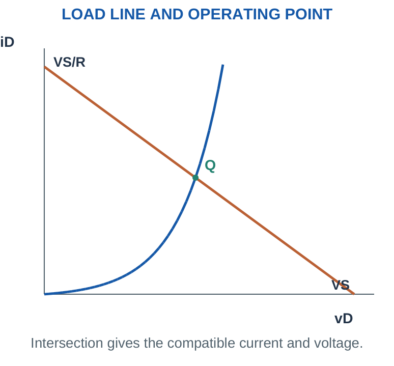
Increasing R makes the current intercept smaller for a fixed source. Changing VS shifts the line. A supplied piecewise-linear device model can be substituted into KVL to solve algebraically: I = (VS – V0)/(R + rd). Keep the resistance inside the diode model separate from the external resistor. Static resistance VD/ID describes a ratio at a point. Small-signal or dynamic resistance ΔVD/ΔID describes a local slope. These are generally different for a nonlinear curve. This unit uses them only where a problem supplies the necessary data; a full semiconductor equation derivation is not required.
Graph trick
Mark both intercepts before drawing the load line. An attractive line with the wrong current intercept gives the wrong operating point even if the diode curve looks plausible.
LOAD-LINE CHECKPOINTS
At vD = 0: iD = VS/R. At iD = 0: vD = VS. Both intercepts must use the same reference directions.
Worked problem 1.10: Piecewise-linear operating point
Problem. VS = 5 V, external R = 1000 Ω. The conducting diode model is vD = 0.6 + iD(20 Ω). Find iD and vD.
Model / approach. Use KVL with the supplied forward resistance; current is in amperes.
Step 1. VS = I R + V0 + I rd, so I = (5 – 0.6)/(1000 + 20) = 0.0043137 A.
Step 2. vD = 0.6 + 20 × 0.0043137 ≈ 0.6863 V.
Answer: I ≈ 4.3137 mA; vD ≈ 0.6863 V.
Check and interpretation. Using the unrounded current, the external resistor and diode drops add back to the source. This local linear model is only being used in its specified conducting region.
Worked problem 1.11: Static and dynamic resistance
Problem. At one point a diode has VD = 0.72 V and ID = 12 mA. A nearby increase of 2 mA produces a 10 mV rise. Find static resistance and local dynamic resistance.
Model / approach. Use a point ratio for static resistance and a change ratio for dynamic resistance.
Step 1. Rstatic = 0.72/0.012 = 60 Ω.
Step 2. rd ≈ 0.010/0.002 = 5 Ω.
Answer: 60 Ω static; 5 Ω dynamic.
Check and interpretation. The two values differ because the diode characteristic is nonlinear. Dynamic resistance describes the local slope; it is not automatically the total diode voltage divided by its DC current.
11. POWER, RATINGS AND WORST CASES
POWER BALANCE IN A DC LOOP
For one conducting diode and a series resistor:
Pin = VS I
PR = I²R; PD = VF I
Pin = PR + PD
Use the same operating current throughout. A power rating must exceed the relevant operating dissipation under its specified conditions.
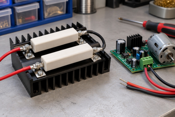
Component view 2. Power components and heat sinks: thermal design is part of the component rating.
Diode forward dissipation in the constant-drop steady model is approximately PD = VF I. Series-resistor dissipation is PR = I²R = VR I = VR²/R. The source supplies VS I in the simple loop, and the dissipations should add to the input power when those are the only elements storing or consuming energy. A resistor’s nominal ohmic value and power rating answer different questions. A current calculation gives the working dissipation; a practical rating must also account for temperature and derating conditions. A maximum datasheet rating is a limit under stated conditions, not a recommendation to operate exactly at that limit indefinitely.
Worst-case current usually uses maximum source voltage, minimum forward drop and minimum resistance in a resistively limited forward branch. For a blocked rectifier, reverse-voltage stress is evaluated separately. A capacitor input can create short charging pulses and startup surge, so DC load current alone does not specify peak diode current.
Sanity check
Calculate both voltage and power. A resistor can have the right resistance but an inadequate power rating. A diode can have enough current capability but insufficient reverse-voltage capability.
Worked problem 1.12: Account for every watt
Problem. A 12 V source feeds a diode of assumed drop 0.7 V through 1000 Ω. Find source power, resistor power and diode power.
Model / approach. Steady constant-drop loop; no energy-storage element is present.
Step 1. I = (12 – 0.7)/1000 = 11.3 mA.
Step 2. PR = I²R ≈ 0.1277 W; PD = VF I ≈ 0.0079 W.
Step 3. Pin = VS I ≈ 0.1356 W. Check PR + PD = Pin with unrounded values.
Answer: PR ≈ 127.69 mW; PD ≈ 7.91 mW.
Check and interpretation. The power sum checks both arithmetic and the circuit boundary. A practical resistor or diode rating also needs the relevant thermal conditions; this exercise computes operating dissipation.
Worked problem 1.13: Source and resistance tolerances
Problem. A source varies from 4.75 to 5.25 V; diode VF is assumed 0.6–0.8 V; R = 470 Ω ±5%. Find maximum and minimum branch current under this constant-drop model.
Model / approach. Use all three extremes in the direction that produces the required current corner.
Step 1. Rmin = 470 × 0.95 = 446.5 Ω; Rmax = 493.5 Ω.
Step 2. Imax = (5.25 – 0.6)/446.5 ≈ 10.4143 mA.
Step 3. Imin = (4.75 – 0.8)/493.5 ≈ 8.0041 mA.
Answer: Approximate current range: 8.0041–10.4143 mA.
Check and interpretation. The nominal current alone would miss the extremes. The assumed VF range must be applicable to the relevant operating conditions; real forward voltage and current are related rather than fully independent parameters.
12. DIODE AS AN ELECTRONIC SWITCH
A diode changes its conduction state according to its terminal conditions rather than a separate gate command. In the ideal model, forward conduction behaves like a closed switch and blocking like an open switch. The real device has a forward drop, leakage, capacitance and finite switching behaviour.
A simple diode can steer signals or provide polarity-dependent connection. It is not a bidirectional mechanical switch, and it cannot isolate every possible direction of energy flow under all conditions. Reverse recovery matters in switching applications but is introduced here only as a real-device limitation, not a detailed switching-design topic.
Exam phrasing
Write “approximately closed in forward conduction” and “approximately open before reverse breakdown” when describing a real device. Then state the ideal simplification used for the calculation.
Worked problem 1.14: Ideal switch state from input
Problem. The source voltage in a positive half-wave-oriented diode/resistor loop is instantaneously 4 V and R = 2000 Ω. Use an ideal diode. Find state and current.
Model / approach. Apply the permitted A-to-K current direction for this source polarity.
Step 1. For this orientation, output = max(4, 0) = 4 V.
Step 2. I = Vout/R = 4/2000 = 2 mA.
Answer: Conducting; I = 2 mA.
Check and interpretation. At exactly zero voltage and current, ideal ON/OFF state labels can be nonunique while the circuit quantities agree. For nonzero source values, verify the current sign or reverse-voltage condition.
13. AC QUANTITIES BEFORE RECTIFICATION
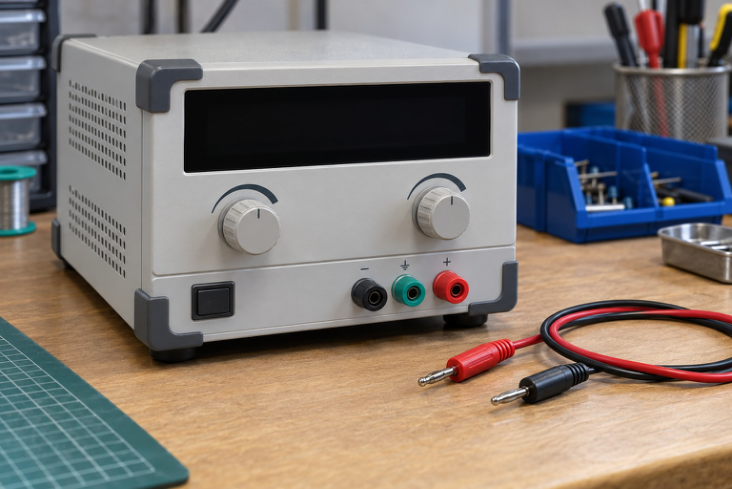
Component view 3. A laboratory DC supply provides a stated output voltage and current limit.
For a sinusoid v(t) = Vm sin(2πft), Vm is peak amplitude and f is frequency in hertz. The period is T = 1/f. For that sinusoid, RMS voltage is Vm/√2 and peak-to-peak voltage is 2Vm. These relationships do not apply unchanged to every nonsinusoidal waveform.
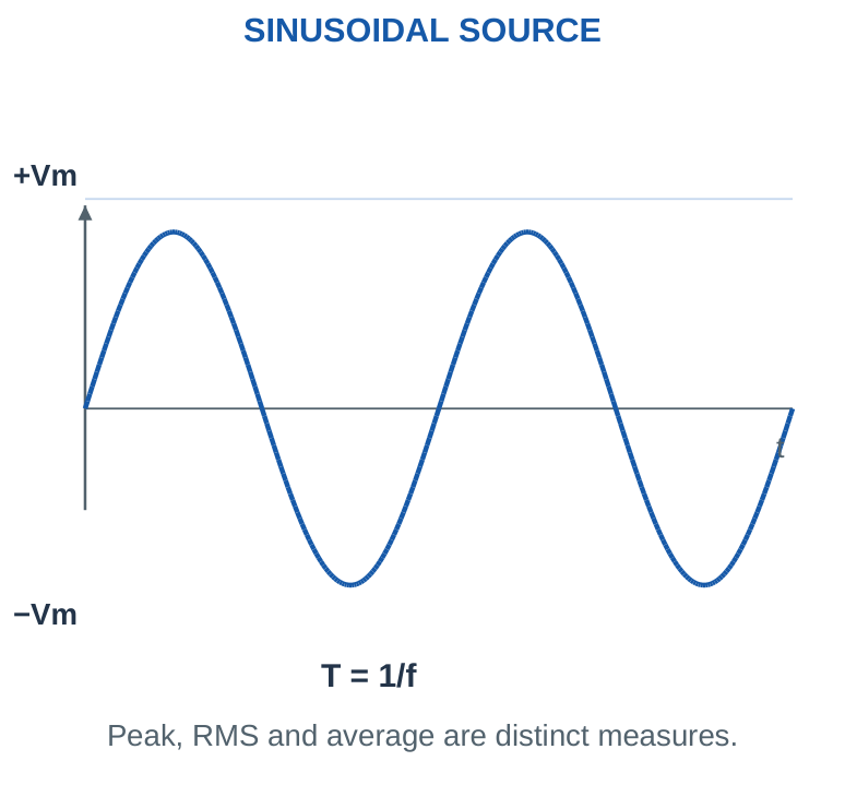
A transformer secondary specified as 12 V RMS has an ideal sinusoidal peak near 16.97 V. It does not have a peak of 12 V. A capacitor after a rectifier charges toward a peak-related voltage under suitable conditions, which explains why the DC reservoir can be higher than the input RMS number. The full-cycle average of a symmetric unrectified sine wave is zero, but its RMS is not zero. After rectification, the average becomes positive for the illustrated polarity. Use the intended waveform before choosing average or RMS formulae.
Three labels
Peak Vm, RMS Vrms, average VDC. Keep all three in your working. The letter “AC” on a source is not enough to tell whether a quoted number is peak or RMS; read the question.
Worked problem 1.15: RMS, peak, peak-to-peak and period
Problem. A sinusoidal source is 12 V RMS at 50 Hz. Find peak, peak-to-peak voltage and period.
Model / approach. Use sinusoidal relations; these values describe the source before rectification.
Step 1. Vm = √2 × 12 ≈ 16.9706 V.
Step 2. Vpp = 2Vm ≈ 33.9411 V.
Step 3. T = 1/50 s ≈ 20 ms.
Answer: Vm ≈ 16.9706 V; Vpp ≈ 33.9411 V; T ≈ 20 ms.
Check and interpretation. Peak-to-peak is measured from negative peak to positive peak. The average over a complete symmetric unrectified cycle is zero, although the RMS is the nonzero value supplied.
Worked problem 1.16: Instantaneous value
Problem. A 10 V-peak sine has v = 10 sin θ. Find v at θ = 30°, 90° and 210°.
Model / approach. The angles are electrical phase angles in degrees.
Step 1. v(30°) = 10 × 0.5 = 5 V.
Step 2. v(90°) = 10 V; v(210°) = 10 × (-0.5) = -5 V.
Answer: 5 V, 10 V and -5 V.
Check and interpretation. The negative value indicates polarity relative to the chosen source reference. A positive half-wave diode would block the last instant in the ideal model, giving zero positive-load output there.
14. HALF-WAVE RECTIFIER: CIRCUIT AND STATES
A positive half-wave rectifier uses a diode and load so that the positive input half-cycle produces positive load current. During the negative half-cycle, the diode blocks under the pre-breakdown ideal model. The output is pulsating DC: one polarity, varying magnitude.
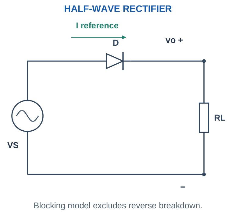
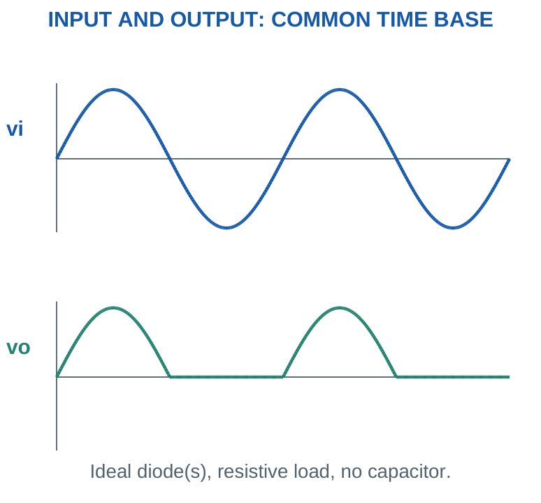
For an ideal diode and resistive load, vo = max(vi, 0). The current waveform is io = vo/RL. For a constant forward drop, vo = max(vi – VF, 0), so conduction begins only when the input exceeds the assumed drop. Reversing the diode reverses the selected output polarity in the appropriate loop.
Path trick
Start at the instantaneously positive source terminal, follow forward-oriented devices through the load, and return to the other terminal. If no complete permitted loop exists, the ideal load current is zero.
Worked problem 1.17: Instantaneous half-wave output
Problem. At one instant vi = 8 V. A positive HWR has VF = 0.7 V and RL = 1000 Ω. Find vo and io.
Model / approach. Use vo = max(vi – VF, 0) for the stated constant-drop resistive-load circuit.
Step 1. vi – VF = 8 – 0.7 = 7.3 V.
Step 2. After applying the blocking condition, vo = 7.3 V and io = vo/1000 = 7.3 mA.
Answer: vo = 7.3 V; io = 7.3 mA.
Check and interpretation. A negative algebraic forward-output result is replaced by the OFF solution rather than reported as negative current through the positive rectifier path. No filter capacitor is present.
Worked problem 1.18: Instantaneous half-wave output
Problem. At one instant vi = -8 V. A positive HWR has VF = 0.7 V and RL = 1000 Ω. Find vo and io.
Model / approach. Use vo = max(vi – VF, 0) for the stated constant-drop resistive-load circuit.
Step 1. vi – VF = -8 – 0.7 = -8.7 V.
Step 2. After applying the blocking condition, vo = 0 V and io = vo/1000 = 0 mA.
Answer: vo = 0 V; io = 0 mA.
Check and interpretation. A negative algebraic forward-output result is replaced by the OFF solution rather than reported as negative current through the positive rectifier path. No filter capacitor is present.
15. HALF-WAVE AVERAGE, RMS AND POWER
For a sinusoidal source, ideal diode, no filter and resistive load: VDC = Vm/π; Vrms = Vm/2; IDC = Im/π; Irms = Im/2; and Im = Vm/RL. The RMS includes both the DC component and the ripple component. It is not equal to the RMS ripple alone.
The DC-component load power is PDC = VDC²/RL. Total load heating power is Pac+dc = Vrms²/RL. The conventional rectification efficiency for the ideal half-wave resistive-load model is their ratio: 4/π² ≈ 40.5%. Textbooks often quote about 40.6% after rounding.
Important distinction
The conventional rectification efficiency measures useful DC-component power relative to total rectifier input in the stated model. It is not the same as saying an ideal zero-drop diode dissipates the remaining 59.5% as heat. The load still absorbs the ripple-related part of its total power.
These simple formulae are not the capacitor-filter output formulae. A filtered supply often sits near the rectified peak with a small droop, so Vm/π would give the wrong average for that different waveform.
USE THE CORRECT RMS
Load heating: Ptotal = Vrms,total²/RL. DC-component power: PDC = VDC²/RL. These are different when ripple is present.
Worked problem 1.19: Complete ideal half-wave calculation
Problem. An ideal unfiltered HWR has Vm = 20 V and RL = 1000 Ω. Find VDC, total Vrms, IDC, Irms and DC-component load power.
Model / approach. Sinusoidal input, ideal diode and resistive load; use the no-filter formula set.
Step 1. VDC = 20/π ≈ 6.3662 V; Vrms = 20/2 = 10 V.
Step 2. IDC = VDC/RL ≈ 6.3662 mA; Irms = Vrms/RL = 10 mA.
Step 3. PDC = VDC²/RL ≈ 0.0405 W; total load heating = Vrms²/RL = 0.1 W.
Answer: VDC ≈ 6.3662 V; total RMS = 10 V.
Check and interpretation. The DC-component power is smaller than total heating power because the output includes ripple. This does not imply an ideal zero-drop diode dissipates the difference.
16. HALF-WAVE RIPPLE, FREQUENCY AND PIV
Define ripple factor r = Vr,ac,rms/VDC, where Vr,ac,rms is the RMS of only the AC component. With total output RMS Vrms, use r = √[(Vrms/VDC)² – 1]. For the ideal unfiltered half-wave sine, r = √(π²/4 – 1) ≈ 1.211, or 121.1%. Do not confuse a dimensionless ratio with its percentage. A half-wave output has one pulse per source cycle, so its fundamental ripple repetition frequency is f. Peak inverse voltage, PIV, is the maximum reverse stress on a diode for the stated circuit. For the ideal unfiltered half-wave resistive-load circuit, PIV = Vm.
IDEAL HALF-WAVE QUICK MAP
| Quantity | No-filter resistive load |
|---|---|
| Average output | Vm/π |
| Total output RMS | Vm/2 |
| Ripple repetition | f |
| Diode PIV | Vm |
A reservoir capacitor changes the waveform and the reverse-voltage stress. Do not transfer this entire table to a filtered circuit.
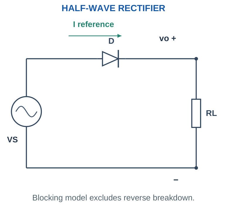
With a capacitor charged near +Vm, the source can later approach -Vm, giving a reverse stress near 2Vm in the ideal half-wave capacitor-input circuit. This is why the circuit condition must accompany a memorised PIV formula.
Trick
Write HWR + no C → Vm; HWR + reservoir C → approximately 2Vm under the ideal peak-hold model. Identify the capacitor before selecting the rule.
Worked problem 1.20: PIV with and without reservoir
Problem. A positive HWR has an ideal input peak of 15 V. Compare diode PIV with a resistive load alone and with an ideal peak-holding reservoir capacitor.
Model / approach. Use the stated ideal steady peak cases, excluding transients and forward drops.
Step 1. Without C, the blocked diode sees source peak: PIV = 15 V.
Step 2. With C holding about +15 V while input approaches -15 V, reverse stress is approximately 30 V.
Answer: 15 V unfiltered; about 30 V with peak-hold C.
Check and interpretation. The capacitor changes the reverse-stress circuit. A real part choice needs suitable rating margin and conditions; the exercise calculates ideal stress, not a final selected component.
Worked problem 1.21: Ripple ratio or percentage?
Problem. An ideal HWR uses a 50 Hz source. Find its ripple repetition frequency and RMS ripple factor.
Model / approach. Use the unfiltered sinusoidal HWR relations.
Step 1. One pulse occurs each source cycle, so fr = 50 Hz.
Step 2. r = √(π²/4 – 1) ≈ 1.2114; percentage ≈ 121.14%.
Answer: 50 Hz; r ≈ 1.2114 = 121.14%.
Check and interpretation. It is possible for RMS ripple to exceed the average output. Writing 1.21% would confuse the dimensionless value with its percentage representation.
17. FULL-WAVE BRIDGE: FOUR DIODES, TWO PATHS
A bridge uses four diodes arranged so that load current has the same direction for both input polarities. Label the AC nodes A and B, DC positive P and DC negative N. In this book’s bridge: D1 connects A→P, D2 B→P, D3 N→A and D4 N→B, where each arrow indicates its forward direction.
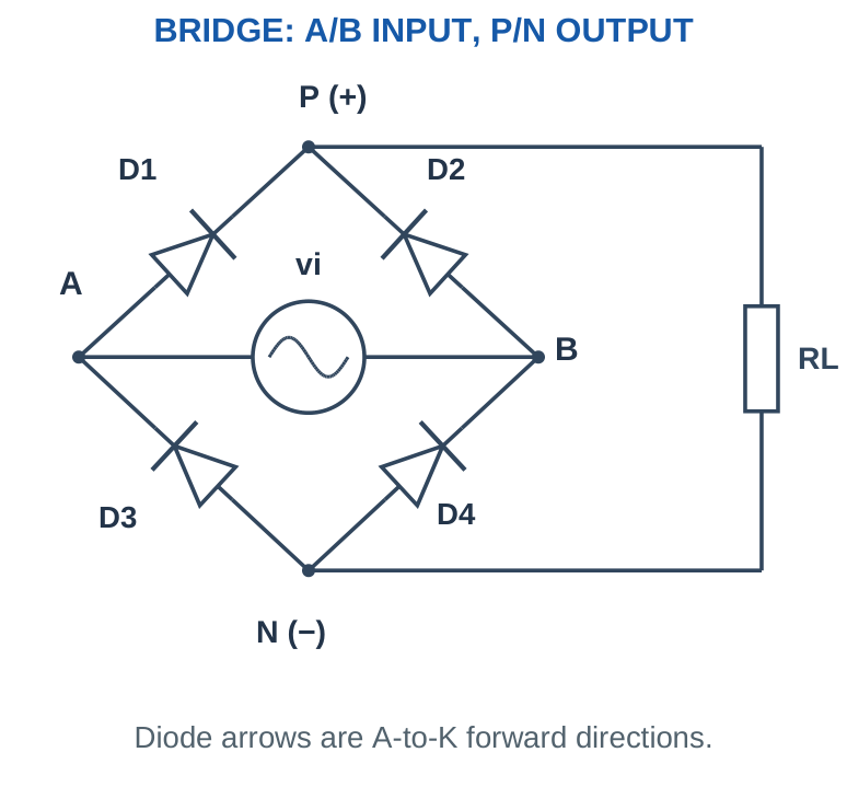
When A is positive relative to B, the path is A → D1 → P → RL → N → D4 → B. When B is positive, the path is B → D2 → P → RL → N → D3 → A. In both cases, current through RL goes from P to N. Two forward drops are in series with the load during conduction.
Bridge memory trick
The cathodes of the two upper-path diodes meet at DC positive. The anodes of the two lower-path diodes meet at DC negative. Trace actual A/K terminals instead of assuming the drawing’s top or bottom orientation is universal.
18. BRIDGE CONDUCTION: POSITIVE AND NEGATIVE

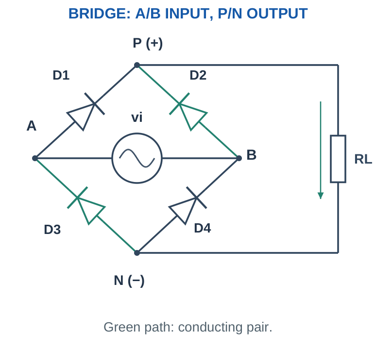
The word “negative half-cycle” refers to the chosen AC input reference, not a negative output across the load. Both halves are used to create same-polarity pulses. Each diode conducts during alternate half-cycles in the ideal symmetric resistive-load case. For a constant VF per conducting diode, the load voltage is vo = max(|vi| – 2VF, 0). Near each input zero crossing, the assumed source voltage may be too small to overcome both drops, so the real-model waveform does not exactly follow |vi| at all instants.
Exam method
Write a two-row conduction table with input polarity, conducting pair, blocked pair and load-current direction. This checks the diagram more effectively than memorising only “two diodes conduct.”
Worked problem 1.22: Instantaneous bridge state
Problem. For the labelled bridge, vi = vA – vB = 10 V. Each conducting diode uses VF = 0.7 V and RL = 1000 Ω. Find output and the conducting pair if current flows.
Model / approach. Use vo = max(|vi| – 2VF, 0); P is the positive load terminal.
Step 1. Available load voltage = max(10 – 2 × 0.7, 0) = 8.6 V.
Step 2. IL = vo/RL = 8.6 mA. The conducting pair is D1 and D4.
Answer: vo = 8.6 V; IL = 8.6 mA.
Check and interpretation. The output stays nonnegative for either input sign in this circuit. The input sign selects the pair; it does not reverse the intended P-to-N load current.
Worked problem 1.23: Instantaneous bridge state
Problem. For the labelled bridge, vi = vA – vB = -10 V. Each conducting diode uses VF = 0.7 V and RL = 1000 Ω. Find output and the conducting pair if current flows.
Model / approach. Use vo = max(|vi| – 2VF, 0); P is the positive load terminal.
Step 1. Available load voltage = max(10 – 2 × 0.7, 0) = 8.6 V.
Step 2. IL = vo/RL = 8.6 mA. The conducting pair is D2 and D3.
Answer: vo = 8.6 V; IL = 8.6 mA.
Check and interpretation. The output stays nonnegative for either input sign in this circuit. The input sign selects the pair; it does not reverse the intended P-to-N load current.
19. FULL-WAVE BRIDGE CALCULATIONS
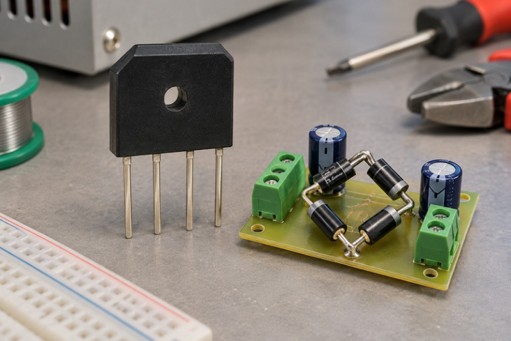
Component view 4. A packaged bridge rectifier and a bridge-supply assembly.
For a sinusoidal source, ideal bridge, no capacitor and resistive load: VDC = 2Vm/π; Vrms = Vm/√2; IDC = 2Im/π; Irms = Im/√2. The ideal full-wave output RMS equals the input sinusoidal RMS because changing sign does not change the squared waveform.
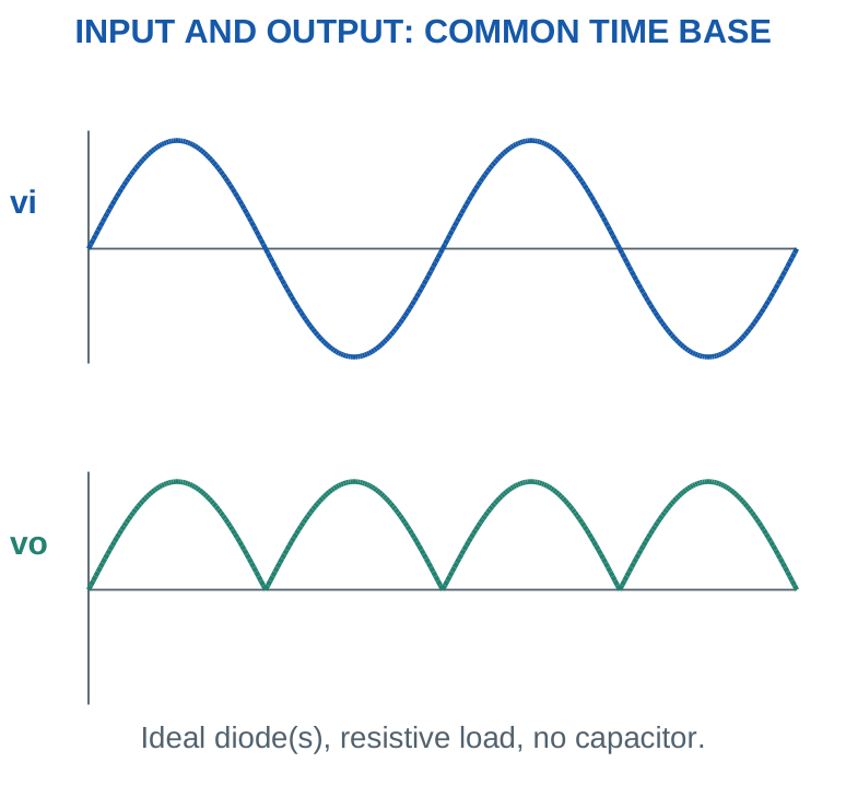
The ideal unfiltered full-wave ripple factor is √(π²/8 – 1) ≈ 0.483, commonly quoted as 0.482 with rounded constants. Conventional maximum rectification efficiency is 8/π² ≈ 81.1%, often quoted about 81.2%. Use consistent rounding rather than treating these close textbook values as fundamentally different circuits.
For nonzero drops, 2(Vm – 2VF)/π is a rough peak-scaled estimate, not an exact average of max(|vi| – 2VF, 0). The conduction-angle treatment later in this unit gives the more accurate result for that model. State which approximation you use.
Worked problem 1.24: Complete ideal bridge calculation
Problem. An ideal unfiltered bridge receives 12 V RMS sinusoidal input at 50 Hz and feeds 1000 Ω. Find input peak, output average/RMS, average load current and ripple frequency.
Model / approach. Ideal diodes; no capacitor; purely resistive load.
Step 1. Vm = √2 × 12 = 16.9706 V.
Step 2. VDC = 2Vm/π ≈ 10.8038 V; total output Vrms = 12 V.
Step 3. IDC = VDC/1000 ≈ 10.8038 mA; fr = 2 × 50 = 100 Hz.
Answer: VDC ≈ 10.8038 V; IDC ≈ 10.8038 mA.
Check and interpretation. The output RMS equals the input RMS in this ideal sign-reversal model. Its average is smaller than its RMS because it still contains a time-varying component.
Worked problem 1.25: Bridge diode average current
Problem. An ideal symmetric unfiltered bridge supplies average load current 100 mA. Find the average current in one diode over a full source cycle.
Model / approach. Each diode carries the load waveform during alternate half-cycles.
Step 1. A particular diode conducts for one of the two equal output pulses per source cycle.
Step 2. Its full-cycle average is IDC,load/2 = 100/2 = 50 mA.
Answer: Average per diode = 50 mA.
Check and interpretation. The instantaneous conducting diode current equals the instantaneous load current; it is not halved during conduction. This symmetry result must not be confused with peak charging current in a capacitor-input circuit.
20. RECTIFIER COMPARISON AND REVERSE STRESS
| Quantity: ideal, unfiltered, resistive load | Half wave | Bridge |
|---|---|---|
| Devices / conducting at a time | 1 / 1 | 4 / 2 |
| VDC in terms of input peak | Vm/π | 2Vm/π |
| Total Vrms | Vm/2 | Vm/√2 |
| Ripple repetition | f | 2f |
| Diode PIV | Vm | Vm per diode |
| Output pulses/source cycle | One | Two |
A centre-tapped full-wave rectifier is a different topology: it uses a centre-tapped secondary and two diodes, usually one conducting per half-cycle. Its diode reverse stress and the meaning of its quoted secondary voltage differ. This is a comparison note; the required full-wave topology in this syllabus is the bridge.
A bridge with a reservoir capacitor also needs its actual source and charging conditions considered. In the ordinary ideal bridge capacitor-input arrangement, diode reverse stress is of the order of the AC peak, unlike the approximately 2Vm half-wave capacitor case. Add margin and transient analysis when selecting real hardware; the ideal result is a circuit stress calculation, not a complete part qualification.
Worked problem 1.26: Same source, different average
Problem. A 10 V-peak sine feeds either an ideal HWR or an ideal bridge, each without C. Find both averages and their ratio.
Model / approach. Compare the same peak input and the same ideal resistive-load conditions.
Step 1. HWR: 10/π ≈ 3.1831 V.
Step 2. Bridge: 20/π ≈ 6.3662 V. Ratio = 2.
Answer: The bridge average is twice the HWR average in this model.
Check and interpretation. Real diode drops can reduce this exact ratio, especially for low source voltages. Adding a reservoir changes both waveforms, so this no-filter comparison should not be copied unchanged to filtered supplies.
21. NONZERO DROPS: CHOOSE THE RIGHT APPROXIMATION
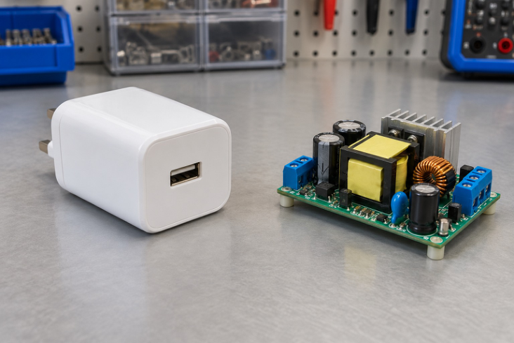
Component view 5. An illustrative USB charger and its internal switching-supply assembly.
For a constant-drop bridge, let a = 2VF and define α = sin-1(a/Vm) when Vm > a. Conduction in each rectified half-cycle occurs from α to π – α. The average of the clipped output is VDC = [2Vm cos α – a(π – 2α)]/π, with α in radians. This is optional worked enrichment; the basic peak and current calculations need no heavy semiconductor derivation.
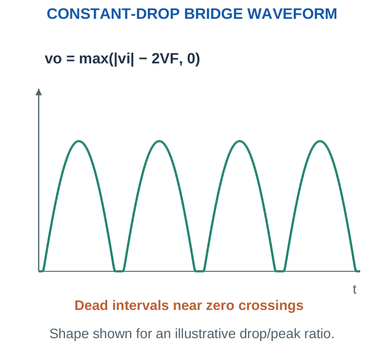
If Vm ≤ a, the assumed bridge model has no forward conduction. For half wave with a single constant drop a = VF, the corresponding average is [2Vm cos α – a(π – 2α)]/(2π). These relations describe the specified constant-drop, no-filter, resistive-load waveform, not a capacitor-input supply.
Calculation trick
For simple peak questions, subtract the conducting drops directly. For exact average questions, account for the zero-crossing dead interval or use the explicitly requested textbook approximation. Never label a convenient estimate “exact.”
Worked problem 1.27: Average including the dead interval
Problem. An unfiltered bridge has a 10 V peak sine and VF = 0.7 V for each conducting diode. Find the average using the constant-drop clipping model.
Model / approach. Output is max(|vi| – 2VF, 0), not a uniformly scaled sine.
Step 1. a = 2VF = 1.4 V; α = asin(a/Vm) = 0.1405 rad.
Step 2. VDC = [2Vm cos α – a(π – 2α)]/π ≈ 5.0287 V.
Step 3. The peak-scaled estimate 2(Vm – a)/π gives 5.4749 V; it is not the exact average.
Answer: Constant-drop-model average ≈ 5.0287 V.
Check and interpretation. The calculation uses radians in the average formula. It belongs to an unfiltered resistive-load bridge; a charged reservoir would change both conduction timing and the output average.
Worked problem 1.28: Average including the dead interval
Problem. An unfiltered bridge has a 1 V peak sine and VF = 0.7 V for each conducting diode. Find the average using the constant-drop clipping model.
Model / approach. Output is max(|vi| – 2VF, 0), not a uniformly scaled sine.
Step 1. Two-drop threshold a = 1.4 V exceeds source peak 1 V.
Step 2. The assumed constant-drop model therefore gives no conducting interval and VDC = 0.
Answer: VDC = 0 in the specified model.
Check and interpretation. The calculation uses radians in the average formula. It belongs to an unfiltered resistive-load bridge; a charged reservoir would change both conduction timing and the output average.
22. WHY A FILTER CAPACITOR WORKS
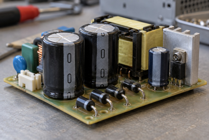
Component view 6. Reservoir capacitors reduce ripple; polarity and voltage rating remain important.
A reservoir capacitor connects in parallel with the load on the rectified side. It charges when the rectified source can exceed the capacitor voltage plus the conducting diode drops. Between those intervals, the capacitor supplies load current and its voltage falls. It stores energy; it does not generate additional charge or regulate the output by itself.
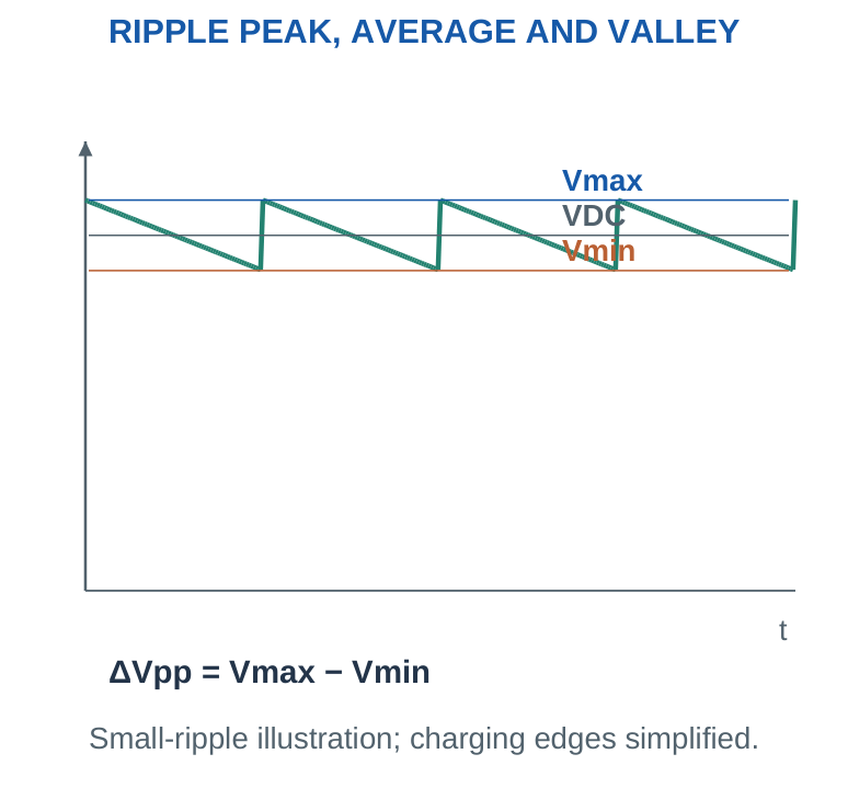
Increasing C generally reduces the droop for a given load and recharge rate under the small-ripple model. Increasing load current generally increases droop. A full-wave bridge recharges twice per source cycle, reducing the discharge interval compared with half wave at the same source frequency.
Connection trick
Filtering capacitor goes across the load in this reservoir circuit. Putting it in series creates a different circuit and does not reproduce the intended DC supply path.
23. RIPPLE ESTIMATION AND CAPACITOR SIZING
For approximately constant load current and small ripple, charge balance gives ΔQ ≈ IL Δt and ΔVpp ≈ ΔQ/C. With recharge frequency fr, take Δt ≈ 1/fr, giving ΔVpp ≈ IL/(fr C). Half wave uses fr = f; bridge full wave uses fr = 2f. Convert microfarads to farads and milliamperes to amperes before substituting. The average reservoir voltage can be estimated as VDC ≈ Vpk,out – ΔVpp/2 for a small, roughly sawtooth-like ripple. The minimum is approximately Vmin ≈ Vpk,out – ΔVpp. These are not identical quantities. A downstream regulator must have sufficient input even at the minimum of the ripple cycle.
Mental arithmetic
At 50 Hz mains frequency, bridge recharge is 100 Hz. With 100 mA load and 1,000 µF capacitance, ΔVpp ≈ 0.1/(100 × 0.001) = 1 V. Scale from this only while the same model and frequency apply.
The approximation ignores detailed charging angle, source impedance and capacitor ESR. If predicted ripple is comparable to the peak voltage, the small-ripple assumption is poor; do not interpret a negative computed minimum as a physically correct normal supply waveform.
Worked problem 1.29: Estimate peak-to-peak ripple
Problem. A bridge reservoir circuit has source frequency 50 Hz, approximately constant load 100 mA and C = 1000 µF. Estimate ΔVpp.
Model / approach. Use ΔVpp ≈ IL/(frC); assume small ripple and brief recharge intervals.
Step 1. IL = 0.1 A; C = 0.001 F; fr = 100 Hz.
Step 2. ΔVpp ≈ 0.1/(100 × 0.001) = 1 V.
Answer: Estimated ripple ≈ 1 V peak-to-peak.
Check and interpretation. Check this ripple against the expected DC level before trusting the small-ripple approximation. The formula estimates voltage droop, not the peak current through the rectifier during charging.
Worked problem 1.30: Estimate peak-to-peak ripple
Problem. A bridge reservoir circuit has source frequency 60 Hz, approximately constant load 60 mA and C = 1000 µF. Estimate ΔVpp.
Model / approach. Use ΔVpp ≈ IL/(frC); assume small ripple and brief recharge intervals.
Step 1. IL = 0.06 A; C = 0.001 F; fr = 120 Hz.
Step 2. ΔVpp ≈ 0.06/(120 × 0.001) = 0.5 V.
Answer: Estimated ripple ≈ 0.5 V peak-to-peak.
Check and interpretation. Check this ripple against the expected DC level before trusting the small-ripple approximation. The formula estimates voltage droop, not the peak current through the rectifier during charging.
Worked problem 1.31: Estimate peak-to-peak ripple
Problem. A bridge reservoir circuit has source frequency 50 Hz, approximately constant load 250 mA and C = 2200 µF. Estimate ΔVpp.
Model / approach. Use ΔVpp ≈ IL/(frC); assume small ripple and brief recharge intervals.
Step 1. IL = 0.25 A; C = 0.0022 F; fr = 100 Hz.
Step 2. ΔVpp ≈ 0.25/(100 × 0.0022) = 1.1364 V.
Answer: Estimated ripple ≈ 1.1364 V peak-to-peak.
Check and interpretation. Check this ripple against the expected DC level before trusting the small-ripple approximation. The formula estimates voltage droop, not the peak current through the rectifier during charging.
Worked problem 1.32: Size a bridge reservoir
Problem. A full-wave bridge at 60 Hz supplies approximately 200 mA. Size ideal C for no more than 1 V peak-to-peak ripple in the small-ripple model.
Model / approach. Rearrange C ≥ IL/(2f ΔVpp).
Step 1. IL = 0.2 A; fr = 120 Hz.
Step 2. Cmin = 0.2/(120 × 1) = 0.0017 F = 1666.6667 µF.
Answer: Ideal minimum C ≈ 1666.6667 µF.
Check and interpretation. This is the required actual capacitance under the model. A nominal selected part must still account for tolerance, voltage stress and its operating conditions; rounding the nominal value down can violate the ripple target.
24. RESISTIVE LOAD AND APPROXIMATION CHECKS
When the load is a resistor rather than a specified constant-current load, IL depends on the output voltage: IL ≈ VDC/RL. Substituting into the small-ripple equations gives VDC ≈ Vpk,out/[1 + 1/(2fr CRL)]. Then calculate IL = VDC/RL and ΔVpp = IL/(fr C). This keeps the approximate load current consistent with the approximate average voltage.
An exact resistor-only discharge interval with no source conduction follows V(t) = V0 e-t/(RLC). Real rectifier charging resumes when the source overtakes the capacitor-plus-diode threshold; treating the entire period as a pure discharge is only a stated simplified interval calculation. A useful validity check is ΔVpp/VDC. A small ratio supports the simple small-ripple model; a large ratio suggests using a more detailed waveform or simulation. The definition of “small enough” depends on the desired accuracy rather than one universal boundary.
Exam habit
Write “approximately” in ripple answers. The charge-balance estimate is powerful because it is simple, not because every real supply waveform is exactly triangular.
Worked problem 1.33: Solve the resistive load consistently
Problem. The rectified charging peak is 8 V. A bridge at 60 Hz feeds RL = 800 Ω with C = 1000 µF. Estimate VDC, IL and ripple.
Model / approach. Use IL ≈ VDC/RL with the small-ripple reservoir equations.
Step 1. VDC ≈ 8/[1 + 1/(2 × 120 × 0.001 × 800)] = 7.9585 V.
Step 2. IL ≈ VDC/RL = 9.9482 mA.
Step 3. ΔVpp ≈ IL/(frC) = 0.0829 V; Vmin ≈ 7.9171 V.
Answer: VDC ≈ 7.9585 V; ΔVpp ≈ 0.0829 V.
Check and interpretation. Using the unrounded values, VDC + ΔVpp/2 equals the supplied charging peak. This is a self-consistent approximation, not an exact rectifier transient solution.
25. CAPACITOR CHARGE, ENERGY AND RATINGS
Capacitor charge is Q = CV and stored energy is E = ½CV². Doubling voltage doubles charge but quadruples stored energy at the same capacitance. These are different physical quantities. The peak capacitor voltage, including the highest intended input condition, matters for selecting a voltage rating. A capacitance tolerance affects ripple: minimum actual C gives the larger ripple for the same load and frequency. Equivalent series resistance, ESR, produces an additional voltage change when current changes. Capacitor ripple-current rating and thermal conditions also matter; capacitance and voltage rating alone do not describe every limit.
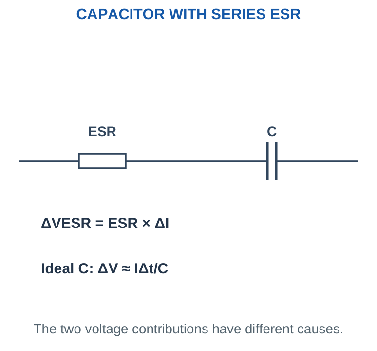
The initial uncharged reservoir can demand a charging pulse limited by source, wiring and device impedances. Therefore average load current is not the diode’s peak current. This unit calculates simple charge and energy quantities without pretending they determine a complete inrush waveform.
Rating trick
Use maximum expected reservoir voltage for voltage stress, minimum actual capacitance for the worst ripple estimate, and the stated thermal conditions for permitted operation. Do not use the average output voltage as the capacitor’s maximum stress.
Worked problem 1.34: Capacitance tolerance
Problem. A 1,000 µF reservoir has a -20% minimum tolerance. A bridge recharges at 100 Hz and supplies 80 mA. Find the worst ripple due to this capacitance tolerance alone.
Model / approach. Use minimum actual C for maximum charge-balance ripple.
Step 1. Cmin = 1,000 × 0.80 = 800 µF = 0.0008 F.
Step 2. ΔVpp ≈ 0.080/(100 × 0.0008) = 1 V.
Answer: Worst estimated ripple from C tolerance = 1 Vpp.
Check and interpretation. Nominal capacitance would predict 0.8 Vpp. The tolerance changes the estimate by 25% relative to that nominal result; a 20% capacitance reduction does not cause only a 20% ripple increase because ripple is inversely proportional to C.
26. RIPPLE FACTOR AFTER FILTERING
Ripple peak-to-peak ΔVpp and ripple RMS Vr,ac,rms are different. For a zero-mean triangular or sawtooth ripple approximation, Vr,ac,rms ≈ ΔVpp/(2√3). Ripple factor is then r ≈ ΔVpp/(2√3 VDC). The percentage is 100r.
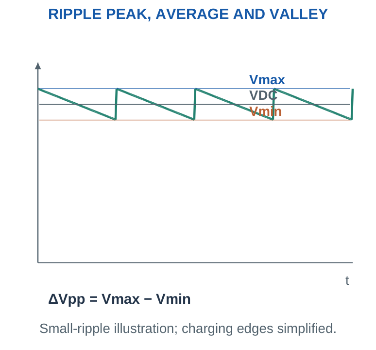
The ideal unfiltered factors near 1.21 and 0.483 must not be reused after a reservoir capacitor changes the waveform. Similarly, the small triangular-ripple RMS expression must not be applied to an arbitrary pulse waveform without checking its shape. Given measured total output RMS and average, Vr,ac,rms = √(Vrms,total² – VDC²), provided the measurement definitions and bandwidth are appropriate. A meter’s AC range may or may not measure the same quantity assumed in a textbook calculation; know the instrument mode before interpreting a reading.
Percentage trick
r = 0.02 means 2%, not 0.02%. ΔVpp/VDC is a peak-to-peak ripple ratio, not the RMS ripple factor defined above.
Worked problem 1.35: Convert ripple measures
Problem. A filtered output has VDC = 12 V and approximately triangular ripple of 1 V peak-to-peak. Find ripple RMS and ripple factor.
Model / approach. Use zero-mean triangular-ripple approximation.
Step 1. Vr,ac,rms ≈ 1/(2√3) = 0.2887 V.
Step 2. r = Vr,ac,rms/VDC ≈ 0.0241; percentage ≈ 2.4056%.
Answer: Ripple RMS ≈ 0.2887 V; r ≈ 2.4056%.
Check and interpretation. The peak-to-peak ripple ratio is a different quantity. For a different ripple shape, the RMS conversion factor can change; the stated triangular approximation is part of this answer.
27. ZENER DIODE AND REVERSE BREAKDOWN
A Zener diode is used in a specified reverse-breakdown region where a substantial current change can occur with a relatively small voltage change. Its cathode is connected toward the positive rail in the usual positive shunt-regulator circuit. In forward bias it behaves broadly like a normal silicon junction.
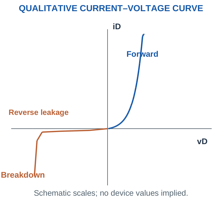
The physical mechanisms include Zener tunnelling and avalanche multiplication. Their relative importance depends on junction properties and breakdown voltage; practical parts called “Zener diodes” can involve either or both. Avoid claiming all breakdown is destructive or that all breakdown mechanisms are identical. A nominal VZ is specified at a test current and temperature with a tolerance. Dynamic resistance, knee behaviour and temperature dependence affect the actual operating voltage. For initial circuit problems, a constant VZ model is used explicitly; later problems add a supplied dynamic resistance or tolerance.
Orientation trick
For a positive Zener regulator, the cathode faces the positive output, the anode faces the return, and a series resistor limits current from the source. Reversing it generally gives ordinary forward conduction rather than the desired reverse reference.
28. ZENER SHUNT REGULATOR: CURRENT SPLITTING
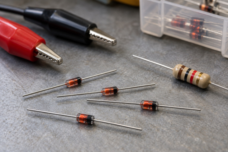
Component view 7. Zener diodes with a test instrument: device identity and the stated test conditions matter.
A series resistor RS feeds an output node. The reverse-biased Zener and load RL connect in parallel from that node to return. In the constant-VZ regulating state, IS = (VS – VZ)/RS, IL = VZ/RL, and IZ = IS – IL. Apply KCL at the output node.
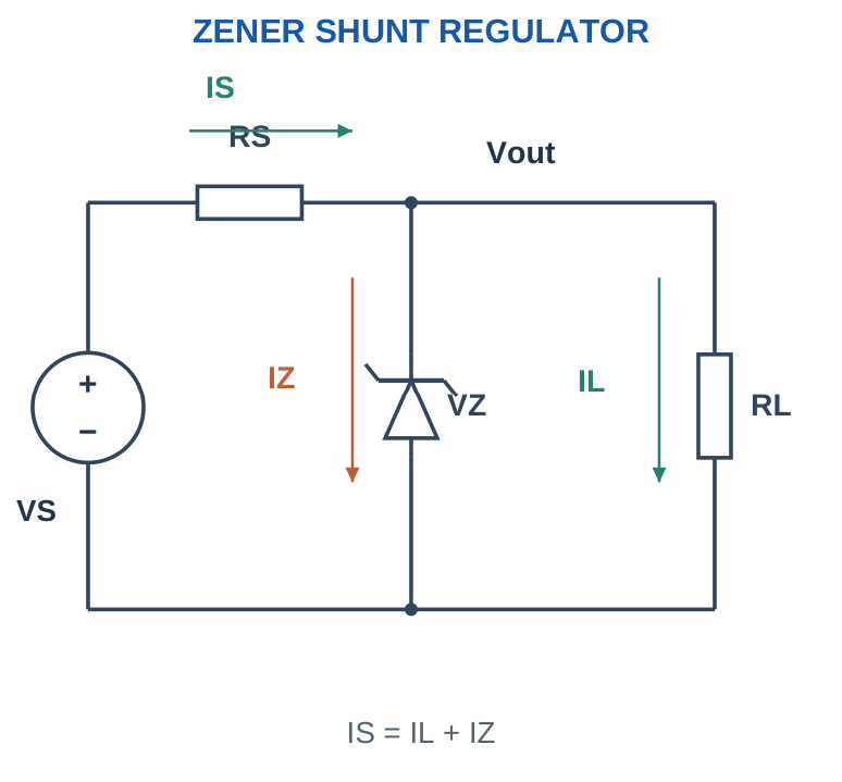
Regulation requires the Zener to remain within its useful current range and power limit. If the calculation gives IZ below a specified IZ,min, the assumed regulation condition is not met. If it gives negative IZ, the constant-VZ conducting assumption is impossible for the illustrated reverse Zener branch.
Current trick
Draw one arrow into the node and two arrows out. Source current does not automatically equal Zener current after connecting a load. No-load is a special case where IL = 0 and all series current flows through the Zener.
Worked problem 1.36: Find all three currents
Problem. A Zener shunt stage has VS = 12 V, VZ = 5.1 V, RS = 330 Ω and RL = 1000 Ω. Assume constant-VZ regulation and find IS, IL, IZ and Zener dissipation.
Model / approach. Test the regulating state using KCL at the output.
Step 1. IS = (12 – 5.1)/330 = 20.9091 mA.
Step 2. IL = 5.1/1000 = 5.1 mA; IZ = IS – IL = 15.8091 mA.
Step 3. PZ = VZ IZ ≈ 0.0806 W.
Answer: IZ ≈ 15.8091 mA; PZ ≈ 80.6264 mW.
Check and interpretation. The calculated IZ is positive. If a minimum regulating current or allowed power is supplied, compare those limits before accepting the regulation assumption. Source current is shared; it is not all Zener current.
29. REGULATION CHECK AND THE OFF-STATE DIVIDER
Always test the regulating assumption before reporting Vout = VZ. If the reverse Zener is OFF in the simple resistor circuit, the source, RS and RL form a voltage divider: Vout = VS RL/(RS + RL). Compare that result with the breakdown requirement under the stated model.
A computed IZ that is positive but smaller than a specified minimum current may mean the part is near or below its intended regulation region. A sharp ideal-Zener model and a real minimum-current specification describe different levels of approximation. State the criterion used.
Trap question
A 5.1 V Zener connected to a 5 V source through a resistor cannot produce a regulated 5.1 V output in this passive circuit. A Zener shunt stage is not a voltage-boost converter.
Worked problem 1.37: Reject an impossible regulating state
Problem. VS = 5 V, VZ = 5.1 V, RS = 330 Ω, RL = 1000 Ω. Use an ideal reverse Zener model and determine the actual output state.
Model / approach. Assume Vout = VZ, calculate IZ, then solve the OFF divider if the assumption fails.
Step 1. Assumed IZ = (5 – 5.1)/330 – 5.1/1000 = -5.403 mA, which is negative.
Step 2. Zener OFF: Vout = 5 × 1000/(330 + 1000) = 3.7594 V.
Answer: Zener OFF; Vout ≈ 3.7594 V.
Check and interpretation. The divider output is below VZ, so the OFF state is self-consistent in this model. Reporting the nominal Zener voltage after obtaining negative IZ would contradict the assumed circuit direction.
30. INPUT AND LOAD REGULATION WINDOWS
For a given RS, a regulating Zener must retain enough current at the lowest input and highest load. It must not exceed its allowed current or power at the highest input and lowest load. These are different corner cases.
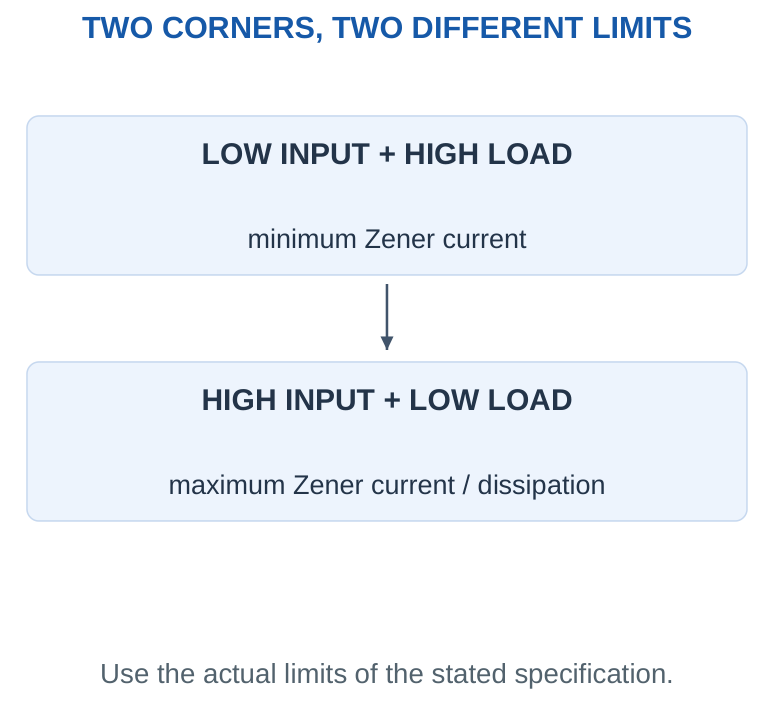
For a specified load current, VS,min = VZ + RS(IL + IZ,min). For a stated maximum useful Zener current, VS,max = VZ + RS(IL + IZ,max). At fixed VS, the largest allowed load current is IL,max = (VS – VZ)/RS – IZ,min, if that result is nonnegative and other conditions are satisfied. A resistive load has IL ≈ VZ/RL while regulation holds. As RL decreases, load current increases and Zener current decreases. As RL increases toward no-load, Zener current increases. This is a useful direction check before substituting numbers.
Corner memory trick
Weak source + hungry load → Zener starved. Strong source + light load → Zener hottest. Use this to choose the correct extremes before doing algebra.
Worked problem 1.38: Maximum load current
Problem. VS = 12 V, VZ = 5.1 V, RS = 330 Ω and required IZ,min = 5 mA. Find maximum load current and corresponding minimum resistive load.
Model / approach. At the current-limit boundary, retain exactly IZ,min in the Zener.
Step 1. IL,max = (12 – 5.1)/330 – 0.005 = 15.9091 mA.
Step 2. RL,min = VZ/IL,max ≈ 320.5714 Ω.
Answer: IL,max ≈ 15.9091 mA; RL,min ≈ 320.5714 Ω.
Check and interpretation. A smaller load resistance demands more current and can starve the Zener. A larger resistance is not the worst starvation case, although it can increase Zener dissipation by reducing load current.
Worked problem 1.39: Minimum input voltage
Problem. A 5.1 V Zener stage uses RS = 330 Ω, fixed load current 10 mA and IZ,min = 5 mA. Find the minimum source voltage for the stated regulating-current requirement.
Model / approach. Apply VS,min = VZ + RS(IL + IZ,min).
Step 1. Required series current = 0.010 + 0.005 = 0.015 A.
Step 2. VS,min = 5.1 + 330 × 0.015 = 10.05 V.
Answer: Minimum source = 10.05 V in this model.
Check and interpretation. This is the low-input boundary. The high-input/no-load power condition remains a separate check and is not established by calculating the minimum voltage alone.
31. SELECTING RS AND CHECKING POWER
The low-current requirement gives RS ≤ (VS,min – VZ)/(IL,max + IZ,min). The high-current requirement gives RS ≥ (VS,max – VZ)/(IL,min + IZ,max). A valid simple solution exists only when the lower bound does not exceed the upper bound, using positive quantities and compatible assumptions. If the Zener’s permitted dissipation is PZ,allow, a simple constant-voltage current limit is IZ,max = PZ,allow/VZ. A real selection also follows thermal derating and operating conditions. Resistor dissipation is (VS – VZ)²/RS while regulation holds, so its high-input case must be checked.
No available RS interval means the specifications cannot all be met by this simple constant-Zener arrangement. Do not pick an arbitrary midpoint outside the interval. Adjust the requirements or use another suitable regulation approach.
Design trick
Solve the inequalities first; select a standard resistor second; verify the actual selected value third. A theoretical resistance value is not a finished design decision.
Worked problem 1.40: Design and verify a resistor interval
Problem. Input = 8–12 V; VZ = 3.3 V; load = 0–12 mA; IZ,min = 4 mA. Allowed Zener dissipation is 0.25 W. Check a selected RS = 270 Ω.
Model / approach. Use the supplied allowed power and constant-VZ model; resistor tolerance is neglected in this exercise.
Step 1. IZ,max = 0.25/3.3 = 75.7576 mA.
Step 2. RS,min = (12 – 3.3)/(0 + 0.0758) = 114.84 Ω.
Step 3. RS,max = (8 – 3.3)/(0.012 + 0.004) = 293.75 Ω. 270 Ω lies inside.
Step 4. Low corner IZ = 5.4074 mA. High corner IZ = 32.2222 mA; PZ = 0.1063 W; PR = 0.2803 W.
Answer: 270 Ω satisfies the stated current/power window.
Check and interpretation. The selected value is rechecked rather than assumed valid from rounding. Resistor power capability and real thermal/tolerance conditions are additional component-selection inputs beyond this simplified allowed-power calculation.
Worked problem 1.41: When no resistor can satisfy the specification
Problem. Input is 8–16 V, VZ = 5 V, load is 0–20 mA, IZ,min = 5 mA and IZ,max = 30 mA. Determine whether any RS meets both current corners.
Model / approach. Solve the lower and upper bounds before selecting a resistance.
Step 1. RS ≥ (16 – 5)/(0 + 0.030) = 366.6667 Ω.
Step 2. RS ≤ (8 – 5)/(0.020 + 0.005) = 120 Ω.
Answer: There is no overlapping RS interval.
Check and interpretation. A midpoint cannot fix incompatible bounds. The simple shunt arrangement cannot meet all these assumptions simultaneously; the requirements or regulation approach must change. This is a valid design conclusion, not an arithmetic failure.
Worked problem 1.42: Check resistor tolerance after selection
Problem. For VS = 12 V and VZ = 5.1 V, RS = 330 Ω ±5%, and fixed IL = 10 mA, find the Zener-current range.
Model / approach. Use Rmax for minimum series current and Rmin for maximum series current.
Step 1. Rmin = 313.5 Ω; Rmax = 346.5 Ω.
Step 2. IZ,min = 6.9/346.5 – 0.010 ≈ 9.9134 mA.
Step 3. IZ,max = 6.9/313.5 – 0.010 ≈ 12.0096 mA.
Answer: Zener current ≈ 9.9134–12.0096 mA.
Check and interpretation. Any required minimum-current and power constraints must be checked against these extremes. Choosing a nominal resistance inside a nominal interval does not automatically cover its tolerance.
32. ZENER TOLERANCE, DYNAMIC RESISTANCE AND EFFICIENCY
With a supplied small-signal dynamic resistance rz, a local current change produces approximately ΔVZ = rz ΔIZ around the specified operating point. This is a local approximation, not a rule to extend through zero current and across the whole characteristic. A tolerance such as ±5% describes a permitted voltage interval under stated test conditions. It does not mean the Zener can carry any current within that same percentage. Temperature coefficients also require their stated units and reference conditions.
For the simple shunt stage, useful-load efficiency is approximately (VZ IL)/(VS IS). At no load the useful-load power is zero even though resistor and Zener dissipation can remain significant. This helps explain why a small reference circuit should not be presented as a universal high-current supply for a computer board.
Interpretation trick
Voltage accuracy, load capability and efficiency are separate. Getting 3.3 V in one no-load calculation does not establish a usable regulated supply over a real board’s changing current demand.
Worked problem 1.43: Dynamic-resistance correction
Problem. A Zener is 5.10 V at 10 mA and has supplied local rz = 8 Ω. Estimate its voltage at 15 mA using the linearised model.
Model / approach. Use ΔVZ = rz ΔIZ around the given point.
Step 1. ΔIZ = 15 – 10 = 5 mA = 0.005 A.
Step 2. ΔVZ = 8 × 0.005 = 0.040 V; new voltage ≈ 5.14 V.
Answer: Estimated local voltage = 5.14 V.
Check and interpretation. This is a small-range model. Do not extend it through zero current or use 5.10 V / 10 mA as the dynamic resistance; that point ratio would be a different quantity.
33. LED WORKING AND POLARITY
An LED is a semiconductor diode that emits light through radiative carrier recombination under suitable forward operation. Its material system influences emitted wavelength. Forward voltage depends on the device, current and temperature; a colour is not a guarantee of one exact drop for every component.
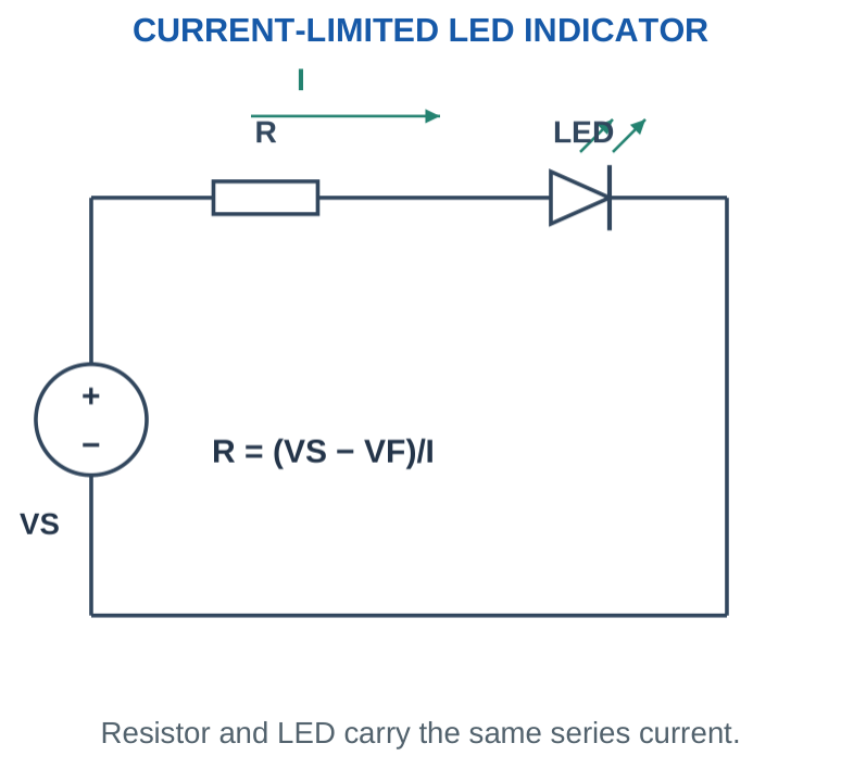
The useful design variable for a basic indicator is its permitted forward current. Directly connecting an LED to an ideal voltage source without a current-limiting mechanism is not the intended circuit. A resistor is a simple low-current method; more demanding applications can use regulated-current drivers. The longer-lead/flat-edge identification conventions of many through-hole LEDs can help, but cut leads, packages and internal structures vary. Use the specific component’s documentation. An LED’s reverse rating is also distinct from its forward operating voltage.
Memory trick
LED arrows point out because light comes out. This drawing cue does not replace the A/K orientation needed for current calculation.
34. LED CURRENT-LIMITING RESISTOR
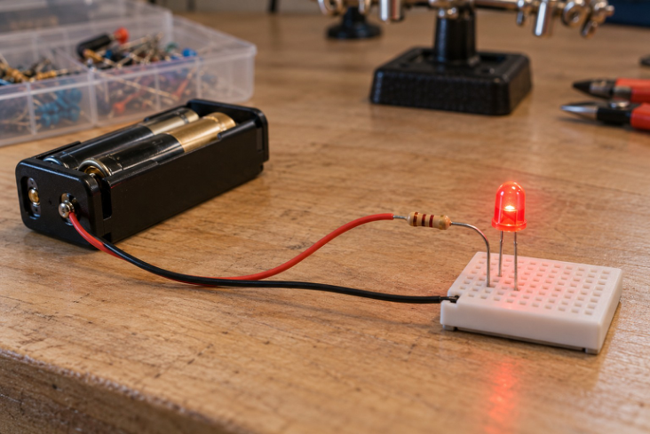
Component view 8. An LED indicator with a series resistor in a low-voltage circuit.
For a source VS, one LED of assumed forward drop VF and target current I, R = (VS – VF)/I. The resistor drops VS – VF, not the entire source voltage. If the source does not provide the required forward voltage and headroom, the assumed operating point cannot be obtained with a passive resistor.
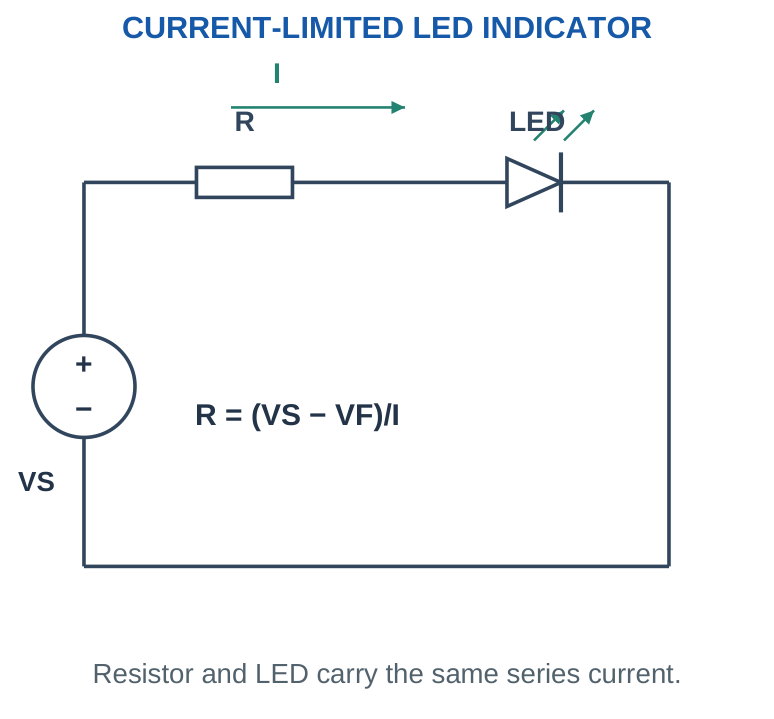
After choosing a resistor, recalculate I = (VS – VF)/Ractual. Resistor power is (VS – VF)I. For a current ceiling under the constant-drop model, selecting the next higher available resistance can reduce current relative to the target, but tolerance and supply/device extremes must still be considered.
Unit trick
Using volts divided by milliamperes gives kilohms. Example: 3 V / 10 mA = 0.3 kΩ = 300 Ω. Write the unit explicitly so that 10 mA is not accidentally treated as 10 A.
Worked problem 1.44: Calculate, select and recalculate
Problem. An LED uses assumed VF = 2 V from a 5 V source. Target is 10 mA. Find ideal R, then evaluate an available 330 Ω resistor.
Model / approach. Series resistor limits current in the constant-forward-drop model.
Step 1. Rideal = (5 – 2)/0.01 = 300 Ω.
Step 2. With 330 Ω, I = (5 – 2)/330 = 9.0909 mA.
Step 3. PR = I²R ≈ 27.2727 mW.
Answer: Ideal R = 300 Ω; selected current ≈ 9.0909 mA.
Check and interpretation. The selected resistor changes the current, so report the recalculated value. This nominal exercise does not include source, resistor or LED tolerance; those are checked in the following cases.
35. LED TOLERANCE AND POWER CHECKS
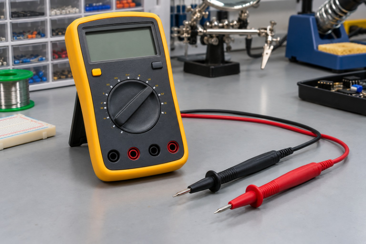
Component view 9. A multimeter supports polarity, voltage and continuity checks under the correct setup.
For a resistor-limited LED, the highest current uses VS,max, VF,min and Rmin. With resistor tolerance t, Rmin = Rnom(1 – t). The lowest current uses VS,min, VF,max and Rmax. Use compatible assumed ranges for the same operating scenario.
A practical current ceiling calculation can require Rnom ≥ (VS,max – VF,min)/[Imax(1 – t)]. After selecting a nominal value, check actual current and resistor dissipation over the stated range. A nominal 10 mA calculation alone does not guarantee a 10 mA maximum. The LED dissipates approximately VF I electrically at the terminals, but not all of that becomes emitted optical power. Do not calculate luminous brightness or efficiency from forward voltage and current alone unless the needed optical data are supplied.
Check before rounding
Round a current-limiting resistance in the direction consistent with the design requirement. “Nearest” is not always appropriate when the problem specifies an absolute maximum current.
Worked problem 1.45: Worst current corners
Problem. VS = 4.75–5.25 V, VF = 1.8–2.2 V and R = 330 Ω ±5%. Find current extremes under this model.
Model / approach. Maximum current combines VS,max, VF,min and Rmin; minimum current uses the opposite corner.
Step 1. Rmin = 313.5 Ω; Rmax = 346.5 Ω.
Step 2. Imax = (5.25 – 1.8)/313.5 ≈ 11.0048 mA.
Step 3. Imin = (4.75 – 2.2)/346.5 ≈ 7.3593 mA.
Step 4. At the high-current corner, resistor dissipation ≈ 37.9665 mW.
Answer: Current range ≈ 7.3593–11.0048 mA.
Check and interpretation. The assumed VF interval represents supplied problem limits. A real component’s operating curves and temperature conditions are needed to refine this conservative resistor-model check.
Worked problem 1.46: Design for a current ceiling
Problem. VS,max = 5.25 V, VF,min = 1.8 V, resistor tolerance ±5%, and permitted current ceiling 10 mA. Find minimum nominal R and check a 390 Ω selection.
Model / approach. Use minimum actual resistance at the high-current corner.
Step 1. Rnom ≥ (5.25 – 1.8)/[0.010 × 0.95] ≈ 363.1579 Ω.
Step 2. For 390 Ω nominal, Rmin = 370.5 Ω. Imax = 3.45/370.5 ≈ 9.3117 mA.
Answer: A 390 Ω selection meets this stated current ceiling.
Check and interpretation. An ideal nominal calculation of 345 Ω ignores resistor tolerance. Recheck the actual selected value at the specified extremes rather than assuming any nearby standard value is sufficient.
36. SERIES STRINGS AND PARALLEL BRANCHES
For n series LEDs, the same current passes through every LED and their assumed drops add: R = (VS – ΣVF)/I. Enough source voltage must remain for the resistor at the intended operating point. The number of LEDs is limited by the source and the required headroom, not only by physical space.
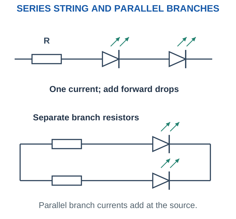
For parallel indicators, individual branch resistors let each branch establish its own approximate current. One shared resistor limits only total current and does not guarantee equal sharing between LEDs with different characteristics. Equal-looking devices can still have different forward drops.
Wiring trick
Series → add LED drops, keep one branch current. Parallel branches → same supply voltage, add branch currents. Do not multiply the desired current by the number of series LEDs when finding the one series resistor.
Worked problem 1.47: Series LED string
Problem. A 12 V source drives a string of 3 LEDs with assumed drops 2 V, 2 V, 2 V at 10 mA. Find the ideal one-branch resistor.
Model / approach. All series LEDs carry the same branch current.
Step 1. Sum of LED drops = 6 V; resistor drop = 6 V.
Step 2. R = (12 – 6)/0.01 = 600 Ω.
Answer: Ideal resistor = 600 Ω.
Check and interpretation. Do not multiply the target branch current by the number of series LEDs. Current is common in series; voltage drops add. Recalculate current after choosing a practical nominal value and checking tolerances.
Worked problem 1.48: Separate parallel indicators
Problem. Three parallel branches each contain a 2 V LED and a 300 Ω resistor across 5 V. Find nominal current in each branch and total source current.
Model / approach. Each branch has its own current-limiting resistor; use the constant-drop model.
Step 1. Branch current = (5 – 2)/300 = 10 mA.
Step 2. Total = 3 × 10 = 30 mA. Each resistor dissipates 3 × 0.010 = 30 mW.
Answer: 10 mA per branch; 30 mA total.
Check and interpretation. The identical supplied values give identical calculated currents, but real forward drops and tolerances can cause differences. One shared resistor would constrain only total current and would not establish the same independent branch behaviour.
37. 5 V AND 3.3 V SUPPLIES FOR ELECTRONIC BOARDS
A rail value is a voltage specification, not a complete supply specification. A board also needs adequate current, allowable ripple, transient response and the correct input connection. Board power inputs and GPIO signal pins have different functions.

Classic Arduino UNO R3 is a useful 5 V board example; other Arduino families can use different logic and supply arrangements. Raspberry Pi single-board computers commonly accept a 5 V-class input and provide 3.3 V GPIO signals, while specific models have their own input requirements. Do not apply 5 V directly to a 3.3 V GPIO because the board also has a 5 V power pin.
A resistor divider is not generally a regulated power supply: its output changes with load. A low-power Zener reference illustrates regulation but is not automatically appropriate for the current demand of a complete Raspberry Pi. Use board documentation for the actual product; the numerical exercises here use stated illustrative loads.
Application trick
Separate “what voltage?”, “how much current?”, “what ripple?” and “which terminal?”. Matching only the printed voltage number does not answer the full application question.
38. FILTER MINIMUM AND REGULATOR HEADROOM
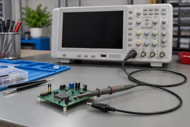
Component view 10. An oscilloscope reveals the waveform and peak-to-peak ripple at the measured node.
A regulator can maintain its intended output only while its input and load remain inside its specified operating range. For an illustrative linear regulator with a supplied required headroom H, the reservoir minimum should satisfy Vmin ≥ Vout + H. Use the ripple valley, not just the average or peak.
For a bridge-capacitor estimate, combine Vpk,out ≈ √2 Vs,rms – 2VF with ΔVpp ≈ IL/(2fC), then Vmin ≈ Vpk,out – ΔVpp. A problem may also require minimum source RMS, maximum load and minimum actual capacitance. Use those specified extremes together for the valley check. Linear-regulator dissipation can be estimated as (Vin – Vout)IL when quiescent current is neglected. More voltage headroom can improve a dropout margin while increasing heat. LDO and switching-converter internals belong mainly to later units; here the focus is reading the supply chain correctly.
Trick
“Peak is high enough” is not the same as “input is always high enough.” For a reservoir-fed regulator, check the bottom of the ripple first.
Worked problem 1.49: Check the ripple valley
Problem. A 50 Hz bridge uses 9 V RMS, VF = 0.7 V each, C = 1000 µF and approximate constant load 100 mA. A 5 V regulator requires supplied headroom 2 V. Check the estimated valley.
Model / approach. Use the small-ripple bridge estimate and supplied regulator threshold.
Step 1. Vpk,out ≈ √2 × 9 – 2 × 0.7 = 11.3279 V.
Step 2. ΔVpp ≈ 0.1/(100 × 0.001) = 1 V.
Step 3. Vmin ≈ 10.3279 V; required minimum = 5 + 2 = 7 V.
Answer: The estimated valley passes the stated headroom test.
Check and interpretation. This calculation checks only the stated voltage model. Input tolerance, capacitance tolerance, load changes and the regulator operating specification would also be needed for a complete real-board supply design.
39. USB CHARGER RECTIFIER: WHERE THE DIODE FITS
The rectifier is one functional stage in a charger. An AC-input switch-mode USB adapter can include an input bridge and reservoir, a controlled high-frequency conversion stage, an isolation transformer where required by the topology, secondary rectification and output regulation. Modern designs may use synchronous rectification rather than an ordinary diode in some stages.
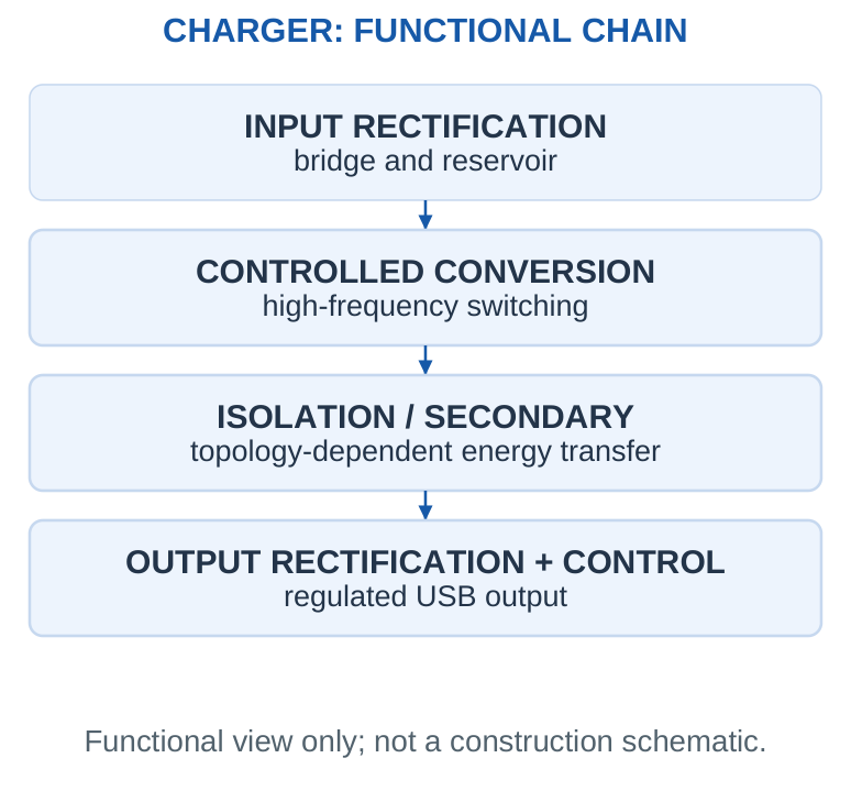
A bridge and capacitor alone do not turn an AC mains input into a regulated, isolated USB output. A transformer-based low-voltage classroom rectifier and a commercial switch-mode charger are related through rectification principles, but their complete topologies differ. The numerical circuit work in this unit uses specified low-voltage sources. A charger output label such as 5 V, 2 A describes an output capability under the relevant conditions. The actual load current depends on the connected device and its control, rather than the supply forcing the full labelled current through every load. USB negotiation details are outside Unit I.
Product-answer trick
Name rectification, energy conversion, isolation and regulation separately. Do not draw only four diodes and label the whole diagram “complete USB charger.”
Worked problem 1.50: Charger output versus source input
Problem. An illustrative charger delivers 5 V at 2 A and operates at 80% conversion efficiency at that point. Find output power, input power and loss.
Model / approach. Use efficiency = output power/input power at the same operating point.
Step 1. Pout = 5 × 2 = 10 W.
Step 2. Pin = 10/0.80 = 12.5 W. Loss = 12.5 – 10 = 2.5 W.
Answer: 10 W out, 12.5 W in, 2.5 W loss.
Check and interpretation. The input RMS current cannot be found accurately from these values alone without input voltage and power-factor information. A DC-side current rating should not be treated as the AC-input current.
40. TROUBLESHOOTING BY CIRCUIT FUNCTION
Start with the observed quantity and the expected stage behaviour. A half-wave waveform where a bridge output is expected can suggest a missing conduction path, but a waveform alone does not identify one unique failed component without additional checks. Low reservoir voltage can arise from load, source, capacitance, diode path or connection issues.
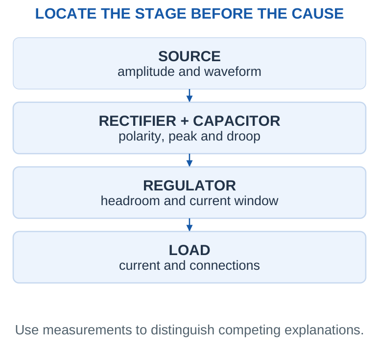
| Symptom in a stated simple circuit | Useful reasoning |
|---|---|
| LED dark | Check orientation, available voltage, branch current and continuity |
| Zener output below nominal | Test the regulating assumption and load current |
| Large droop | Compare IL, recharge frequency and actual C |
| Repeated regulator dropout | Compare the ripple minimum with required headroom |
| High resistor heating | Recalculate current and dissipation under actual conditions |
Exam habit
Give the condition, relevant equation and evidence needed. Avoid declaring one component faulty from a generic symptom that has several possible causes.
41. [B & C] PHOTODIODE; [C] PHOTOTRANSISTOR
Light detection. A photodiode is a light-sensitive semiconductor junction. Absorbed photons with sufficient energy create electron-hole pairs. Collection of these carriers produces a light-dependent current. An LED emits light; a photodiode detects incident light.
Reverse-biased operation. In photoconductive mode, the cathode is positive relative to the anode. Illumination increases the magnitude of the reverse photocurrent. Ordinary light detection does not require breakdown. Stay within the device reverse-voltage rating. Dark current is the current present without the intended illumination.
Zero-bias operation. A photodiode can also operate in photovoltaic mode without an externally applied reverse voltage. Its connected circuit determines the observed voltage and current. Reverse bias is therefore useful in some detector circuits, not essential in every application.
Readout. A suitable resistor or current-to-voltage amplifier converts the small photocurrent into a measurable voltage. In the simple resistive model, the magnitude of the light-dependent voltage change is approximately ΔV = ΔIphoto R while the circuit remains within its operating range. Higher R gives a larger change but can reduce speed or exhaust voltage headroom.
[C] Phototransistor: what it does. A phototransistor is a light-sensitive transistor. Incident light creates a response that is amplified by transistor action, so its collector current changes with illumination. In a common two-terminal device the base is not externally accessible. The external bias and load establish its operating point.
[C] Compare the detectors. A photodiode provides a light-dependent junction current and can be operated with or without external reverse bias. A phototransistor offers internal current gain, often giving a larger output for a small light stimulus, but may respond more slowly and can saturate. Speed, linearity, noise and spectral response depend on the actual device and circuit.
42. [B] CONTROL PANELS, PLC SUPPLIES AND MACHINERY
A control supply feeds the controller, sensors and indicator branches with a specified DC voltage. A nominal 24 V DC rail is a common industrial example; the equipment specification decides the actual permitted range and current demand. A PLC power terminal and a signal input have different purposes.
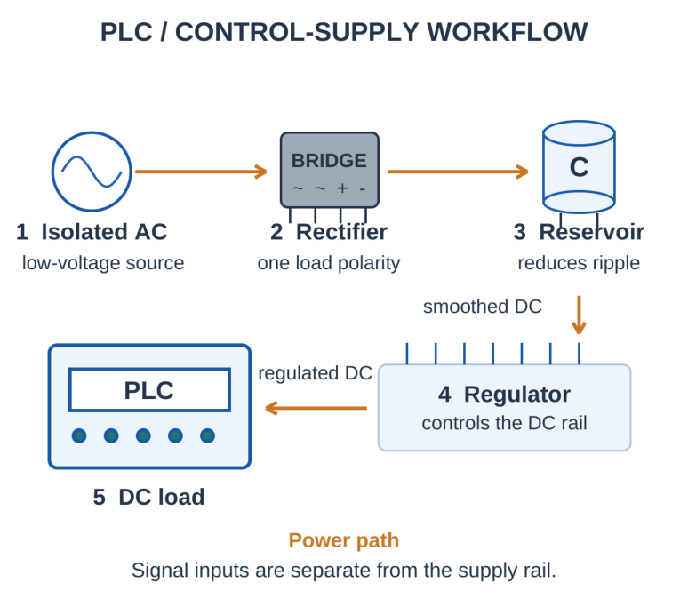
Follow the energy path. An isolated source feeds a bridge, reservoir capacitor and regulating stage. The bridge gives one load-current direction, the capacitor reduces ripple, and the regulator controls output within its operating limits. A packaged switching supply may implement these functions with a different internal topology.
Specify the load. Add the simultaneously active branch currents and consider the stated startup or transient demand. Check the DC voltage at the load terminals, including wiring drop. A supply current rating is a capability; it does not force that current through every connected load.
Select the appropriate regulator. A low-power Zener shunt circuit explains voltage regulation but is not automatically suitable for an entire PLC cabinet. Check current capacity, dissipation, isolation where required and ripple before choosing the actual supply.
Machinery indicator. Use an LED with an appropriate current-limiting element. Check supply and LED-drop extremes, resistance tolerance and resistor power. A lit power indicator proves conditions in its own branch; it does not prove that all machine functions are healthy.
43. [B] CONVEYOR SENSORS AND FIELD INSTRUMENTS
Conveyor detection converts a received-light change into a compatible control signal. Field instruments also need a stable supply at their terminals.
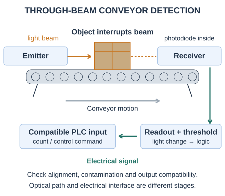
Conveyor sensor sequence. The emitter sends a beam toward the receiver. An object blocks the beam, reducing received light and changing photocurrent. A conditioning stage converts this change into a voltage; a threshold stage forms a defined detection state for the controller. The controller then counts or responds to the object.
Other arrangements. A retro-reflective sensor receives light returned by a separate reflector. A diffuse-reflective sensor receives light reflected by the target itself. The meaning of a high or low output depends on the selected light-on/dark-on setting and output circuit; do not assume that every sensor gives logic 1 when the beam is blocked.
Practical checks. Alignment, contamination, ambient illumination, object transparency and response time affect detection. Match the sensor output type and voltage to the receiving input. Check the common reference or isolation arrangement and the switching threshold.
Field-instrument supply. A pressure, temperature or process instrument requires the specified operating voltage at its terminals, adequate current and acceptable ripple. Supply and measurement signals are different functions, even when a particular interface shares conductors. Follow the stated interface arrangement.
Fault reasoning. Measure the supply at the instrument under load. Ripple can disturb measurements and a voltage valley can cause resets.
A correct no-load voltage does not prove that a supply will remain suitable after cable drop or a load increase. A Zener reference may be useful in a small circuit, but complete instrument power must satisfy the actual power demand.
44. [C] pH METERS, GLUCOMETERS AND DIAGNOSTIC LEDs
A pH meter, glucometer or diagnostic instrument needs a supply with the specified DC voltage, current capability and permissible ripple. Powering the instrument is different from measuring the biological or chemical quantity. A correct no-load voltage alone does not establish a suitable supply.
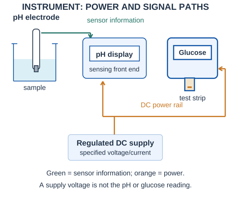
Supply stages. In a low-voltage AC supply, the bridge rectifier produces one load-current direction, the reservoir capacitor smooths the waveform and a regulating stage maintains the intended output within its specified input and load limits. A battery-powered meter may instead use battery conditioning and regulation without an AC rectifier.
pH meter. The electrode produces a measurement-related electrical signal. Its high-impedance sensing front end and the display/control circuits require an appropriate supply. Power-supply ripple or reference instability may introduce error; the supply voltage is not itself the pH reading.
Glucometer. A test strip and its sensing interface produce a glucose-related signal. Signal processing and calibration turn that response into a displayed result. A regulated supply supports consistent circuit operation; it does not directly convert supply voltage into blood-glucose concentration.
Diagnostic indicator LED. An LED can show power or a selected instrument state. Use an appropriate current-limiting resistor, correct polarity and tolerance checks. A lit LED does not prove that the measurement is accurate or that the instrument has completed its self-checks.
Design checks. Account for the simultaneously active load, supply tolerance, ripple valley, wiring drop and regulator dissipation. A small Zener shunt reference is useful for explaining regulation but cannot automatically power an entire instrument. The numerical circuits here are educational supply models.
45. [C] PULSE OXIMETER AND GREENHOUSE LIGHT SENSING
Pulse oximeters detect wavelength-dependent light through tissue; greenhouse sensors monitor environmental light. Both need a suitable photodetector and readout, but their calibration and processing differ.
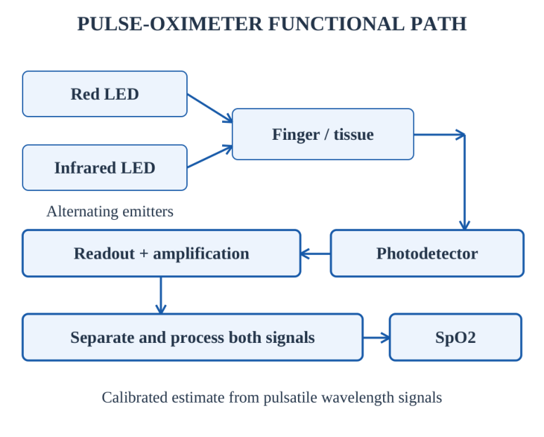
Pulse oximeter: optical path. A transmissive finger probe sends red and infrared light through tissue to a photodetector. The emitters are driven at different times so their responses can be separated. A detector converts received light into an electrical signal, and the readout electronics amplify and process the small changes.
Why two wavelengths? Oxygenated and deoxygenated haemoglobin absorb red and infrared light differently. Pulsatile changes associated with arterial blood are separated from a larger non-pulsatile background. A calibrated relationship involving both wavelength signals is used to estimate peripheral oxygen saturation (SpO2). One raw photodiode voltage is not a direct oxygen percentage.
Signal quality. Motion, ambient light, poor probe placement and weak perfusion can disturb the optical signal. The photodetector is one part of the measurement chain; appropriate emitter timing, signal conditioning and processing are also necessary. This unit covers the functional role, not clinical interpretation.
Greenhouse light monitoring. A photodiode or phototransistor receives light at a representative location. A load or current-to-voltage readout produces an electrical signal; a monitor records it or compares it with a chosen threshold. A controller may then operate supplemental lighting or shading through a suitable driver.
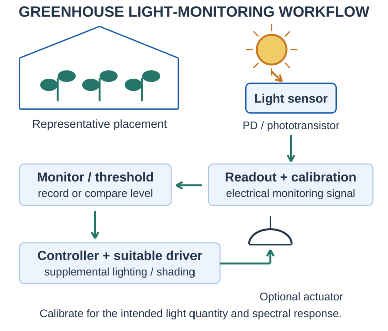
Choose the measured quantity. A general detector response depends on wavelength, angle and the sensor calibration. A raw photocurrent is not automatically lux, solar irradiance or photosynthetic photon flux. Use calibration for the intended quantity and consider whether the sensor spectral response matches the purpose.
Placement and maintenance. Avoid unrepresentative shading, direct glare and contamination. Account for daily variation, condensation and temperature. Check the detector-output range and the receiving circuit. A threshold should correspond to a stated monitoring objective rather than an arbitrary unlabelled voltage.
Application comparison. In a pulse oximeter, the detector helps measure wavelength-dependent transmitted light through tissue. In a greenhouse, the detector monitors environmental light. Both convert light into an electrical response, but their optical arrangements, calibration and processing are different.
46. FORMULA SHEET WITH CONDITIONS
| Quantity | Expression and condition |
|---|---|
| Forward series current | (VS – nVF)/R, valid conducting constant-drop loop |
| Sine peak | Vm = √2 Vs,rms |
| HWR no-filter average / RMS | Vm/π and Vm/2; ideal resistive load |
| Bridge no-filter average / RMS | 2Vm/π and Vm/√2; ideal resistive load |
| Recharge frequency | f for HWR; 2f for bridge |
| Small-ripple voltage | ΔVpp ≈ IL/(frC) |
| Reservoir average / valley | Vpk,out – ΔVpp/2; Vpk,out – ΔVpp |
| Triangular ripple RMS | ΔVpp/(2√3) |
| Zener current | (VS – VZ)/RS – IL, regulating assumption |
| LED resistor | (VS – ΣVF)/I, sufficient voltage headroom |
| Capacitor charge / energy | CV and ½CV² |
| Resistor power | I²R = VI = V²/R |
Conditions are part of the formula
The no-filter rectifier averages, filtered-reservoir averages and regulator outputs describe different circuit states. Most wrong answers in this unit come from combining the formula from one row with the circuit condition from another.
47. EXAM TRICKS AND COMMON ERRORS
State the waveform before applying an RMS or average formula. Input sine values, unfiltered rectified values and capacitor-filtered values are different quantities.
Count the diodes in the conducting path: a bridge has four devices but normally two forward drops in a conducting load path.
Write the ripple frequency next to C. A half-wave reservoir recharges once per source cycle; a full-wave bridge recharges twice.
For ripple estimates, distinguish peak-to-peak ripple from the RMS value of its AC component. State the small-ripple and load-current assumptions.
Test the Zener current before fixing the output at VZ. Check low-input / high-load starvation separately from high-input / low-load dissipation.
For LED design, calculate the resistor voltage first. Select a value that respects the worst-case current limit, then check the actual selected resistance and its power.
Check current direction, terminal reference and voltage margin. Reject a negative current if the assumed conducting diode model permits only forward current.
Use tolerance corners consistently, retain units, and verify the component model and operating state before interpreting the numerical answer.
48. SHORT-ANSWER REVISION
Why is the junction region called depleted?
It has fewer mobile majority carriers than the adjacent neutral regions; the crystal and fixed ionised dopants remain.
Does forward bias uniquely determine current?
No. The external circuit and the selected diode model or actual characteristic determine the operating point.
Why does a bridge keep load polarity unchanged?
The conducting diagonal pair changes with input polarity, while the current direction through the DC load remains the same.
Does a reservoir capacitor regulate voltage?
It reduces variation between charging pulses. A separate regulating mechanism is needed to control voltage across the specified input and load range.
Why test a Zener operating-state assumption?
The input and resistor may not provide enough current for both the load and the required Zener current. The output is then not fixed at the nominal Zener voltage.
Why limit LED current?
The steep forward characteristic makes direct voltage drive sensitive to variation. A resistor or current-regulating driver establishes an appropriate operating current.
Why distinguish a board power input from a GPIO pin?
A power input supplies the board, while a GPIO pin carries a logic signal. A 5 V power input does not make 3.3 V GPIO signals tolerant of a 5 V connection.
Which practical stages must be distinguished?
Rectification, filtering, regulation, current limiting and signal conditioning perform different functions. Identify the actual purpose of each component before choosing a formula.
What does a phototransistor add to light detection?
It provides internal transistor current gain. Speed, linearity and saturation depend on the device and readout circuit.
Why does a conveyor photodiode need an interface?
Its light-dependent current must be converted into a defined, compatible electrical signal before a controller can interpret it.
Why are red and infrared emitters used in a pulse oximeter?
The wavelength responses and their pulsatile components are processed through a calibrated relationship. One raw light voltage is not an oxygen percentage.
Does raw greenhouse photocurrent directly measure plant-useful light?
No. Spectral response, calibration, sensor placement and the intended light quantity must be considered.