
Electronics Unit 3: Operational Amplifiers, Sensors and Signal Conditioning
Subject: Fundamentals of Electronics Engineering
University: AKTU
Course: B.Tech First Year
Semester: I & II
Course Codes: AEC101A / AEC201A | AEC101B / AEC201B | AEC101C / AEC201C
Applicable Streams: CSE, EE, ECE, CE, ME, CH, TX, BT & AG
Unit III Introduction
Operational amplifiers connect small electrical signals to useful measurements and decisions. This combined unit develops ideal and practical amplifier behaviour, then covers industrial, biological and agricultural sensing with calibrated signal conditioning.
Topics Covered
| Topic | Pages |
|---|---|
| Op-amp principles and practical limits | 3–8 |
| Inverting, non-inverting and summing | 8–14 |
| Comparators and A applications | 14–22 |
| Temperature sensors and humidity | 23–25 |
| Strain, LVDT and proximity | 25–27 |
| Bridge and industrial interfaces | 27–29 |
| pH, DO, soil and biopotentials | 28–31 |
| Applications and final revision | 31–33 |
Coverage
All six A/B/C course codes and nine streams. The branch-wise topic guide identifies the prescribed sections. Read the shared foundation, then follow your prescribed application sections.
How to Use These Notes
- Read the branch guide before starting.
- Label amplifier inputs, supplies and signal reference.
- Decide whether feedback is negative and unsaturated.
- Identify the sensor output type and calibration.
- Try each problem before reading the worked answer.
- Check polarity, input range and output headroom.
What Is Included?
| Study Support | Included |
|---|---|
| Worked problems | 50 numbered problems with steps and checks. |
| Labelled figures | Amplifier circuits, feedback and sensing principles. |
| Realistic images | 10 component and application photographs. |
| Dedicated applications | Industrial temperature/pressure, proximity, pH/DO, soil and biopotential signals. |
| Revision | Formula conditions, memory cues and short answers. |
Key Distinction
The virtual-short approximation requires stable negative feedback and linear operation. A comparator deliberately responds to an input difference and generally operates at an output limit.
Numerical Convention
Values are educational assumptions. Retain precision until the final answer. An approximate model is valid only within its stated conditions.
Unit Overview and Branch-Wise Reading Map
Use this map to select your prescribed content. Sections 1–30 establish the op-amp circuits and A-group applications; B/C readers use the relevant non-inverting, comparator and conditioning lessons before their dedicated sensor sections.
| Topics / Application Block | Applicable Branches | Where to Read |
|---|---|---|
| Ideal/practical op-amp, 741, feedback, inverting/non-inverting, follower, summer and comparator | A: CSE, EE, ECE | Sections 1–21 |
| Temperature/light/pressure amplification, night lamp, audio and ECG/EEG concept | A: CSE, EE, ECE | Sections 22–30 |
| Non-inverting gain, comparator and conditioning foundation | B: CE, ME, CH, TX; C: BT, AG | Sections 12–14, 19–21, 31 |
| Thermistor, thermocouple and Wheatstone bridge | B and C groups | Sections 32, 34, 40 |
| PT100, strain/pressure, LVDT and proximity sensors | B: CE, ME, CH, TX | Sections 33, 37–39 |
| 4–20 mA / 0–10 V; reactor, pressure, loom and structural tilt | B: CE, ME, CH, TX | Sections 41, 45 |
| DS18B20, humidity, pH, DO, soil moisture, light and NPK | C: BT, AG | Sections 35–36, 42–43 |
| ECG/EMG conditioning, fermenter and agriculture applications | C: BT, AG | Sections 44, 46 |
| Diagnosis, formula conditions and final revision | All: select your syllabus topics | Sections 47–49 |
Syllabus Groups and Official Unit Names
- A — CSE, EE, ECE: Operational Amplifier (Op-Amp).
- B — CE, ME, CH, TX: Sensors, Transducers, and Signal Conditioning.
- C — BT, AG: Sensors, Biosensors, and Signal Conditioning.
What Is Included
50 numbered solved problems, 10 realistic component/laboratory images, labelled circuits and sensor illustrations. Both semester codes within each group have the same unit syllabus. Extra A-only amplifier detail is enrichment for B/C, not an additional prescribed requirement.
Reading rule: Identify the sensing principle, electrical output, conditioning and calibration. Course-specific [B] and [C] labels distinguish dedicated lessons. Numerical values are stated educational assumptions.
1. What an Operational Amplifier Does
An operational amplifier is a high-gain, direct-coupled differential voltage amplifier. It responds to the difference between two input voltages and obtains output energy from its power supply. External feedback determines the useful closed-loop operation. Its name comes from analog mathematical operations such as addition, subtraction and scaling.
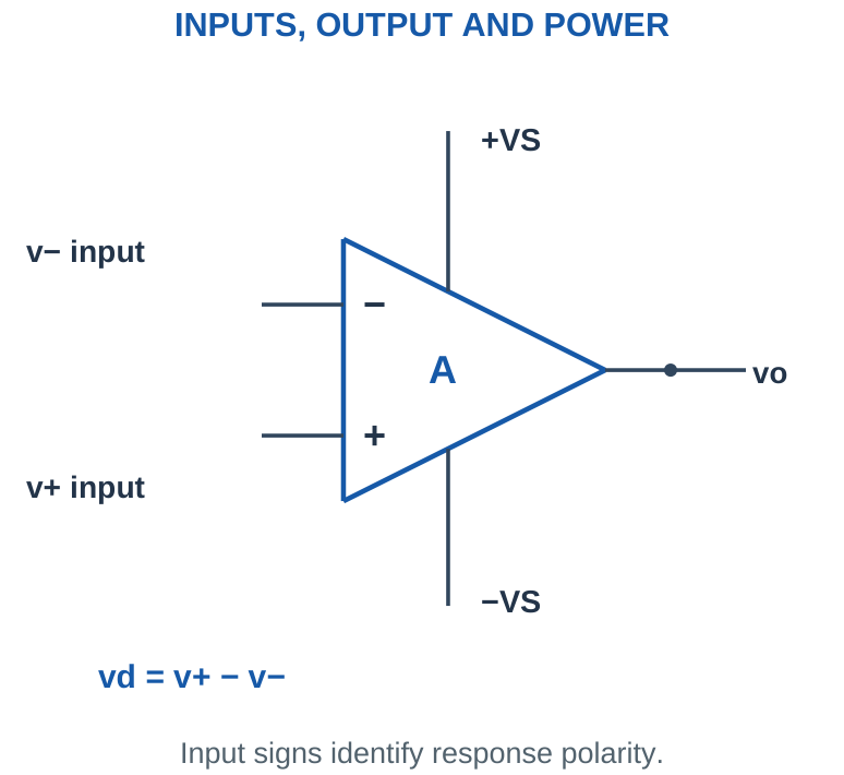
Signal and supply references: The non-inverting input is marked + and the inverting input is marked -. These signs describe the direction of the output response to a change at either input; they do not prescribe whether either input must be positive or negative relative to ground. Define vd = v+ – v-. In the unsaturated open-loop model, vo = AOL vd.
| Quantity | Meaning |
|---|---|
| v+, v- | Input node voltages measured from the reference |
| vd | Differential input v+ – v- |
| AOL | Open-loop differential voltage gain |
| +VS, -VS | Positive and negative supply nodes |
| vo | Output node voltage from the reference |
Essential habit: Write the supply arrangement and output limits before calculating a large output. A predicted 100 V output from an amplifier powered by ±15 V is not physically available.
Worked Problem 3.1: Differential Input and Requested Output
Problem: v+ = 0.99997 V, v- = 1 V and AOL = 100000 V/V. The permitted output range is ±12 V. Find vd and vo.
Model / approach: Use signed input difference, then check the output range.
Step 1: vd = v+ – v- = -30 µV.
Step 2: vo,requested = AOL vd = -3 V. This lies inside ±12 V.
Answer: vo = -3 V in the stated unsaturated model.
Check and interpretation: The common input voltage is close to the larger input values, while the differential voltage is only a few microvolts. A practical device must support that common-mode level; it is not found by subtracting the inputs.
2. Ideal Characteristics and Useful Approximations
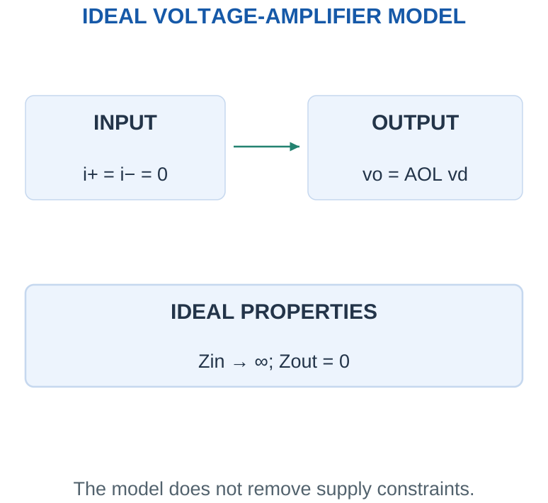
The ideal op-amp is a mathematical model that makes introductory circuit analysis manageable. It has infinite differential gain and input impedance, zero output impedance, infinite bandwidth and slew rate, zero input offset voltage and zero input bias currents. A real device approaches only some of these properties over a limited operating range.
Meaning of the Three Main Ideal Properties
Infinite input impedance: Neither input draws current, so i+ = i- = 0. Current through an external resistor connected to an input may still flow through another external branch.
Zero output impedance: The ideal output voltage does not change with load current. A real amplifier has output resistance and finite current capability.
Infinite gain: A finite linear output requires the differential input to approach zero when stable negative feedback acts.
The ideal model does not remove Kirchhoff’s laws, resistor dissipation or the need for a supply. Infinite bandwidth and slew rate are additional idealisations; they are not true properties of a 741.
Exam trick: Separate input current from output current. “No input current” does not mean “no current anywhere in the op-amp circuit”.
3. Open-Loop Gain, Polarity and Saturation
An open-loop circuit has no external path forcing the output back toward an input condition. Its enormous gain means that a tiny differential input can request an output beyond the available swing. The output then approaches a limiting level instead of continuing to follow AOL vd.
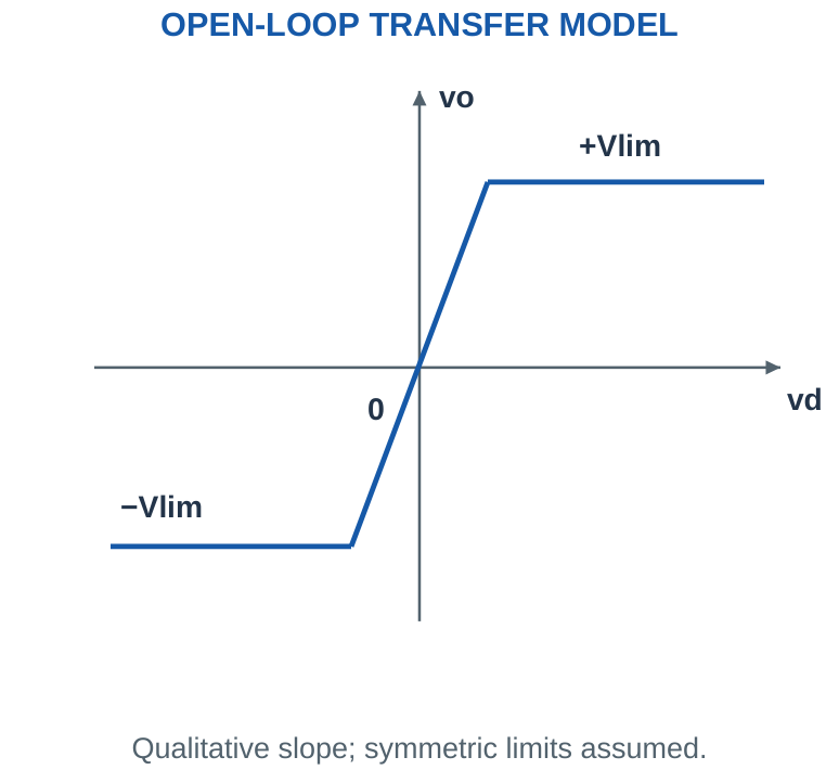
A practical calculation sequence: First find vd with its sign. Next calculate the linear request AOL vd. Finally compare that request with the given high and low output limits. Use the appropriate limit if necessary. At vd = 0, an ideal model gives zero; a practical open-loop circuit may select a limit because of offset and noise.
Do not use v+ = v- to solve an open-loop comparator. The inputs are imposed by the sources, and the amplifier normally cannot move them. An open-loop response can be useful for a decision, but it is usually unsuitable for accurate linear sensor amplification.
Unit conversion: A gain of 200 V/mV means 200,000 V/V. A differential input of 50 µV is 0.000050 V, not 0.05 V.
Worked Problem 3.2: Apply the Output Limit
Problem: An open-loop model has vd = 100 µV, AOL = 200000, and output limits ±12 V. Find the output.
Model / approach: Calculate the linear request before selecting a permitted limit.
Step 1: vd = 0.0001 V. The linear request is 20 V.
Step 2: Compare with -12 V and +12 V: the model gives 12 V.
Answer: vo = 12 V; the output is limited.
Check and interpretation: A saturated output is not equal to AOL vd once the request exceeds the allowed swing. Neither input is automatically forced to match the other in this open-loop circuit.
4. Negative Feedback and the Virtual Short
Negative feedback returns a portion of the output in a direction that opposes the original differential error. If the output rises too far in a normal non-inverting stage, the fed-back inverting voltage rises and reduces vd. The resulting closed-loop gain is mainly determined by the external resistor network.
Worked check: Recognise the virtual short
A correctly connected non-inverting stage has vin = 0.4 V and gain 5. The requested output is 2 V. Its feedback fraction is 1/5, giving v- = 0.4 V. The two inputs agree because the loop regulates the divider voltage, while both are above ground. Equal inputs therefore do not necessarily mean a virtual ground.
Worked check: Loss of headroom breaks the rule
Suppose gain 10 requests 20 V from a 2 V input, but the output limit is 12 V. The feedback fraction is 0.1, so the divider only returns 1.2 V. The difference is 2 – 1.2 = 0.8 V. The output is saturated, and imposing equal inputs would hide the failed operating assumption.
Worked check: Sign of feedback
In a non-inverting stage, a rise in vo raises v- through the divider. This reduces v+ – v- and opposes the original rise. A return to v+ instead reinforces the rise and cannot be analysed by blindly applying the same linear equal-input rule.
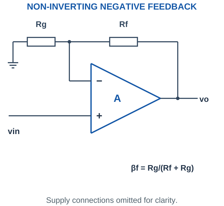
Two rules, with conditions: For an ideal op-amp with stable negative feedback, linear operation and valid input/output ranges, use i+ = i- = 0 and v+ ≈ v-. The latter is a virtual short: equal or nearly equal voltages without a physical wire between the input pins. It does not permit current to flow through the input pair.
If the non-inverting input is at zero, the inverting node may be a virtual ground. It has approximately zero voltage because feedback regulates it. It is not a separate ground connection capable of supplying arbitrary current. When the output saturates, the feedback cannot preserve this condition.
Check before applying: Trace the output connection. A path to the + input may create positive feedback; the virtual-short rule is not justified simply because any feedback wire exists.
Worked Problem 3.3: Residual Virtual-Short Error
Problem: A linear feedback stage produces vo = 5 V with AOL = 200000. Find v+ – v-.
Model / approach: Use the finite open-loop relationship at the stated operating point.
Step 1: vd = vo/AOL = 5/200000 = 25 µV.
Step 2: The small nonzero difference supports the large finite gain. It is not a wire connection between the inputs.
Answer: vd = 25 µV.
Check and interpretation: The equal-input rule is an approximation. The sign of the differential error follows the output sign when AOL is positive; the operating point must still remain in the linear region.
5. Finite Gain and Closed-Loop Accuracy
Real open-loop gain is large but finite. For a non-inverting feedback network with fraction βf, vo = AOL(vin – βf vo), giving Acl = AOL/(1 + AOL βf). When AOL βf is much greater than one, Acl approaches 1/βf. The difference between the input pins remains vo/AOL.
Use the right approximation: The ideal gain is a design target, not a promise of exact performance. Finite open-loop gain, resistor tolerance, input offset, bias currents, frequency response and loading can all cause an error. Do not add unrelated typical errors as if they were guaranteed worst-case specifications.
For the inverting circuit, the ideal signal gain is -Rf/Rin but its noise gain is 1 + Rf/Rin. Noise gain describes the amplification of a small equivalent input offset voltage and is also useful in the elementary bandwidth estimate. Keeping these two gains distinct prevents several common numerical mistakes.
Quick estimate: For large loop gain, fractional closed-loop error is approximately 1/(AOL βf). Use the full expression when the question asks for a precise finite-gain value.
6. IC 741 Pin Diagram and Supply Wiring
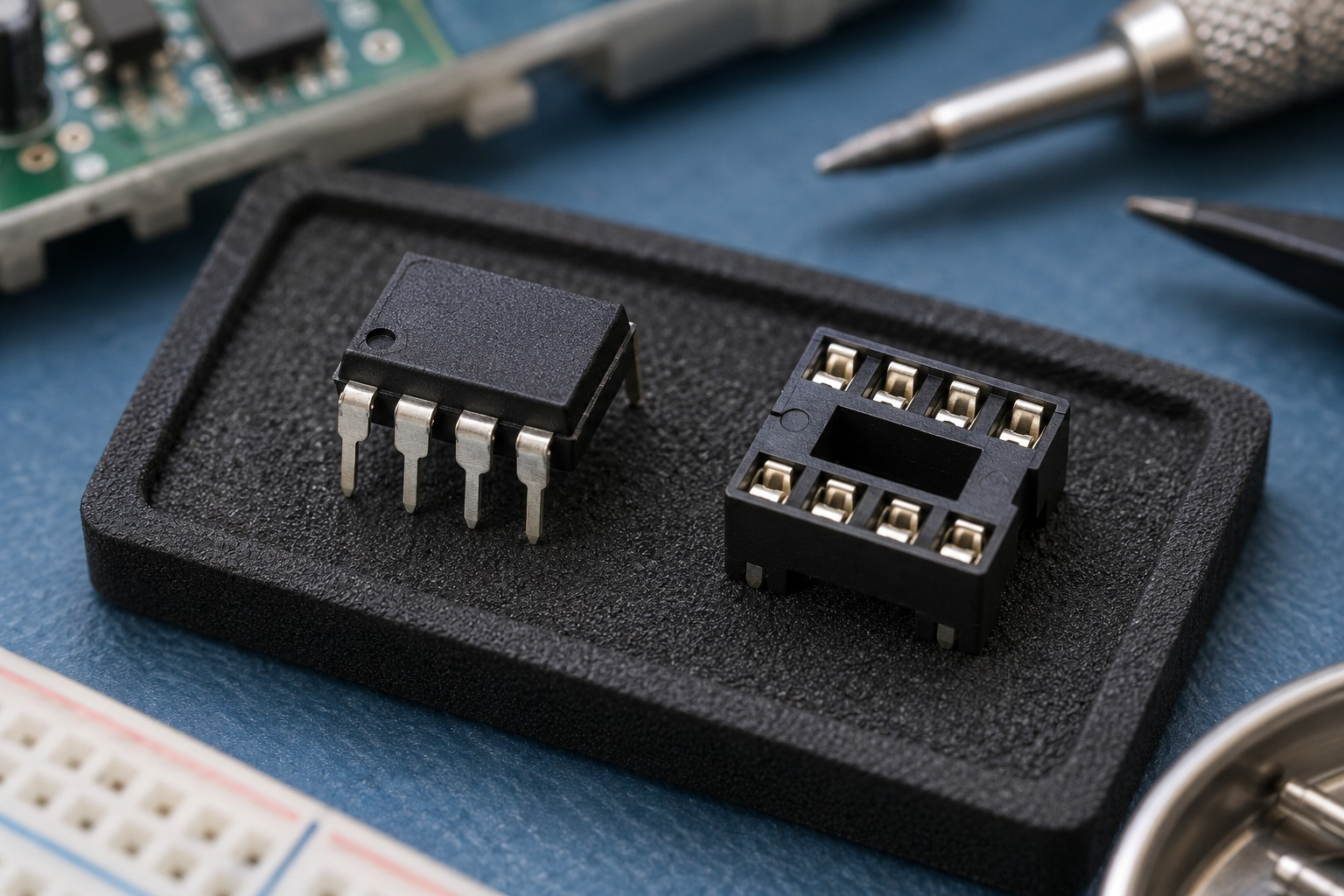
The 741 is a classic bipolar general-purpose op-amp. Its eight-pin DIP is read from the top view, using the notch or dot to locate pin 1. Pin numbering goes counterclockwise around the package. A pin diagram is a package connection map, not the internal circuit or the triangle symbol.
LINEAR FEEDBACK CHECK
- Negative feedback is present.
- Requested output fits the allowed swing.
- Both inputs satisfy common-mode limits.
- Current, bandwidth and slew demand remain valid.
Only then use v+ approximately equal to v-. The inputs are not physically shorted.
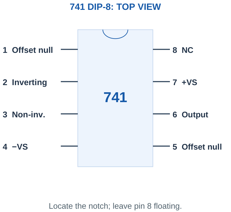
| Pin | Function |
|---|---|
| 1 and 5 | Offset null |
| 2 | Inverting input |
| 3 | Non-inverting input |
| 4 | Negative supply |
| 6 | Output |
| 7 | Positive supply |
| 8 | No connection |
Dual supplies and reference: With ±15 V supplies, pin 7 is +15 V, pin 4 is -15 V and the midpoint is the 0 V reference. The voltage between the supply pins is 30 V. Grounding pin 4 instead creates a single-supply arrangement; it does not magically provide a negative rail. Use appropriate local supply bypassing in a physical circuit.
Pin memory cue: 2 is minus input, 3 is plus input, 4 is minus supply, 6 is output, 7 is plus supply. Never infer a supply pin from the location of the + input symbol.
Worked Problem 3.4: Supply-Pin Voltages
Problem: A 741 DIP has pin 7 at +15 V and pin 4 at -15 V relative to ground. Pin 3 is at 0.2 V. Find voltage between supply pins and identify pin 3.
Model / approach: Separate supply voltage from signal voltage.
Step 1: V7 – V4 = 15 – (-15) = 30 V.
Step 2: Pin 3 is the non-inverting signal input; its 0.2 V is not a supply rail.
Answer: 30 V between supplies; pin 3 is the + input.
Check and interpretation: The output swing is not automatically 30 V peak-to-peak. Available swing needs its own device and load conditions.
7. Practical 741 Characteristics
A 741 is not a rail-to-rail, zero-offset or high-speed ideal device. Representative LM741 figures include open-loop gain around 200,000 V/V, input bias current around 80 nA and slew rate around 0.5 V/µs under the relevant typical test conditions. These are illustrative typical values, not universal limits for every manufacturer, grade or temperature.
Worked check: Typical is not a limit
If an exercise gives 80 nA bias current and a 100 kΩ source resistance, the associated voltage drop is 80 nA × 100 kΩ = 8 mV. This is a nominal model result. It is not a worst-case specification unless the supplied current is explicitly a guaranteed maximum under the required conditions.
Worked check: Input and output ranges differ
With an assumed input common-mode range ±10 V and output swing ±12 V, a follower input of 11 V requests an apparently acceptable 11 V output. The input check nevertheless fails. Output headroom alone cannot validate the follower. A different gain formula does not enlarge the input range of the selected device.
Parameters that matter: Input offset voltage is the small differential voltage needed to balance the output. Input bias current is the average of the magnitudes of the two input currents; offset current describes their mismatch. Finite input resistance loads a high-resistance source. Output swing depends on load and available supply voltage. A typical short-circuit current figure is not a recommended load-current rating.
| Property | Ideal | Practical Consequence |
|---|---|---|
| Input impedance | Infinite | High-resistance sensors can be loaded |
| Output impedance | Zero | Load changes can introduce error |
| Offset and bias | Zero | DC output error appears |
| Speed | Unlimited | Bandwidth and slew limits apply |
| Voltage range | Unrestricted model | Input range and output headroom matter |
Design interpretation: Do not assume a classic 741 works from a 0–5 V supply or senses inputs at its supply rails. A low-voltage sensor design may need a different op-amp selected for those conditions.
8. Offset Voltage, Bias Current and Balancing
Even with the intended signal set to zero, a real amplifier can produce a nonzero output. Input offset voltage behaves approximately like a small differential error voltage. In a closed-loop stage, its output contribution is approximately noise gain × VOS, provided the output remains linear. The polarity of an unknown offset is not predictable from its magnitude alone.
Worked check: Output-error polarity
A noise gain of 6 and offset magnitude 1 mV give an output-error magnitude about 6 mV. Without an offset sign, report ±6 mV as a possible signed contribution or state the magnitude explicitly. An unknown positive-or-negative error should not be silently added as a known positive output voltage.
Worked check: Bias-current mismatch
After ideal resistance balancing, a supplied mismatch current of 10 nA acting through 100 kΩ gives an approximate residual output-error magnitude 1 mV. This simplified residual model does not also remove VOS. If VOS is 1 mV and noise gain is 11, its separate output-error magnitude is about 11 mV.
Bias compensation principle: For an inverting amplifier whose input source becomes ground at DC, choose Rb ≈ Rin || Rf. Equal bias currents then develop similar input-node errors and their principal effects tend to cancel. Input offset-current mismatch, resistor tolerance, source resistance and VOS leave residual error. Recompute the resistance if the source has appreciable DC resistance.
Pins 1 and 5 allow offset adjustment using the correct device arrangement. They are not extra signal inputs. Offset adjustment at one condition does not remove all temperature drift or make the device ideal.
Numerical trap: An inverting stage with signal gain -10 has noise gain 11. A 2 mV offset produces an output-error magnitude of about 22 mV, not 20 mV.
Worked Problem 3.5: Offset Uses Noise Gain
Problem: An inverting stage has Rf/Rin = 10 and an equivalent input offset magnitude 2 mV. Estimate output offset magnitude, ignoring bias currents.
Model / approach: Multiply the offset by noise gain, not by the signal-gain magnitude.
Step 1: Signal gain = -10; noise gain = 1 + 10 = 11.
Step 2: |vo,error| ≈ 11 × 2 mV = 22 mV.
Answer: Estimated output offset magnitude = 22 mV.
Check and interpretation: The actual offset polarity is unspecified. This approximation assumes the resulting operating point remains linear and treats offset as an equivalent small input voltage.
9. Inverting Amplifier: Derivation and Circuit
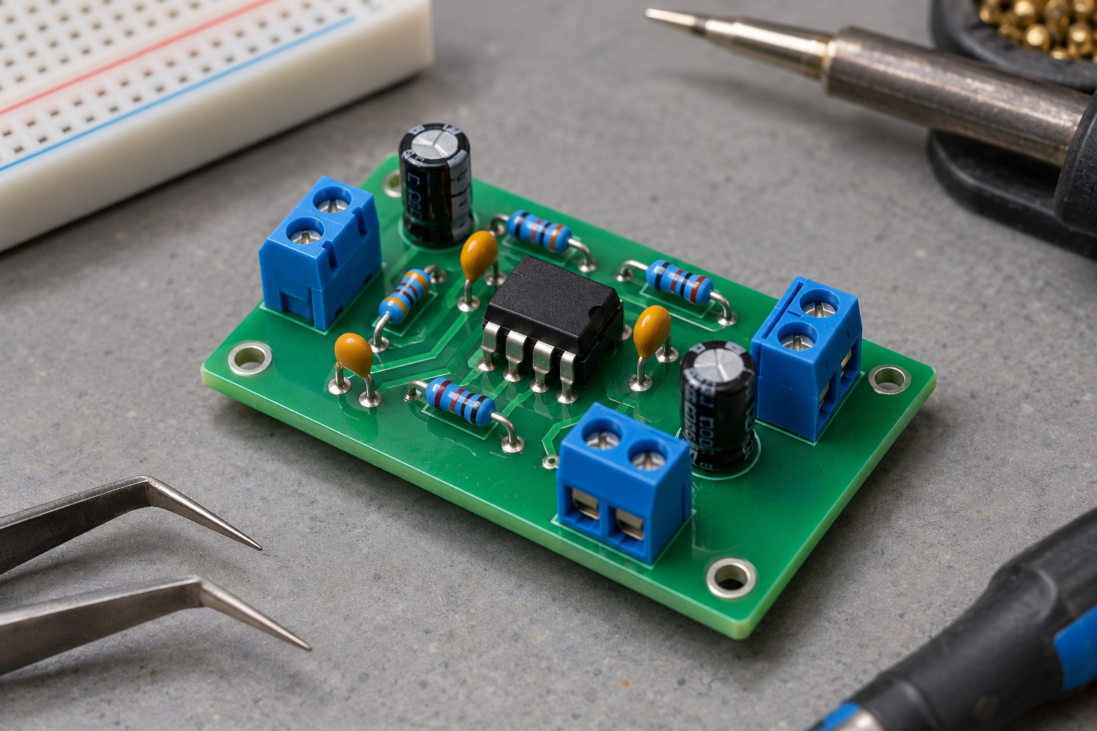
The signal reaches the inverting node through Rin. The non-inverting input is grounded, and Rf connects the output to the inverting node. Assuming valid linear negative feedback, the inverting node is at virtual ground and no current enters the input pin.
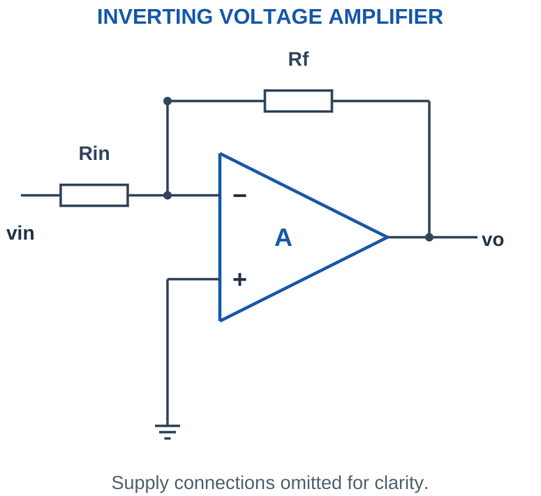
Gain from KCL: Input-resistor current is (vin – 0)/Rin. Feedback-resistor current from the node toward the output is (0 – vo)/Rf. Equating them gives vo = -(Rf/Rin)vin. The minus sign indicates polarity reversal for a DC input and a 180° phase inversion for a sinusoid in the useful frequency range.
| Relationship | Condition |
|---|---|
| Av = -Rf/Rin | Ideal linear negative feedback |
| Zin seen by source ≈ Rin | Summing node held near ground |
| iin = vin/Rin | Grounded non-inverting input |
| Noise gain = 1 + Rf/Rin | Equivalent input-error amplification |
The source sees Rin rather than the op-amp’s extremely high bare input impedance. A source with resistance Rs adds a series voltage drop and changes the gain from its internal voltage to -Rf/(Rs + Rin).
Worked Problem 3.6: Inverting Gain, Current and Output
Problem: Rin = 10000 Ω, Rf = 100000 Ω and vin = 0.2 V. The + input is grounded. Permitted output is ±12 V. Find gain, output and input current.
Model / approach: Use virtual ground only after assuming valid linear negative feedback.
Step 1: Av = -Rf/Rin = -10.
Step 2: vo = Av vin = -2 V. The request fits ±12 V.
Step 3: Iin = vin/Rin = 20 µA; If toward output has the same signed value.
Answer: Av = -10; vo = -2 V; Iin = 20 µA.
Check and interpretation: The voltage at the input node is approximately zero while the source voltage is not. Use the resistor drop, not the input pin voltage alone, when calculating source current.
10. Inverting Design, Tolerances and Clipping
Choose the desired gain magnitude, then select a sensible Rin and calculate Rf = |Av| Rin. Very low resistances demand output and source current. Very high resistances increase bias-current error and susceptibility to interference. There is no one perfect resistance value for every application.
Worked check: Source resistance changes signal gain
An internal source voltage drives 2 kΩ series resistance followed by Rin = 8 kΩ. With Rf = 50 kΩ, the gain from the internal source is -50/(2 + 8) = -5. For 0.2 V, output is -1 V. The gain -6.25 applies from the external input terminal before Rin, not from the source’s internal voltage.
Worked check: Asymmetric input endpoints
Gain -4 maps vin = -1 V to +4 V and vin = +2 V to -8 V. Both fit a stated ±10 V swing. Checking only the smaller 1 V magnitude would overlook the larger negative output demand. Evaluate the endpoints with their signs before describing the complete range.
Output headroom check: Calculate the complete requested output range from the complete input range. For a zero-centred input with peak Vp and symmetric permitted swing ±Vlim, require |Av| Vp ≤ Vlim. For a DC offset plus an AC input, check both upper and lower peaks separately. Use the given permitted output swing, not automatically the supply voltage.
For independent resistor tolerances, maximum gain magnitude occurs at Rf,max/Rin,min and minimum gain magnitude at Rf,min/Rin,max. A nearest standard resistor is acceptable only if the actual gain and limits still meet the requirement.
Exam trick: A negative output is normal on a suitable dual supply. It is not evidence of a wrong answer. On a single supply, a requested negative output usually signals the need for a biased reference or a revised circuit.
Worked Problem 3.7: Gain Design and Maximum Input Peak
Problem: Design an inverting magnitude gain 10 using Rin = 10000 Ω. Output swing is limited to ±12 V. Check a zero-centred input peak of 1.5 V.
Model / approach: Calculate Rf and compare both requested peaks with the symmetric swing.
Step 1: Rf = 10 × 10000 = 100000 Ω.
Step 2: Maximum linear input peak = 12/10 = 1.2 V.
Step 3: Test output peak magnitude = 10 × 1.5 = 15 V; this exceeds the limit.
Answer: Rf = 100000 Ω; allowed input peak ≤ 1.2 V. The tested signal clips.
Check and interpretation: An amplitude check is not a speed or current check. A signal that fits the swing can still exceed bandwidth or slew capability at a sufficiently high frequency.
11. Inverting Amplifier with a Reference
If the non-inverting input is held at Vref, feedback holds the inverting node near Vref. The input current becomes (vin – Vref)/Rin. The output must accommodate this current through Rf while maintaining the summing-node voltage.
KCL gives vo = (1 + Rf/Rin)Vref – (Rf/Rin)vin. This is especially useful for translating a sensor range. For example, with Rf/Rin = 2, the slope is -2 while the intercept is 3Vref. The intercept is not merely Vref unless the rest of the topology makes it so.
A mid-supply reference is often called a virtual ground in single-supply signal processing. Distinguish this reference source from an inverting amplifier’s virtual-ground input node. A divider alone has finite resistance and may need buffering; the output-current path still returns through the real supply system.
Range check: Check the common-mode voltage at both op-amp inputs, which is close to Vref here. Also check the requested output endpoints against the actual available swing.
Worked Problem 3.8: Reference Shifts an Inverting Transfer
Problem: Rf/Rin = 2, Vref = 2 V, and vin ranges from 1 to 3 V. Allowed output is 0.5–10 V with a suitable amplifier. Find the requested endpoints and check them.
Model / approach: Use vo = (1 + r)Vref – r vin.
Step 1: Intercept = (1 + 2) × 2 = 6 V.
Step 2: At vin = 1 V, vo = 4 V; at vin = 3 V, vo = 0 V.
Answer: Output endpoints: 4 V and 0 V. At least one fails the stated swing.
Check and interpretation: The first endpoint is larger because this transfer has negative slope. Check the input common-mode level near Vref as well; the specified output range does not establish the input range.
12. Non-Inverting Amplifier
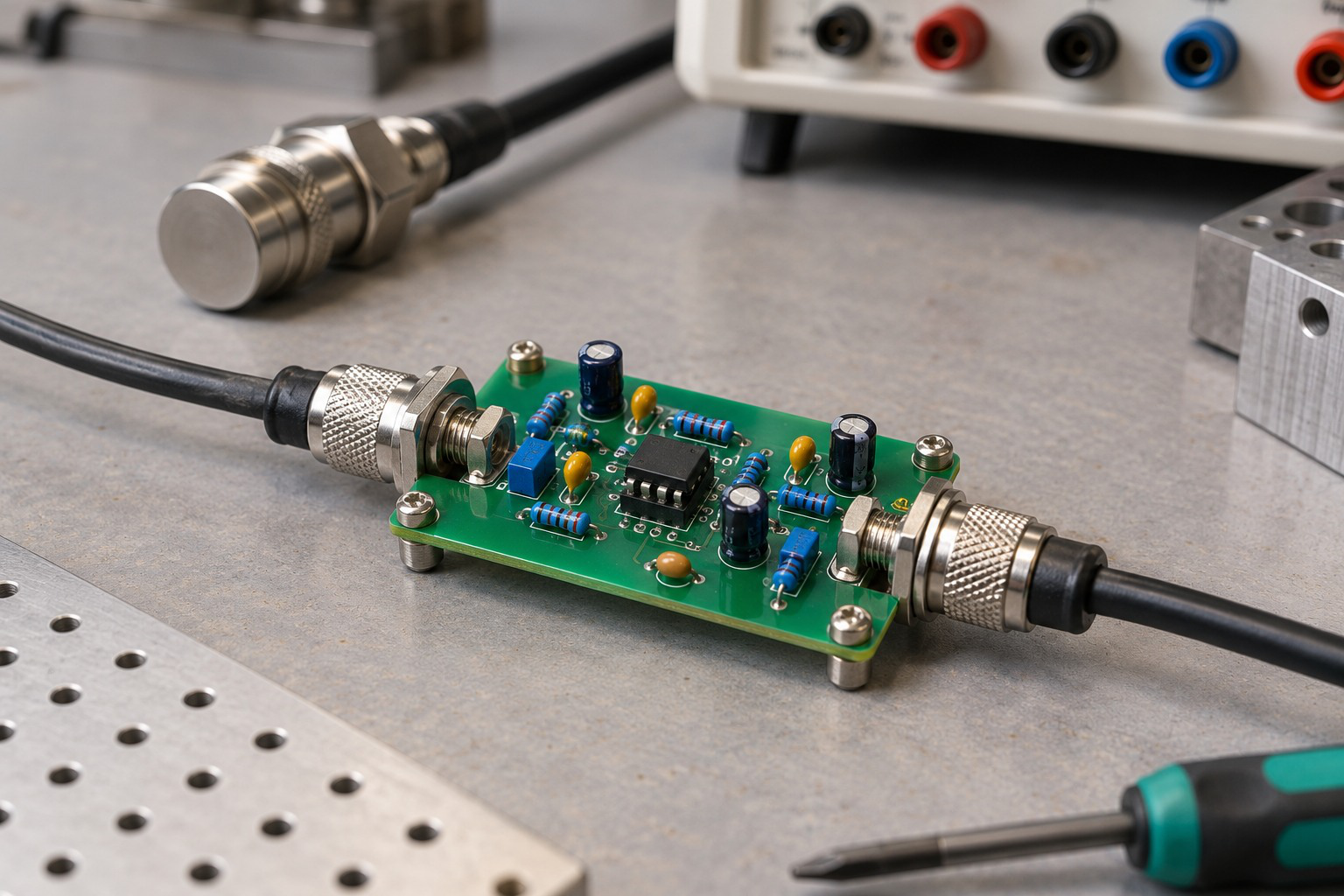
Apply the signal directly to the + input. Connect Rf from output to – input and Rg from the – input to ground. With ideal input current zero, the two resistors form a divider: v- = vo Rg/(Rf + Rg). Feedback sets v- ≈ vin.
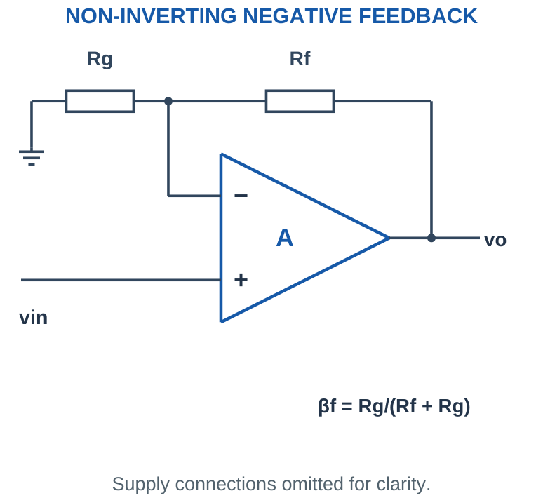
Rearranging gives Av = 1 + Rf/Rg. The output has the same polarity as the input. The source ideally sees infinite impedance at the + input, making this configuration useful when loading should be small. In practice input resistance, bias current and common-mode range remain relevant.
The gain with ordinary positive resistors is at least one. A request for a positive gain of 0.5 cannot be met by choosing a negative resistor in this formula; use an attenuator followed by a buffer or another suitable arrangement.
Common error: Rf/Rg is only the amount by which the non-inverting gain exceeds one. For a gain of 11, choose Rf/Rg = 10, not 11.
Worked Problem 3.9: Non-Inverting Gain and Divider Voltage
Problem: Rg = 10000 Ω, Rf = 90000 Ω and vin = 0.2 V. The output limits are ±12 V. Find Av, vo and v-.
Model / approach: Use ideal linear feedback and the feedback divider.
Step 1: Av = 1 + 90000/10000 = 10.
Step 2: vo = 10 × 0.2 = 2 V, inside the specified limits.
Step 3: v- = vo Rg/(Rf + Rg) = 0.2 V, matching v+.
Answer: Av = 10; vo = 2 V; v- ≈ 0.2 V.
Check and interpretation: The + and – input voltages are nearly equal because the feedback acts in its linear range. They are not generally zero, so this node is a virtual short but not a virtual ground.
13. Non-Inverting Design and Loading Comparison
The non-inverting configuration provides high input impedance, but it does not guarantee unlimited output current. The feedback divider itself draws current from the output, and an external load adds another current demand. Check the sum of the feedback-path and load currents at the output peak.
Worked check: Tolerance includes the added one
For a non-inverting stage, Rf = 90 kΩ and Rg = 10 kΩ with independent ±1% tolerances give Gmin = 1 + 89.1/10.1 = 9.8218 and Gmax = 1 + 90.9/9.9 = 10.1818. Include the added one after forming the ratio.
Resistor and endpoint checks: For a required gain G, use Rf = (G – 1)Rg. Once actual values are chosen, recompute the gain and output endpoints. If the source has a DC offset, the amplifier multiplies it as well as the desired change. A large offset can consume headroom before the useful signal is amplified.
For independent tolerances, Gmax = 1 + Rf,max/Rg,min and Gmin = 1 + Rf,min/Rg,max. This differs from simply attaching the resistor tolerance directly to the final gain number. Check both the gain tolerance and the output-range requirements.
Selection clue: Use a non-inverting stage when positive voltage gain and low source loading are required. Use an inverting stage when negative gain, a summing node or a deliberately defined input resistance is useful.
Worked Problem 3.10: Choose Feedback Resistance
Problem: Required non-inverting gain is 11, Rg = 10000 Ω and test input is 0.3 V. Find Rf and nominal output. Assume a permitted ±12 V output.
Model / approach: Subtract one from the requested gain before setting the resistor ratio.
Step 1: Rf/Rg = G – 1 = 10.
Step 2: Rf = 10 × 10000 = 100000 Ω.
Step 3: vo = 11 × 0.3 = 3.3 V.
Answer: Rf = 100000 Ω; vo = 3.3 V.
Check and interpretation: The test output fits the stated swing. Other input endpoints, resistor tolerances and the device’s common-mode and speed limits remain separate design checks.
14. Voltage Follower and Impedance Isolation
A voltage follower connects output directly to the inverting input and applies the signal to the non-inverting input. It is the unity-gain form of a non-inverting amplifier. Negative feedback makes vo ≈ vin while providing high input impedance and low closed-loop output impedance.
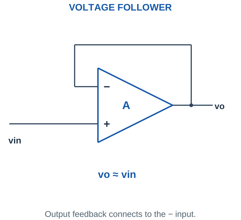
Why unity gain is useful: A sensor may generate the right voltage but have too much internal resistance to drive the next circuit. Direct loading creates a divider and reduces the measured voltage. A suitable follower draws little source current and supplies load current from its own power rails. Its voltage gain is one, but its current and power gain can be substantial.
The follower still requires a device stable at unity noise gain and compatible with the input common-mode voltage, output swing and load. It does not restore a voltage already lost before its input. A large capacitive load can affect stability and may need a device-specific solution.
Misconception: A buffer is not a source of free power. Its load energy comes from the amplifier supply; the source controls the output voltage.
Worked Problem 3.11: Direct Loading Versus Ideal Buffer
Problem: A source has internal voltage 2 V and series resistance 10000 Ω. The load is 10000 Ω. Compare direct connection with an ideal powered follower and find buffered load current.
Model / approach: Direct connection is a divider; an ideal follower isolates the source.
Step 1: Direct load voltage = 2 × 10000/(10000 + 10000) = 1 V.
Step 2: Buffered output = 2 V; load current = 2/10000 = 0.2 mA.
Answer: Direct: 1 V; buffered: 2 V; IL = 0.2 mA.
Check and interpretation: The ideal buffer draws zero source current and supplies the load from its power rails. A real follower must support the resulting input voltage, output swing and current.
15. Inverting Summing Amplifier
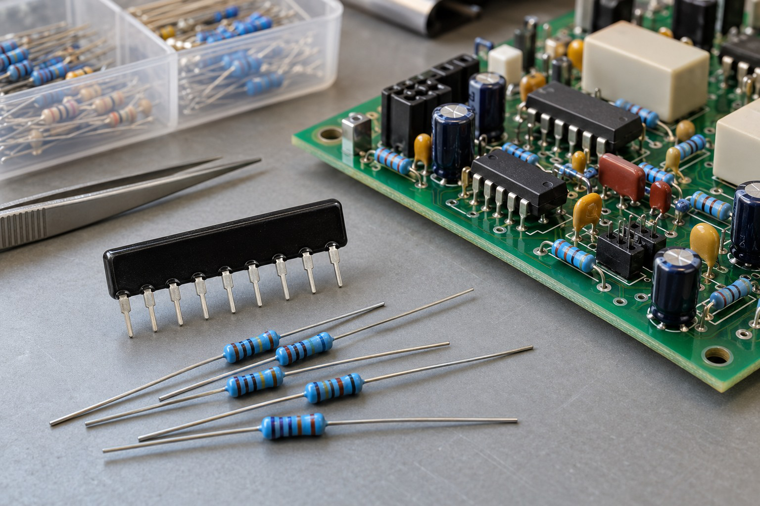
Several input resistors meet at the inverting summing node. Each source contributes a current, and the feedback resistor carries their algebraic sum. With the + input grounded, the node remains near zero during valid linear operation.
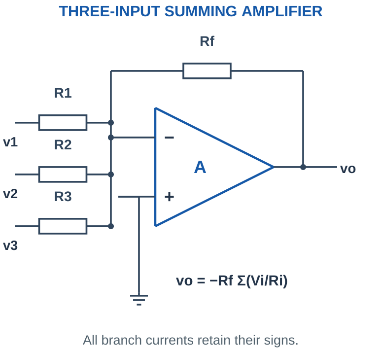
KCL gives vo = -Rf(v1/R1 + v2/R2 + v3/R3). For equal input resistors R, vo = -(Rf/R)(v1 + v2 + v3). Negative input voltages contribute negative currents and may reduce or reverse the total. Do not add only absolute magnitudes.
The sources do not ideally drive each other through the node because feedback holds it near a fixed potential. However, each source is loaded by its own input resistor, and the output must supply the feedback current. Saturation breaks the virtual-ground assumption.
Method: Calculate each signed current first, add the currents, and multiply by -Rf. This is safer than combining differently weighted voltages mentally.
Worked Problem 3.12: Signed Current Summation
Problem: v1, v2, v3 = [0.1, 0.2, 0.3] V respectively; R1, R2, R3 = [10000, 10000, 10000] Ω respectively; Rf = 10000 Ω. Find the output with grounded + input and ±12 V allowed swing.
Model / approach: Use vo = -Rf Σ(Vi/Ri), retaining every sign.
Step 1: Branch currents = 10, 20, 30 µA.
Step 2: Total current toward the node = 60 µA.
Step 3: vo = -10000 × 6 × 10^-5 = -0.6 V.
Answer: vo = -0.6 V.
Check and interpretation: The stated output is within ±12 V. A negative branch current opposes positive branch currents. Adding only voltage magnitudes would give the wrong result for mixed-polarity inputs.
16. Weighted Addition, Averaging and Mixing
Choose different input resistors to apply different weights. A smaller input resistor produces a larger contribution for the same source voltage. Weighted summing supports simple audio mixing, sensor combination and analog arithmetic.
Average versus sum: For n inputs with equal resistor R, choose Rf = R/n to obtain the negative arithmetic mean: vo = -(v1 + … + vn)/n. If Rf = R, the circuit produces the negative sum rather than the average. A second unity inverter can restore positive polarity when the extra stage is justified.
A mixer design must check the worst allowed combination of inputs, not only one input at a time. If all signals can peak with the same sign, the output demand adds. Different phases may reduce a particular instantaneous value but cannot be assumed without information.
Design trap: A binary-weighted summer illustrates conversion of weighted logic levels into analog voltage. Real digital-to-analog conversion also depends on switch resistance, reference accuracy and resistor matching; the ideal summer alone does not guarantee converter accuracy.
Worked Problem 3.13: Weighted Design from Coefficients
Problem: Design vo = -(2v1 + v2 + 0.5v3) with Rf = 20 kΩ. Find the three input resistors and output for v1 = 0.3 V, v2 = 0.4 V and v3 = 0.2 V.
Model / approach: Each coefficient is Rf/Ri.
Step 1: R1 = 20/2 = 10 kΩ; R2 = 20/1 = 20 kΩ; R3 = 20/0.5 = 40 kΩ.
Step 2: vo = -(0.6 + 0.4 + 0.1) = -1.1 V.
Answer: R1 = 10 kΩ, R2 = 20 kΩ, R3 = 40 kΩ; vo = -1.1 V.
Check and interpretation: The largest coefficient uses the smallest resistor. Check the worst allowed simultaneous input combination before choosing output headroom.
17. Differential Amplifier
A differential amplifier responds to the difference between two input signals. In the four-resistor arrangement, v1 enters the – input through R1 and R2 provides feedback; v2 reaches the + input through R3 with R4 from that node to ground.
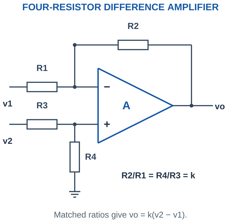
If R2/R1 = R4/R3 = k, the ideal output is vo = k(v2 – v1). The common voltage component ideally cancels. For unmatched ratios, first calculate v+ = v2 R4/(R3 + R4), then vo = (1 + R2/R1)v+ – (R2/R1)v1.
This circuit has finite input resistances determined by its network; it is not automatically an instrumentation amplifier. Sources with unequal or high internal resistance can disturb the effective ratios and loading. For delicate differential sensors, buffered or integrated instrumentation arrangements may be more suitable.
Polarity check: If v2 rises while v1 stays fixed, the output rises. If v1 rises alone, the output falls. This check often catches a reversed subtraction.
Worked Problem 3.14: Matched Differential Amplifier
Problem: A matched-ratio differential amplifier has k = 10, v1 = 1 V and v2 = 1.02 V. Find differential input, common-mode voltage and output. Allowed output is ±12 V.
Model / approach: Use vd = v2 – v1 and vo = k vd.
Step 1: vd = 20 mV; vcm = (v1 + v2)/2 = 1.01 V.
Step 2: vo = 10 × 0.02 = 0.2 V, within the stated output range.
Answer: vo = 0.2 V; vcm = 1.01 V.
Check and interpretation: The subtraction polarity follows the drawn resistor network. Input common-mode compatibility must still be verified; a small difference alone does not establish that either input pin is valid.
18. Common-Mode Signals and CMRR
A differential signal is vd = v2 – v1. The common-mode voltage is vcm = (v1 + v2)/2. Both can be present at once. A useful amplifier should amplify the desired difference while suppressing the common component.
The common-mode rejection ratio is CMRR = |Ad/Ac|, where Ad is differential gain and Ac is common-mode gain. In decibels, CMRR(dB) = 20 log10|Ad/Ac|. A large CMRR indicates strong rejection, but it does not allow input voltages outside the device’s common-mode range.
External resistor mismatch can limit the system’s rejection even if the bare op-amp has excellent CMRR. Rejection also varies with frequency. When only the magnitude of common-mode gain is given, calculate the output-error magnitude; its sign needs additional information.
Numerical cue: 80 dB corresponds to a voltage ratio of 10,000, because voltage ratios use 20 log10. Using 10 log10 here gives the wrong ratio.
Worked Problem 3.15: CMRR to Output Error
Problem: Ad = 100, CMRR = 80 dB and common-mode input magnitude = 1 V. Estimate common-mode gain and output-error magnitude.
Model / approach: Convert voltage-ratio dB using 20 log10.
Step 1: Ad/|Ac| = 10^(80/20) = 10000.
Step 2: |Ac| = 100/10000 = 0.01.
Step 3: |vo,CM| = |Ac| × |vcm| = 10 mV.
Answer: |Ac| = 0.01; common-mode output error = 10 mV.
Check and interpretation: Its sign is not specified by CMRR magnitude. The estimate assumes the common-mode level remains inside the valid input range and uses the stated frequency-condition model.
19. Op-Amp as Comparator
A comparator answers whether one voltage is above another. In the elementary open-loop op-amp model, vo moves high when v+ > v- and low when v+ < v-. The output levels are the permitted HIGH and LOW values, not necessarily the supply rails.
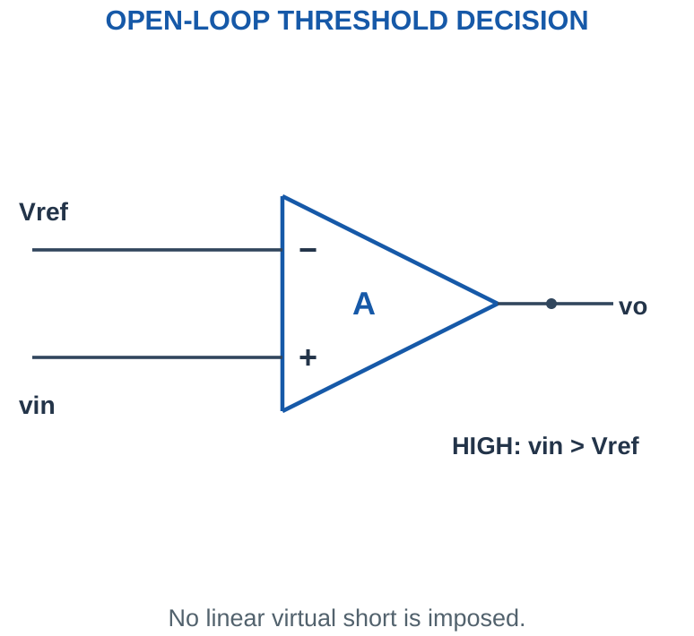
Decision rather than proportional amplification: A comparator normally operates in its limiting states. No negative feedback forces the two inputs equal, so never impose a virtual short. Reversing the input connections reverses the decision. At exact equality, offset and noise make a practical output uncertain.
An op-amp demonstrates the principle, but a dedicated comparator is usually selected for reliable switching speed and logic interfacing. Op-amps can recover slowly from saturation, may have restricted differential inputs and may deliver output voltages incompatible with a digital input. Verify those details before treating a triangle as a universal logic device.
One-line rule: Write “HIGH if v+ > v-” before substituting values. It works for either input arrangement and avoids memorising two unrelated rules.
Worked Problem 3.16: Comparator State and Output Level
Problem: v+ = 3 V and v- = 2.5 V. Specified HIGH = 10 V and LOW = -10 V. Find the ideal decision; practical input ranges are assumed compatible.
Model / approach: Compare the imposed inputs without applying a virtual short.
Step 1: vd = v+ – v- = 0.5 V.
Step 2: The decision is HIGH; output level is 10 V.
Answer: HIGH; vo = 10 V.
Check and interpretation: Use the supplied output levels. They are not automatically equal to the rails, and a logic input connected afterward would need a separate voltage-compatibility check.
20. Threshold Dividers and Zero Crossing
A reference divider creates Vref = VS Rbottom/(Rtop + Rbottom) when its loading is negligible. The ratio, not the total resistance alone, sets the ideal threshold. Real input bias current and other connected loads can alter it.
A zero-crossing detector uses a threshold at the defined zero reference. With a bipolar input and compatible supplies, the output changes state as the input crosses zero. A single-supply implementation may instead compare a biased signal with a mid-supply reference; crossing that reference represents the signal’s local zero.
For an input vin = VDC + Vp sin(ωt), the threshold must lie within VDC ± Vp for crossings to occur. A threshold at an extreme gives only a touching event in the ideal mathematical waveform, not a robust pulse. Real noise near a slowly crossed threshold can cause repeated transitions.
Divider trick: To obtain a fraction a of VS, choose Rbottom/Rtop = a/(1 – a). Confirm the fraction lies strictly between zero and one for a passive two-resistor divider.
Worked Problem 3.17: Divider Threshold
Problem: A negligible-load divider uses VS = 5 V, Rtop = 30000 Ω and Rbottom = 20000 Ω. A sensor enters comparator + and the divider enters -. Find the threshold and state at a sensor voltage 0.2 V above it.
Model / approach: Find the divider voltage, then apply v+ > v-.
Step 1: Vref = 5 × 20000/(30000 + 20000) = 2 V.
Step 2: At sensor voltage 2.2 V, v+ exceeds v- by 0.2 V, so the output is HIGH.
Answer: Threshold = 2 V; tested state = HIGH.
Check and interpretation: The actual HIGH voltage is not given and should not be invented. The negligible-loading assumption excludes input-bias and other divider-loading errors.
21. Noise, Hysteresis and Decision Margins
If a noisy sensor drifts slowly around a single threshold, the output may chatter. Hysteresis introduces two switching thresholds: one for a rising input and another for a falling input. The separation creates a dead band that prevents small reversals from immediately undoing the decision.
Worked check: Decision margin at a noisy boundary
For a single threshold 2.5 V, a nominal sensor voltage 2.52 V with possible ±0.05 V noise can fall as low as 2.47 V. It can cross the threshold despite being nominally above it. A decision margin must account for the actual uncertainty and the chosen input polarity.
Worked check: Hysteresis width versus state
With rising threshold 3 V and falling threshold 2 V, the width is 1 V. An input fixed at 2.4 V can correspond to either output state depending on history. The width alone does not determine that state; identify the last crossing or state an initial condition.
COMPARATOR DECISION
| Input Relation | Output Tendency |
|---|---|
| v+ > v- | Toward the stated HIGH level |
| v+ < v- | Toward the stated LOW level |
| Inside hysteresis band | Use previous state and crossing history |
An output level is not automatically the supply voltage. Check compatibility with the next interface.
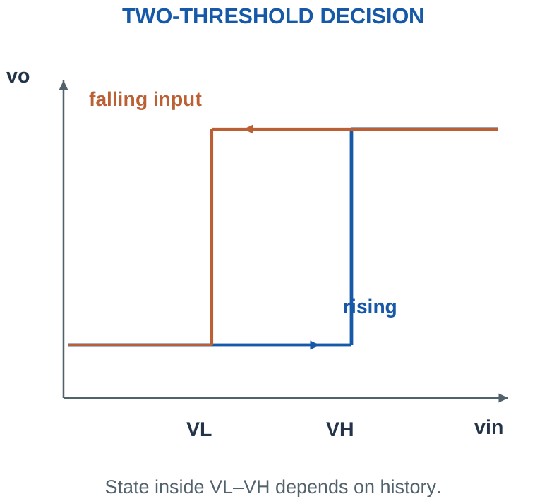
Introductory state calculation: When thresholds are supplied, compare the input with the appropriate threshold for the present state. For a non-inverting hysteretic decision that turns HIGH on a rise through VH, use VL to return LOW during a fall. Inside VL < vin < VH, retain the previous state. Without an initial state or previous crossing, the output is not uniquely specified.
This is an application extension, not the ordinary linear negative-feedback gain calculation. Positive feedback intentionally reinforces a decision, so v+ = v- is not a general operating rule. A real design also needs compatible output levels and a valid resistor-network calculation.
Exam distinction: Noise amplitude smaller than the hysteresis width is not alone a universal guarantee of no switching. The operating point and distance to the active threshold also matter.
Worked Problem 3.18: Follow the Threshold History
Problem: A non-inverting hysteretic decision switches HIGH above 3 V and LOW below 2 V. Initially LOW. Apply inputs 1, 2.5, 3.2, 2.5, 1.8 V in that order. Find the states.
Model / approach: Use the active threshold and retain state inside the 2–3 V band.
Step 1: 1 V: LOW. Rising to 2.5 V: still LOW because 3 V was not exceeded.
Step 2: 3.2 V: HIGH. Falling to 2.5 V: stays HIGH until the input goes below 2 V.
Step 3: 1.8 V: LOW. Hysteresis width = 3 – 2 = 1 V.
Answer: LOW, LOW, HIGH, HIGH, LOW.
Check and interpretation: The same 2.5 V input has different states depending on the preceding crossing. A single input value inside the band without history is insufficient to predict the output.
22. Temperature-Sensor Amplification
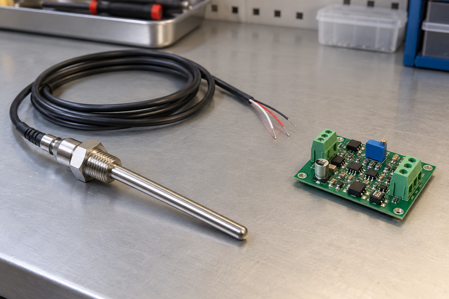
A temperature sensor converts temperature into a voltage or another electrical quantity. For a stated linear voltage model vS = S T + b, S is sensitivity and b is the zero-temperature intercept. The conditioning stage scales and, when needed, shifts this voltage for the next circuit.
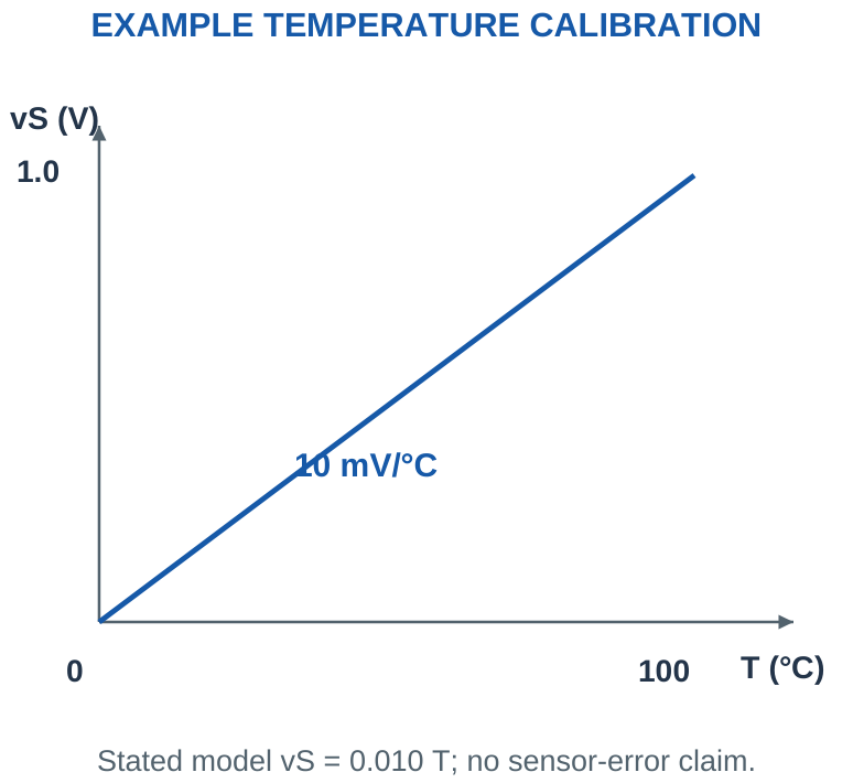
Design from endpoints: Write both input endpoints and both desired output endpoints. For vo = a vS + c, a = (vo,max – vo,min)/(vS,max – vS,min), then c = vo,min – a vS,min. Choose an amplifier topology that can implement both slope and intercept. A plain grounded non-inverting stage only multiplies; it does not independently subtract an unwanted sensor offset.
Check the op-amp input range, output swing and load. The sensor’s physical temperature range and self-heating are separate considerations from the algebraic gain. Never claim accuracy from a nominal sensitivity alone; sensor error, reference error, resistor tolerance and op-amp offset all contribute.
Quick check: If a 10 mV/°C model is amplified by 5, the output slope is 50 mV/°C. A voltage offset at the output corresponds to a temperature error equal to that offset divided by this slope.
Worked Problem 3.19: Temperature Scale and Amplified Sensitivity
Problem: A stated sensor model is vS = 10 mV/°C × T over 0–100 °C. An ideal non-inverting stage has gain 4. Find full-scale output and output sensitivity. Assume a suitable device and output range.
Model / approach: Scale both voltage endpoints and the calibration slope.
Step 1: At 0 °C, vS = 0 V. At 100 °C, vS = 1 V.
Step 2: Full-scale output = 4 × 1 = 4 V.
Step 3: Output sensitivity = 4 × 10 = 40 mV/°C.
Answer: Output range 0–4 V; sensitivity 40 mV/°C.
Check and interpretation: These are nominal results for the supplied linear model, not a guarantee of sensor accuracy. A real amplifier must support input near zero and the output endpoints if those values are required.
23. Light Sensors and Divider Behaviour
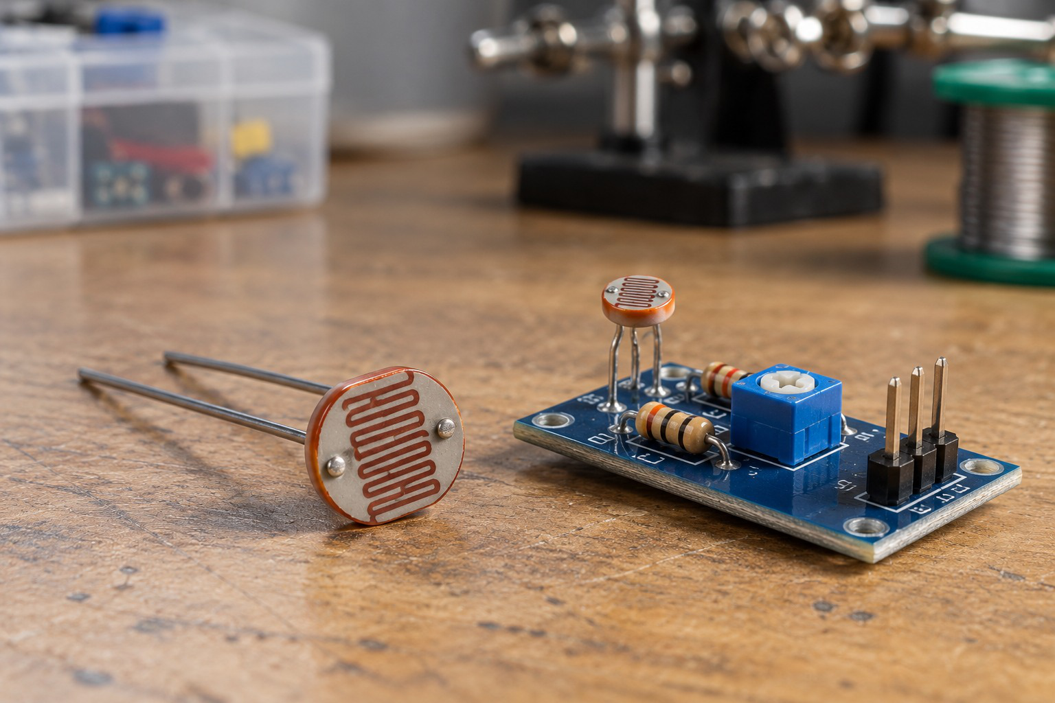
An LDR usually has lower resistance in bright light and higher resistance in darkness. Its resistance-versus-illumination characteristic is nonlinear and device dependent. A simple divider turns the resistance change into a voltage, after which an amplifier or comparator can process it.
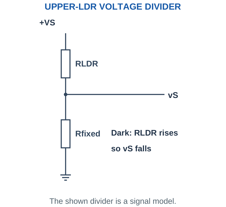
For the shown orientation, vS = VS Rfixed/(RLDR + Rfixed). As RLDR rises, the denominator rises and vS falls. Swapping the two divider elements reverses this trend. Always draw the orientation before deciding whether darkness produces a larger or smaller voltage.
A comparator can detect a light level without requiring linear conversion into lux. Accurate illumination measurement needs calibration and a suitable sensor; an arbitrary two-point LDR resistance example does not establish a universal lux scale.
Diagnostic trick: Test the limiting cases. Upper LDR approaching zero gives vS near VS; upper LDR becoming very large gives vS near zero. These endpoints reveal the correct direction immediately.
Worked Problem 3.20: Upper-LDR Divider Voltage
Problem: The upper divider element is RLDR = 1000 Ω from +5 V to the junction. The lower fixed resistor is 10000 Ω to ground. Find junction voltage.
Model / approach: The measured voltage is across the lower fixed resistor.
Step 1: vS = 5 × 10000/(1000 + 10000) = 4.5455 V.
Step 2: Divider current = 5/(1000 + 10000) = 454.5455 µA.
Answer: vS ≈ 4.5455 V.
Check and interpretation: Increasing the upper LDR resistance lowers this voltage. The supplied resistance is an educational light-condition value; it does not by itself specify illumination in lux.
24. Automatic Night Lamp Comparator Circuit
Use the upper-LDR divider from the preceding topic. Its voltage falls in darkness. Connect this sensor voltage to the – input and a stable threshold Vref to the + input. The output goes HIGH when vS < Vref, so the decision indicates darkness.
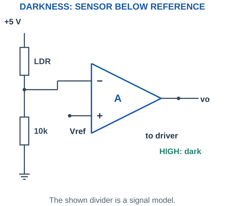
Decision and load path: The comparator output controls a compatible driver; it is not assumed to power a lamp directly. A transistor or another suitable interface handles load current. If the load is inductive, its switching arrangement needs the appropriate recirculation path. Keep the low-power decision circuit distinct from the load-power circuit.
At the nominal switching point, solve Vref = VS Rfixed/(RLDR + Rfixed), giving RLDR,th = Rfixed(VS/Vref – 1). This is a resistance threshold, not a calibrated illumination value. Hysteresis can reduce chatter near dusk; appropriate threshold values determine the turn-on and turn-off levels.
Implementation note: The illustrated 5 V divider describes a signal model with a compatible comparator. It is not a claim that a classic 741 can operate as a 0–5 V rail-to-rail device.
Worked Problem 3.21: Night-Lamp Resistance Threshold
Problem: Use a +5 V upper-LDR divider with lower Rfixed = 10000 Ω. Connect vS to – and Vref = 2.5 V to +. Find the threshold RLDR and states at 1 kΩ and 100 kΩ. Assume a compatible comparator and driver.
Model / approach: Darkness raises RLDR and lowers vS; HIGH indicates darkness.
Step 1: RLDR,th = 10000(5/2.5 – 1) = 10000 Ω.
Step 2: At 1 kΩ, vS ≈ 4.5455 V > Vref, so output is LOW.
Step 3: At 100 kΩ, vS ≈ 0.4545 V < Vref, so output is HIGH.
Answer: Threshold = 10000 Ω; bright LOW, dark HIGH.
Check and interpretation: The result is a resistance boundary, not a calibrated lux boundary. Equality is the transition condition; practical offset and noise make a small decision margin desirable.
25. Pressure-Sensor Conditioning
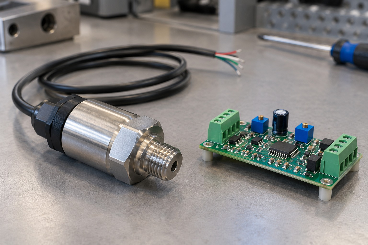
Pressure sensors may provide a small voltage difference, a bridge output or an already conditioned voltage. Read the stated sensor model before choosing a circuit. A simple sensitivity in mV/kPa must be combined with its intercept and allowed pressure interval.
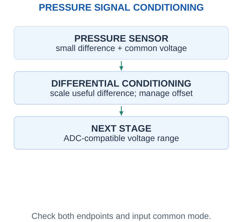
For a sensor vS = S P + b, the desired output is obtained by scaling and, if necessary, removing or adding an offset. A differential amplifier can subtract a reference before scaling. A high common-mode voltage can coexist with a tiny differential signal; both input pins must remain within their permitted common-mode range.
Bridge excitation accuracy can affect sensitivity, and resistor matching influences rejection of common-mode changes. Do not confuse “zero pressure output” with a ground connection. A sensor can have a nonzero output at zero pressure and still have a perfectly valid linear calibration model.
Endpoint check: A chosen gain that gives the correct full-scale voltage can still give the wrong zero-scale voltage. Verify both ends, then check an interior point.
Worked Problem 3.22: Pressure Calibration from Endpoints
Problem: The model vS = 0.5 V + (10 mV/kPa)P applies over 0–50 kPa. Map it to 1–5 V. Find slope a, intercept c and output at half-scale pressure.
Model / approach: Calculate the sensor span before determining the amplifier transfer.
Step 1: Sensor endpoints = 0.5 V and 1 V; span = 0.5 V.
Step 2: a = (5 – 1)/0.5 = 8; c = 1 – a × 0.5 = -3 V.
Step 3: At 25 kPa, vS = 0.75 V and vo = 3 V.
Answer: vo = 8vS + (-3 V); midpoint output = 3 V.
Check and interpretation: The algebra defines a desired conditioning transfer. It does not claim that an arbitrary single grounded non-inverting stage implements an independent offset term.
26. Op-Amp Audio Amplification
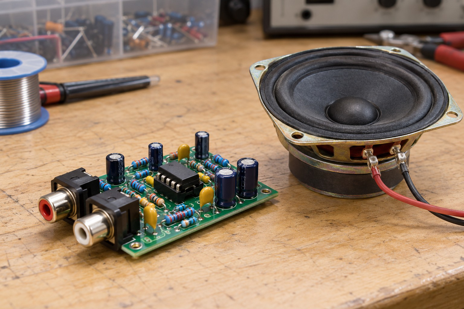
An audio voltage amplifier raises a small varying voltage for a later stage. An op-amp can provide useful voltage gain, but a general-purpose signal op-amp is not automatically a loudspeaker power amplifier. Load impedance, required current, dissipation, bandwidth and output swing matter.
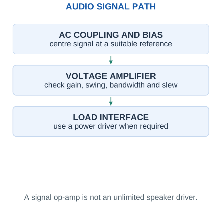
Amplitude and reference: On a dual supply, a small signal can swing around zero. On a single supply, an AC-coupled input is commonly biased around a suitable reference. The output then swings around its quiescent value. Its maximum peak amplitude is limited by the smaller distance to the upper or lower permitted output level.
For a sine wave, VRMS = Vpeak/√2 and Vpp = 2Vpeak. Voltage gain in decibels is 20 log10|Av|. Keep peak, peak-to-peak and RMS quantities consistent. Multiplying an RMS input by voltage gain produces an RMS output only while the amplifier remains linear and frequency response is appropriate.
Clipping check: For an output biased at 2.5 V with a permitted 0.5–4.5 V swing, the maximum zero-centred AC peak around that bias is 2 V, not 4 V.
Worked Problem 3.23: Audio RMS, Peak and Load Power
Problem: A sine input is 0.1 V RMS and voltage gain is 10. Load = 1000 Ω. Find output RMS, peak, peak-to-peak and ideal load power, assuming linear operation.
Model / approach: Gain multiplies RMS; convert the output amplitude consistently.
Step 1: Vo,RMS = 0.1 × 10 = 1 V.
Step 2: Vo,peak = √2 × 1 = 1.4142 V; Vpp = 2.8284 V.
Step 3: PL = VRMS²/RL = 1 mW.
Answer: 1 V RMS; 1.4142 V peak; 1 mW.
Check and interpretation: The assumed load is stated; do not substitute an 8 Ω speaker without checking output current. Power follows from the actual load voltage only while the amplifier remains linear.
27. Frequency Response and Gain-Bandwidth
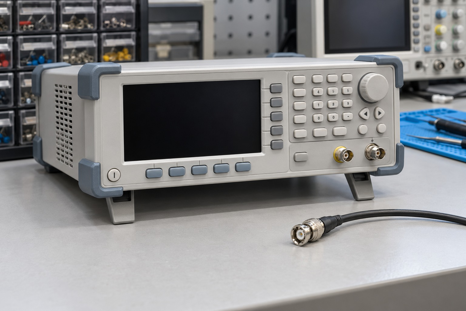
Closed-loop gain is approximately constant only over a finite frequency range. In a dominant-pole educational model, the gain-bandwidth product fT is approximately constant: closed-loop small-signal bandwidth fBW ≈ fT/NG, where NG is the noise gain.
Worked check: Unity inverter versus follower bandwidth
With a stated fT = 1 MHz, a follower has noise gain 1 and estimated bandwidth 1 MHz. A unity inverter has signal gain -1 but noise gain 2, giving about 500 kHz. Equal signal-gain magnitudes do not make their elementary bandwidth estimates identical.
For a non-inverting amplifier, NG = 1 + Rf/Rg. For an inverting amplifier, signal gain is -Rf/Rin while NG = 1 + Rf/Rin. Use the noise gain in the elementary bandwidth estimate. A gain of -1 therefore has noise gain 2, unlike a follower with noise gain 1.
The response magnitude of the assumed first-order model is |A(f)| = A0/√(1 + (f/fBW)²). Its phase also changes with frequency. This relation is an approximation, not a complete device stability analysis. A large output may encounter slew limitation before this small-signal bandwidth is reached.
Numerical convention: When a problem gives fT = 1 MHz, treat it as the stated model value. It is not a guaranteed bandwidth for every 741 grade and operating condition.
Worked Problem 3.24: Bandwidth Uses Noise Gain
Problem: A non-inverting stage has feedback/input resistance ratio 9. Use a stated dominant-pole fT = 1 MHz. Find signal gain, noise gain and estimated bandwidth.
Model / approach: For these circuits, NG = 1 + resistor ratio.
Step 1: Signal gain = 10; noise gain = 10.
Step 2: fBW ≈ fT/NG = 1000000/10 = 100 kHz.
Answer: Estimated small-signal bandwidth ≈ 100 kHz.
Check and interpretation: For an inverter, using the signal-gain magnitude gives the wrong elementary estimate. This single-pole result does not establish stability for every device or remove the separate large-signal slew limit.
28. Slew Rate and Full-Power Bandwidth
Slew rate is the largest output-voltage rate of change a device can produce under stated conditions. It is expressed in V/µs or V/s. A requested rapid transition becomes a finite-slope ramp when the amplifier cannot move faster.
For a sinusoidal output vo = Vp sin(2πft), maximum slope is 2πfVp. Avoiding slew-induced distortion requires 2πfVp ≤ SR. Thus fmax = SR/(2πVp), or Vp,max = SR/(2πf). Convert 0.5 V/µs into 500,000 V/s before using hertz.
For a large voltage change ΔV, the slew-only lower bound on transition time is |ΔV|/SR. Actual settling may take longer because small-signal response, recovery and the required final accuracy also matter. This lower bound is not a complete settling-time specification.
Peak reminder: Use the sine-wave peak in the slew equation. If the question gives RMS or peak-to-peak output, convert it first.
Worked Problem 3.25: Maximum Sine Frequency from Slew Rate
Problem: Given SR = 0.5 V/µs and required output peak = 5 V, find the maximum frequency allowed by the sine-wave slew criterion.
Model / approach: Use SR in V/s and peak amplitude, not RMS.
Step 1: SR = 500000 V/s.
Step 2: fmax = SR/(2πVp) = 500000/(2π × 5) ≈ 15.9155 kHz.
Answer: Slew-limited frequency ≤ 15.9155 kHz.
Check and interpretation: This is a necessary slope condition, not a guarantee of low distortion at the exact bound. Small-signal bandwidth, output current and voltage swing must also satisfy the application.
29. ECG and EEG Front-End Concept
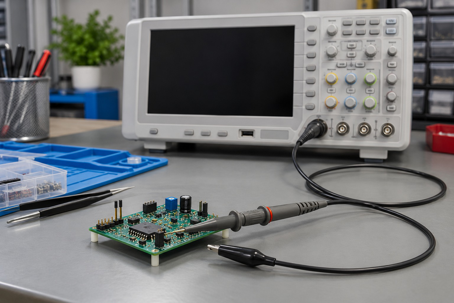
ECG and EEG are examples of small biological electrical signals measured as differences between sensing locations. The useful differential component may coexist with common-mode interference, electrode offsets and unwanted frequency components. The syllabus asks for the front-end concept, not a patient-connected construction circuit.
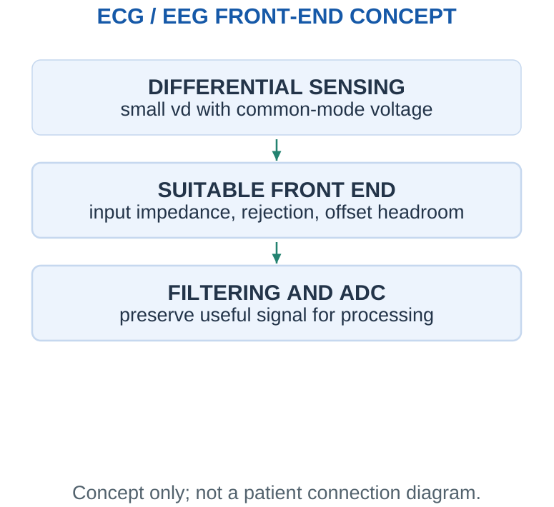
A suitable front end should load the source lightly, preserve the small difference, reject common-mode interference and accommodate electrode DC offsets without saturating. An instrumentation amplifier or a dedicated biopotential front end can provide functions a bare four-resistor subtractor does not automatically provide. Filtering limits unwanted low- and high-frequency content before further processing.
A 741 triangle is useful for explaining subtraction, but it is not a complete or appropriate medical front end by itself. Actual patient-connected systems require specialised protection and isolation design. For numerical learning, use stated differential signals and gains as abstract electrical inputs.
Key distinction: High CMRR reduces common-mode response within valid ranges. It does not remove differential interference, prevent every motion artefact or permit arbitrary electrode offsets.
30. Differential Gain Allocation and Headroom
Applying all desired gain in the first stage can amplify a large DC offset into saturation. A conceptual signal chain can first accommodate the offset, remove unwanted DC in a suitable filtering stage and then add gain. Every stage must be checked against its own input and output ranges.
If two cascaded voltage stages have gains G1 and G2, total gain is G1G2 under negligible loading and adequate bandwidth. Output offset and noise do not necessarily scale in the same way as the original desired signal because they may enter at different stages. Avoid describing the first stage’s tiny signal as already immune to later clipping.
In an ECG/EEG conceptual problem, first calculate the desired differential output. Then calculate any residual common-mode error from the supplied CMRR and the output due to a specified DC differential offset. These checks answer different questions and should not be collapsed into one “gain” result.
Headroom trick: An excellent small-signal gain can coexist with an unusable DC operating point. Calculate the baseline before adding the signal peaks.
31. Sensor Vocabulary, Calibration and Loading
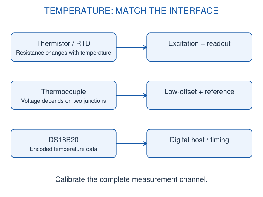
A sensor responds to a physical or chemical variable; a transducer converts energy or information between forms. A temperature element may change resistance, a thermocouple generates a small voltage, and a digital sensor includes conversion electronics. Choose the interface from the actual output type.
Signal conditioning includes excitation where required, buffering, amplification, offset adjustment, filtering and protection before conversion. Calibration establishes the relation between indication and a reference under stated conditions; it does not remove every source of drift.
Specifications: Range is the permitted input interval; sensitivity is the local output change per input change; resolution is the smallest indicated increment. Accuracy, repeatability and response time are different quantities. Loading can change the quantity being measured: a pH electrode needs a very high-input-impedance buffer.
Measurement workflow: Define the variable and range → choose the sensing principle → provide suitable excitation → condition the signal → calibrate → check uncertainty and response. A sensor symbol alone does not specify its power supply or its output scaling.
32. [B & C] Thermistors and Temperature Dividers
A thermistor is a strongly temperature-dependent resistor. An NTC type normally decreases in resistance as temperature rises; a PTC type has the opposite trend over its specified region. NTC elements offer high sensitivity over a limited interval but are nonlinear.
For a divider with fixed resistor RF at the top and thermistor RT to ground, Vnode = VS RT/(RF + RT). Heating an NTC lowers this node voltage. Interchanging the two elements reverses the trend. The amplifier must accept the full node-voltage range.
A local sensitivity ΔR/ΔT is useful only near its stated temperature. For a wider range use the supplied calibration table or a specified thermistor equation; do not extrapolate one local slope across the full range. Dissipation I²R causes self-heating and can bias the reading.
Conditioning: Use a stable excitation, buffer a high-resistance divider, filter noise to the required response speed, and calibrate the assembled sensor. A comparator converts a calibrated voltage threshold into a temperature alarm; it does not directly measure temperature.
Worked Problem 3.26: NTC Divider
Problem: A 5 V divider has RF = 10 kΩ above an NTC to ground. RT changes from 10 kΩ to 6 kΩ. Find both node voltages.
Model / approach: Use the lower-arm divider relation.
Step 1: Initially V = 5 × 10/(10 + 10) = 2.5 V.
Step 2: After heating V = 5 × 6/(10 + 6) = 1.875 V.
Answer: 2.50 V initially; 1.875 V after heating.
Check: The lower NTC resistance pulls the node toward ground.
Worked Problem 3.27: Local Thermistor Sensitivity
Problem: Near 25 °C, R = 10 kΩ and the supplied local slope is -400 Ω/°C. Estimate R at 27 °C.
Model / approach: Local linear approximation only.
Step 1: ΔT = 2 °C.
Step 2: ΔR ≈ -400 × 2 = -800 Ω.
Answer: R ≈ 9.20 kΩ.
Check: Do not use this short-range approximation over a wide temperature span.
33. [B] PT100 Resistance Temperature Detector
A PT100 is a platinum resistance temperature detector with nominal resistance 100 Ω at 0 °C. Platinum gives a reproducible positive temperature coefficient. The simple model R(T) = R0(1 + αT), with α supplied in the problem, is a linear approximation rather than a universal exact calibration.
A small constant current converts resistance to voltage: V = IR. Amplify the change above the reference level instead of wasting the output range on the fixed 0 °C voltage. Keep excitation low enough to limit self-heating; verify the sensor assembly and its thermal contact.
Two-wire lead resistance adds to the reading. Three-wire compensation relies on matched lead resistance and the appropriate circuit; a four-wire measurement separates force-current and sense-voltage connections. Specify the wiring before claiming lead-error cancellation.
Application: Reactor temperature monitoring combines a properly installed PT100, excitation and differential measurement, calibration and a controller. Sensor range, chemical compatibility, lag and fault detection matter along with electrical gain.
Worked Problem 3.28: PT100 Resistance
Problem: Use R0 = 100 Ω and α = 0.00385/°C. Estimate resistance at 80 °C.
Model / approach: Specified linear model.
Step 1: αT = 0.308.
Step 2: R = 100(1 + 0.308).
Answer: 130.8 Ω.
Check: The positive temperature coefficient gives resistance above 100 Ω.
Worked Problem 3.29: RTD Voltage and Heating
Problem: A 120 Ω RTD carries 1 mA. Find sensed voltage and electrical power.
Model / approach: Ohm’s law and Joule heating.
Step 1: V = 0.001 × 120 = 0.120 V.
Step 2: P = (0.001)² × 120 = 0.000120 W.
Answer: 120 mV; 0.120 mW.
Check: Temperature rise additionally requires a thermal dissipation model.
34. [B & C] Thermocouples and Reference Junctions
A thermocouple uses two dissimilar conductors. Its thermoelectric voltage depends on the temperatures of the measuring and reference junctions. The small output is commonly expressed in microvolts per degree over a local calibrated interval.
With an explicitly supplied constant sensitivity S, E ≈ S(Thot – Tref). Real conversion is nonlinear and type dependent. Measuring E alone cannot determine Thot unless the reference-junction temperature is also known or compensated.
Cold-junction compensation measures the local terminal temperature and applies the equivalent correction using the correct thermocouple relation. It does not physically force the terminal to 0 °C. Use appropriate extension wiring and avoid unintended thermal junctions.
An amplifier must handle microvolt signals, offset, noise and common-mode conditions. Low-pass filtering improves rejection of unwanted variation but increases response time. In a hot process, place the probe correctly and select a suitable sheath and temperature range.
Worked Problem 3.30: Thermocouple Voltage
Problem: Assume S = 40 µV/°C, hot junction 150 °C and reference 25 °C. Find E.
Model / approach: Supplied constant-sensitivity model.
Step 1: ΔT = 150 – 25 = 125 °C.
Step 2: E = 40 × 125 = 5000 µV.
Answer: 5.00 mV.
Check: The temperature difference, not hot temperature alone, sets the voltage.
Worked Problem 3.31: Reference-Junction Correction
Problem: A thermocouple gives 3 mV with S = 40 µV/°C and reference temperature 30 °C. Find hot temperature.
Model / approach: Invert the stated local model.
Step 1: Thot – Tref = 3000/40 = 75 °C.
Step 2: Thot = 30 + 75.
Answer: 105 °C.
Check: Ignoring the reference would understate the hot temperature by 30 °C.
35. [C] DS18B20 Digital Temperature Sensing
The DS18B20 integrates a temperature sensor, conversion and a digital 1-Wire interface. A host initiates conversion and reads encoded data; this differs from directly amplifying an analog thermistor voltage. A pull-up and the documented timing are required on the data line.
At the 12-bit setting the temperature increment is 0.0625 °C per count. This is resolution, not a claim of ±0.0625 °C accuracy. Signed raw values must be interpreted using the documented representation; the positive examples below avoid encoding ambiguity.
Allow conversion time, check communication and verify the reported data. The presence of a digital output does not eliminate thermal lag, mounting error or supply problems. External-power and parasite-power arrangements have different requirements.
Application: A fermenter temperature channel may use a suitably packaged probe, digital acquisition and a calibrated threshold. Packaging and process compatibility must be established independently of the sensor IC specification.
Worked Problem 3.32: Digital Temperature Count
Problem: At 12-bit resolution a positive DS18B20 raw value is 400 counts. Use 0.0625 °C/count.
Model / approach: Apply the stated resolution.
Step 1: T = 400 × 0.0625.
Answer: 25.0 °C.
Check: Resolution does not equal absolute measurement accuracy.
36. [C] Capacitive Humidity Measurement
A capacitive humidity element changes dielectric behaviour as it exchanges moisture with its surroundings. The electronics convert the capacitance change into an analog or digital relative-humidity indication. Relative humidity depends on temperature as well as water-vapour content.
A stated linear output model V = V0 + k RH gives RH = (V – V0)/k. Use that relation only within the supplied calibrated range. Condensation, contamination, temperature gradients and equilibration time can invalidate a quick reading.
Conditioning: Use the specified excitation/readout circuit, temperature compensation where provided, and a filter compatible with the required response time. A comparator can indicate an excessive-humidity condition, while hysteresis prevents rapid toggling close to the boundary.
Worked Problem 3.33: Humidity Calibration
Problem: A calibrated sensor follows V = 0.8 + 0.03 RH, with RH in percent. The output is 2.3 V. Find RH.
Model / approach: Invert the supplied calibration.
Step 1: RH = (2.3 – 0.8)/0.03.
Answer: 50% RH.
Check: This assumes the stated temperature and valid calibration interval.
37. [B] Strain Gauges and Piezoresistive Pressure
A bonded resistance strain gauge changes resistance when its substrate stretches or contracts. The gauge factor is GF = (ΔR/R)/ε, where strain ε is dimensionless. Microstrain means 10^-6 strain. A gauge must be bonded and oriented to sense the intended deformation.
A piezoresistive pressure transducer converts diaphragm strain into resistance change. A bridge often produces a small differential voltage; the result may need an instrumentation amplifier, offset removal and temperature compensation.
Sensitivity stated in mV/V requires multiplication by excitation voltage. A sensitivity in mV/bar already describes an output-per-pressure relation under stated conditions. Do not mix the two unit conventions.
Process pressure: Establish gauge, absolute or differential reference, compatible wetted materials and the calibrated range. Provide suitable excitation and verify both input common-mode voltage and differential signal before choosing amplifier gain.
Worked Problem 3.34: Strain-Gauge Change
Problem: A 350 Ω gauge with GF = 2 experiences +500 microstrain. Find ΔR.
Model / approach: GF = (ΔR/R)/ε.
Step 1: ε = 500 × 10^-6 = 0.0005.
Step 2: ΔR = 350 × 2 × 0.0005.
Answer: +0.350 Ω.
Check: The fractional resistance change is 0.001, or 0.1%.
Worked Problem 3.35: Pressure Transducer Scaling
Problem: A calibrated transducer has zero output at 0 bar and sensitivity 2 mV/bar. Output is 12 mV. Find pressure and gain for 1.2 V.
Model / approach: Use the supplied voltage sensitivity.
Step 1: p = 12/2 = 6 bar.
Step 2: G = 1.2/0.012 = 100.
Answer: 6 bar; voltage gain 100.
Check: The sensitivity is mV/bar, not mV/V/bar.
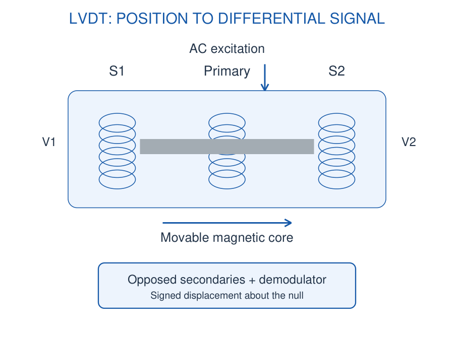
38. [B] LVDT Displacement Sensing
A linear variable differential transformer has one AC-excited primary, two secondary windings connected in opposition and a movable magnetic core. Core position changes the coupling to each secondary.
At the central null, the secondary voltages ideally cancel. Moving the core increases one coupling and decreases the other. The differential amplitude indicates displacement magnitude, while phase relative to excitation distinguishes direction.
Readout: AC excitation → differential secondary signal → phase-sensitive demodulation → low-pass filtering → calibrated displacement output. A raw unsigned AC amplitude alone cannot distinguish the two sides of null.
For a specified signed demodulated output Vout = kx in the linear range, x = Vout/k. LVDT sensitivity, permitted stroke, excitation frequency and loading are assembly-specific. The core should move freely without imposing an unintended mechanical force.
Worked Problem 3.36: LVDT Signed Difference
Problem: A demodulated LVDT channel defines Vout = V2 – V1. V2 = 1.8 V and V1 = 1.2 V. Find output and direction sign.
Model / approach: Preserve the declared polarity.
Step 1: Vout = 1.8 – 1.2.
Answer: +0.60 V; positive calibrated direction.
Check: Reversing the subtraction reverses the indicated direction.
Worked Problem 3.37: LVDT Displacement
Problem: A calibrated LVDT gives 0.25 V/mm in its linear range. Signed output is -0.75 V. Find displacement.
Model / approach: x = Vout/k.
Step 1: x = -0.75/0.25.
Answer: -3.0 mm from null.
Check: The negative sign gives direction; confirm 3 mm is within the stated stroke.
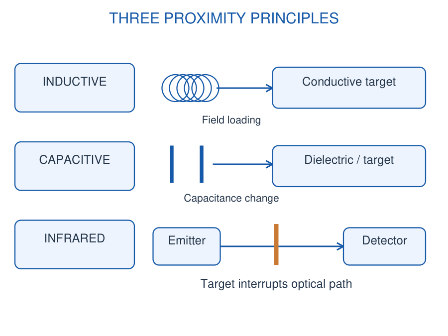
39. [B] Inductive, Capacitive and IR Proximity
Inductive: A driven coil produces an alternating field. A nearby conductive target changes the oscillator/loading through induced currents. It is useful for metal detection; range depends on target material, size and mounting.
Capacitive: An approaching target changes capacitance through geometry or dielectric properties. It can detect suitable nonmetallic materials as well as metals. The ideal parallel-plate relation C = εA/d explains trends, while a practical fringing-field sensor needs calibration.
Infrared: An emitter sends light and a detector receives transmitted or reflected energy. In a through-beam arrangement the target interrupts the path; in a reflective arrangement it changes returned light. Surface colour, alignment, ambient light and contamination affect operation.
Textile loom: Place an appropriate proximity sensor at the moving-part or yarn-monitoring position, condition its output and feed a controller input. Choose the sensing principle for the target: a metal-motion detector and an optical yarn detector are different applications.
Worked Problem 3.38: Capacitive Gap Change
Problem: An ideal air-gap capacitor has fixed area and capacitance 20 pF at 2 mm spacing. Find C at 1 mm.
Model / approach: C is inversely proportional to d for the ideal plate model.
Step 1: C2/C1 = d1/d2 = 2/1.
Answer: 40 pF.
Check: A real proximity sensor uses fringing fields and requires calibration.
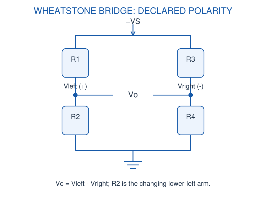
40. [B & C] Wheatstone Bridge and Differential Readout
Four resistors form two supply dividers. Let R1/R2 be the upper/lower left arms and R3/R4 the upper/lower right arms, with supply VS at the top and ground at the bottom. Define Vo = Vleft – Vright. Then Vo = VS[R2/(R1 + R2) – R4/(R3 + R4)].
The bridge balances when R1/R2 = R3/R4. Equal initial arms give zero ideal output. A change in one arm creates a small differential signal even though both midpoint voltages remain near half the excitation.
For initially equal arms and a small increase ΔR in the lower-left arm, Vo ≈ VS ΔR/(4R). The sign reverses if a different arm or output polarity is chosen. Use the exact divider expression when the fractional change is not small.
A differential or instrumentation amplifier must accommodate midpoint common-mode voltage, input bias requirements, offset and noise. More gain cannot recover a signal already corrupted by loading or an out-of-range input.
Worked Problem 3.39: Exact Bridge Voltage
Problem: VS = 5 V; R1 = R3 = R4 = 100 Ω and R2 = 102 Ω. Define Vo = Vleft – Vright.
Model / approach: Evaluate both divider voltages.
Step 1: Vleft = 5 × 10²/202 = 2.524752 V.
Step 2: Vright = 5 × 100/200 = 2.500000 V.
Answer: Vo = +24.752 mV.
Check: Both input nodes remain close to 2.5 V common mode.
Worked Problem 3.40: Small-Change Bridge Approximation
Problem: Use the bridge in the preceding problem. Estimate output with ΔR = 2 Ω, R = 100 Ω and VS = 5 V.
Model / approach: Quarter-bridge approximation.
Step 1: Vo ≈ VS ΔR/(4R) = 5 × 2/400 = 0.025 V.
Step 2: Difference from exact = 25.000 – 24.752 = 0.248 mV.
Answer: 25.0 mV; about 1.00% above the exact result.
Check: The approximation improves when ΔR/R becomes smaller.
41. [B] Industrial 4–20 mA and 0–10 V Signals
A 4–20 mA transmitter maps the lower range value to 4 mA and the upper value to 20 mA. The 4 mA live zero distinguishes a valid zero-scale measurement from some open-circuit faults; fault signalling details depend on the equipment.
For a linear calibrated range L to U, x = L + (I – 4 mA)(U – L)/(16 mA). A receiver resistor converts current to voltage, V = IR. With 250 Ω the nominal interval becomes 1–5 V; check resistor power and the receiver input range.
Why industrial current signalling? The receiver measures loop current, so series cable resistance does not directly form a signal-voltage divider while the transmitter remains within compliance. A broken wire can drive current below the valid minimum. Wiring resistance still consumes voltage and must be checked.
The loop supply must cover the transmitter minimum operating voltage, receiver drop, cable drop and any other series burdens. Current signalling tolerates cable resistance only while sufficient compliance voltage remains available.
Interface selection: Compare cable length, electrical interference, input impedance, isolation and fault detection. A current loop is not inherently noise-free, and a voltage input is not inherently inaccurate. The complete transmitter, wiring and receiver determine the result.
A 0–10 V output maps the range into voltage: x = L + (V/10 V)(U – L). Voltage signalling is simple but reference offsets, cable drops and loading can matter. Specify signal return, shielding and interface ratings. A 0 V reading can represent a valid lower-range value.
Worked Problem 3.41: 4–20 mA Process Reading
Problem: A 4–20 mA transmitter covers 0–100 bar. Current is 12 mA. Find pressure.
Model / approach: Remove live-zero current before scaling.
Step 1: Fraction = (12 – 4)/16 = 0.5.
Step 2: p = 0 + 0.5 × 100.
Answer: 50 bar.
Check: 12/20 is not the correct range fraction.
Worked Problem 3.42: Loop Receiver and Headroom
Problem: A 24 V loop has a transmitter needing at least 12 V, a 250 Ω receiver and 100 Ω total cable resistance. Check operation at 20 mA.
Model / approach: Add all series voltage burdens.
Step 1: Receiver drop = 0.020 × 250 = 5 V.
Step 2: Cable drop = 0.020 × 100 = 2 V.
Step 3: Available transmitter voltage = 24 – 5 – 2 = 17 V.
Answer: 1–5 V receiver range; 5 V headroom above the transmitter minimum at 20 mA.
Check: Receiver maximum dissipation is 0.020² × 250 = 0.10 W; choose a suitably rated resistor.
Worked Problem 3.43: 0–10 V Process Range
Problem: A 0–10 V channel represents 20–120 °C. Reading is 7.5 V. Find temperature.
Model / approach: Apply offset and span.
Step 1: Range fraction = 7.5/10 = 0.75.
Step 2: T = 20 + 0.75 × (120 – 20).
Answer: 95 °C.
Check: Zero volts represents 20 °C, not necessarily zero temperature.
42. [C] pH Electrode and Dissolved Oxygen
A biosensor combines a biological recognition element with a transducer. An enzyme-based electrode is one example. A sensor used in biotechnology is not automatically a biosensor: an ordinary temperature probe has no biological recognition element.
A glass pH electrode produces a high-source-impedance voltage relative to a reference electrode. At a stated temperature, an idealised local model is E = -S(pH – 7), with the polarity and zero explicitly defined. Sensitivity varies with absolute temperature; the supplied S must be used consistently.
Use a very high-input-impedance, low-bias-current buffer. A bias current IB through source resistance RS produces an approximate error IB RS; a large RS makes even a small current important. Buffer calibration, reference condition and contamination affect the reading.
Dissolved-oxygen sensors estimate oxygen concentration in a liquid using an appropriate electrochemical or optical principle. Output and compensation depend on the sensor. Temperature, pressure, salinity and flow can affect interpretation; do not equate an arbitrary voltage directly with oxygen concentration.
Two-point calibration: If specified reference outputs correspond to known concentration endpoints, interpolate within that range. An amplifier and filter can condition the electrical signal, but calibration establishes its chemical meaning.
Fermenter: Monitor temperature, pH and dissolved oxygen through separate calibrated channels. The controller compares measurements with set points and commands actuators through suitable interfaces. Probe sterilisation and process compatibility are part of the measurement design.
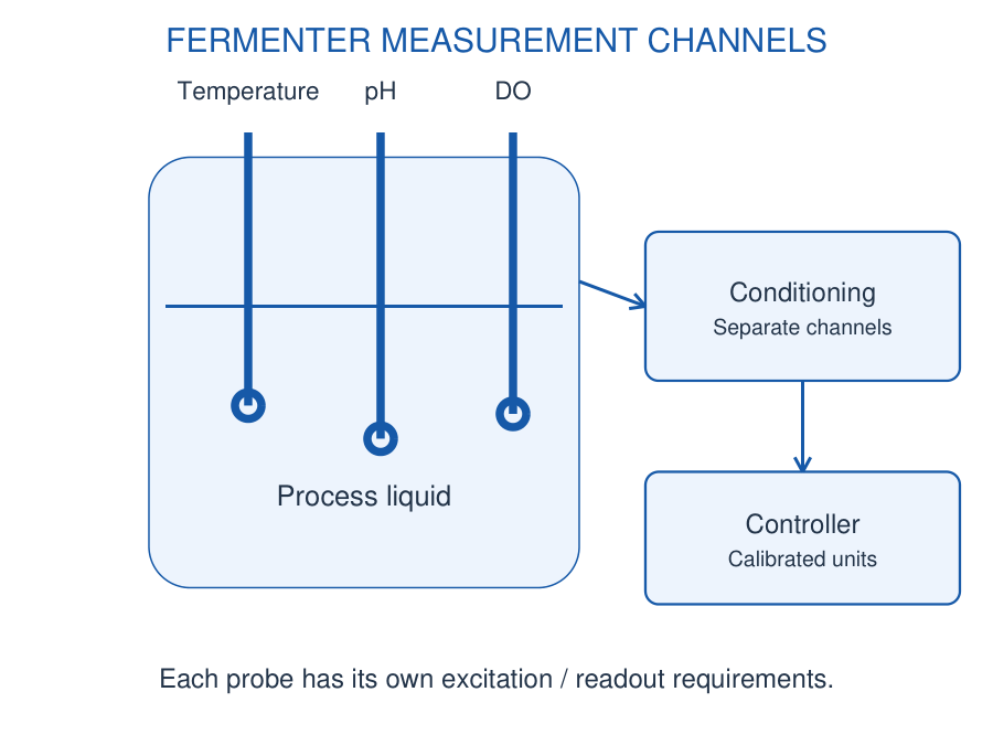
Worked Problem 3.44: pH Electrode Polarity
Problem: Use E = -0.05916(pH – 7) volts at the stated temperature. E = -0.11832 V. Find pH.
Model / approach: Keep the minus sign in the calibration.
Step 1: pH – 7 = -E/0.05916 = 2.
Answer: pH = 9.00.
Check: Changing the electrode polarity changes the voltage sign convention.
Worked Problem 3.45: pH Buffer Loading Error
Problem: Input bias current magnitude is 10 pA and electrode source resistance is 100 MΩ. Estimate voltage-error magnitude and equivalent pH error using 59.16 mV/pH.
Model / approach: IB RS loading-error model.
Step 1: Verror = 10 × 10^-12 × 100 × 10^6 = 0.001 V.
Step 2: pH error magnitude = 1/59.16.
Answer: 1.0 mV; approximately 0.0169 pH.
Check: Actual error polarity depends on bias-current direction and circuit arrangement.
Worked Problem 3.46: Dissolved-Oxygen Calibration
Problem: A calibrated DO channel gives 0.2 V at 0 mg/L and 2.0 V at 8 mg/L. Find concentration at 1.1 V.
Model / approach: Linear interpolation within the stated calibration.
Step 1: Fraction = (1.1 – 0.2)/(2.0 – 0.2) = 0.5.
Step 2: DO = 0.5 × 8.
Answer: 4.0 mg/L.
Check: Compensation and sensor condition must match the calibration assumptions.
43. [C] Soil Moisture, Light and NPK Measurement
A resistive soil-moisture probe infers wetness from conduction between electrodes. Salinity, soil composition and electrode corrosion can change the reading. A capacitive probe senses dielectric changes and can reduce exposed-electrode corrosion, but still needs soil-specific calibration.
A dry/wet normalisation such as index = (reading – dry)/(wet – dry) gives an instrument index under the stated conditions. It is not automatically volumetric water content. Check endpoint ordering: some circuits give a lower output when wetter.
An LDR changes resistance with illumination; a photodiode produces a light-dependent current. The readout may use a divider or a current-to-voltage stage. Optical geometry and spectral response matter, and a simple threshold gives an alarm rather than a universal lux reading.
NPK: Nitrogen, phosphorus and potassium assessment requires a validated nutrient-specific method or calibrated instrument. Electrical conductivity alone does not separately determine all three nutrient concentrations. Use the manufacturer-defined register/scaling or a supplied validated calibration, and report units clearly.
Photodiode conditioning: A transimpedance amplifier converts sensor current to voltage through a feedback resistor. Under the stated ideal polarity, vo = -Iphoto Rf relative to its reference. Choose resistance and compensation for the current range, capacitance and bandwidth; a larger resistor increases sensitivity but can reduce usable speed and headroom.
An agricultural monitoring chain is probe → validated readout → calibration/compensation → decision → actuator interface. Sensor supply energy and the information path are separate. Test sensor faults before allowing automatic irrigation or dosing.
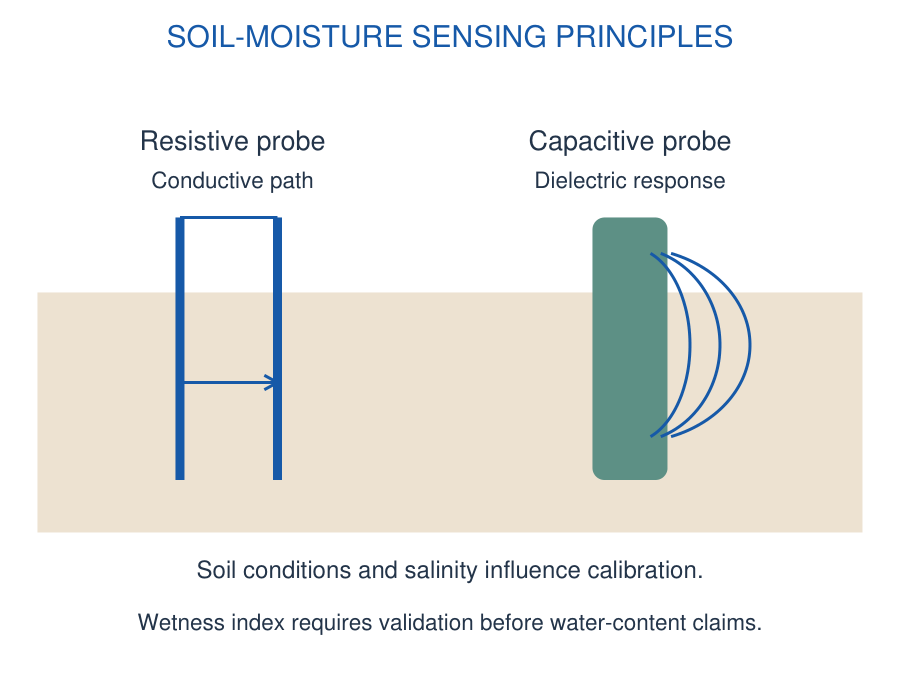
Worked Problem 3.47: Soil Wetness Index
Problem: Dry calibration reads 3.0 V and wet calibration 1.0 V. A reading is 1.8 V. Define index = (V – Vdry)/(Vwet – Vdry).
Model / approach: Normalise using both ordered endpoints.
Step 1: Index = (1.8 – 3.0)/(1.0 – 3.0) = 0.6.
Answer: 0.60, or 60% of this calibrated wetness-index span.
Check: This is not automatically 60% volumetric water content.
Worked Problem 3.48: Validated Nutrient Scaling
Problem: A validated instrument defines a nitrogen channel as 0.5 V at 0 mg/kg and 2.5 V at 100 mg/kg. Find the value at 1.3 V.
Model / approach: Use the supplied nutrient-specific calibration.
Step 1: Fraction = (1.3 – 0.5)/(2.5 – 0.5) = 0.4.
Step 2: Concentration = 0.4 × 100.
Answer: 40 mg/kg for this calibrated nitrogen channel.
Check: This relation does not claim that raw soil conductivity determines N, P and K separately.
44. [C] ECG and EMG Front-End Concepts
ECG and EMG are small biopotential signals acquired through electrodes. A differential front end amplifies the wanted difference while rejecting common-mode interference. High input impedance limits loading, but electrode imbalance and motion can still create artefacts.
Large gain should not be assigned blindly to the first stage: electrode offsets or interference may saturate it before filtering. Split gain across stages, check input common-mode range and output headroom, and choose bandwidth for the intended signal.
High-pass conditioning can remove slow baseline components; low-pass filtering limits high-frequency noise and supports anti-aliasing before sampling. A notch may suppress a narrow interference component, but filtering can also distort signal shape.
Study boundary: These are functional measurement concepts, not a patient-connected construction guide. Suitable protection, isolation, leakage control and complete medical-system design are separate requirements. An op-amp or filter alone does not establish patient safety.
Worked Problem 3.49: Biopotential Gain Allocation
Problem: A 2 mV differential signal must become 1 V. Use first-stage gain 20. Find total and second-stage gains.
Model / approach: Gtotal = G1 G2.
Step 1: Gtotal = 1/0.002 = 500.
Step 2: G2 = 500/20 = 25.
Answer: Total gain 500; second-stage gain 25.
Check: Check electrode-offset amplification, common-mode limits and output swing before accepting the design.
45. [B] Industrial Application Chains
Reactor temperature: PT100 or thermocouple → excitation/reference compensation → low-offset conditioning → calibrated temperature → controller. A thermocouple needs reference-junction compensation; a PT100 needs resistance measurement. They cannot share an unmodified interface.
Process pressure: Diaphragm bridge → differential amplifier → scaling → 4–20 mA or 0–10 V transmitter → receiver. Check the pressure reference, excitation, span and overload capability. The receiver converts the signal using the declared process range.
Loom monitoring: Proximity/optical detection → comparator with adequate noise margin → controller input → stop or indication command. Mechanical position, response time and target behaviour determine the sensor choice.
Civil structural tilt: A calibrated tilt transducer produces a signal related to inclination, conditioned and compared with baseline readings. Distinguish real structural movement from sensor mounting drift, thermal effects and vibration. A displacement LVDT measures tilt only through a defined mechanical geometry.
46. [C] Biotech and Agriculture Application Chains
Fermenter temperature and pH: Acquire each probe with its appropriate interface, convert using its calibration, compare with set points and record trends. Temperature compensation is part of pH interpretation; averaging unrelated raw voltages is meaningless.
Soil nutrient monitoring: Use validated N, P and K channels or a specified calibrated instrument. Confirm sampling depth, units and soil conditions. A threshold should be derived from the stated measurement objective, not copied from an arbitrary analog-to-digital count.
ECG front end: Electrodes → differential input stage → suitable filtering/gain → conversion/recording. Describe common-mode rejection, electrode offsets and headroom separately. Isolation belongs to the complete approved system architecture.
Memory cue: Sense the variable, preserve the signal, calibrate the units, then make the decision. More amplifier gain improves scale utilisation only when the signal, offset, noise and available output range remain compatible.
Worked Problem 3.50: Temperature Alarm Hysteresis
Problem: A sensor gives 10 mV/°C with zero offset. Alarm turns on at 60 °C and resets at 55 °C. Find thresholds and voltage hysteresis.
Model / approach: Convert both temperatures through the stated sensor relation.
Step 1: Von = 0.010 × 60 = 0.600 V.
Step 2: Vreset = 0.010 × 55 = 0.550 V.
Step 3: ΔV = 0.600 – 0.550 = 0.050 V.
Answer: 0.600 V ON, 0.550 V reset; 50 mV hysteresis.
Check: Comparator polarity and feedback network must implement the stated switching direction.
47. Circuit Analysis and Troubleshooting
Use a fixed sequence: identify topology; label inputs, output and rails; check feedback direction; write the appropriate equation; calculate the requested output; verify input range, output swing, current and speed. Only then interpret the answer as a valid linear result or a limiting state.
| Symptom | Useful First Check |
|---|---|
| Output at one limit | Missing feedback, reversed inputs, offset or excess gain |
| Wrong DC output | Wrong reference, ground path, offset or resistor value |
| Correct DC, bad fast signal | Bandwidth, slew rate or capacitive loading |
| Sensor voltage drops | Source resistance and input-network loading |
| Night lamp decision reversed | LDR orientation and +/- assignments |
| Difference circuit passes common signal | Resistor ratios and source resistance |
Do not diagnose every saturated output as a damaged device. A correct comparator is expected to reach a limiting level, while a linear amplifier at the same limit may have insufficient headroom. The intended operating mode determines whether the observation is normal.
48. Formula Sheet with Conditions
Three Conditions to Write in an Exam
Linear feedback: The equal-input approximation requires stable negative feedback and an achievable output.
Voltage ranges: The input common-mode range and output swing are distinct restrictions.
Model limits: Ideal formulas neglect specified nonideal effects unless the question introduces them.
Memory Cues
- Inverter: Ratio with minus.
- Non-inverter: One plus ratio.
- Summer: Add signed currents.
- Comparator: Compare plus with minus.
- Slew: Frequency times peak times 2π.
These cues are starting points; the connection diagram decides which one applies.
| Quantity | Expression and Conditions |
|---|---|
| Differential input | vd = v+ – v-; unsaturated vo = AOL vd |
| Inverting amplifier | Av = -Rf/Rin; ideal negative feedback |
| Non-inverting | Av = 1 + Rf/Rg; ideal negative feedback |
| Follower | Av ≈ 1; input/output ranges still apply |
| Inverting summer | vo = -Rf Σ(vi/Ri); virtual-ground conditions |
| Gain-bandwidth estimate | fBW ≈ GBW/noise gain; dominant-pole model |
| Sine-wave slew demand | SR ≥ 2πf Vpeak |
| Bridge | Vo = VS[R2/(R1 + R2) – R4/(R3 + R4)] |
| RTD linear estimate | R = R0(1 + αT); supplied interval |
| Thermocouple local model | E = S(Thot – Tref); stated sensitivity |
| 4–20 mA scaling | Fraction = (I – 4 mA)/(16 mA) |
| Calibration interpolation | x = L + (V – VL)(U – L)/(VU – VL) |
Model check: Verify feedback, signal polarity, common-mode range, output swing and bandwidth before applying a gain formula. Sensor calibration and amplifier gain are different operations.
CALIBRATION BEFORE DECISION
| Stage | Question |
|---|---|
| Sensor | What variable changes the output? |
| Conditioning | What gain, offset and filtering apply? |
| Calibration | What physical units correspond to the signal? |
| Threshold | What condition triggers and resets? |
Do not confuse digital counts, instrument index and physical concentration.
49. QUICK REVISION: EXPLAIN AND CHECK
When Is the Virtual Short Valid?
With stable negative feedback and linear unsaturated operation. It is an approximation, not a physical wire between inputs.
Why Can an Ideal-Gain Answer Fail?
The input common-mode range, output swing/current, bandwidth or slew rate may be exceeded.
Does a 741 Work from Any Supply?
No. It is not a rail-to-rail amplifier; consult its specified supply, load and signal ranges.
What Makes a Comparator Different?
It decides the sign of an input difference and drives toward an output limit; do not assume equal input voltages.
Why Add Hysteresis?
Separate rising and falling thresholds reduce repeated switching caused by noise near a threshold.
What Distinguishes RTD and Thermocouple?
The RTD changes resistance and needs excitation; a thermocouple gives a small voltage related to junction temperatures.
Why Compensate a Thermocouple Reference?
Voltage depends on both junction temperatures. A measured reference temperature permits the appropriate correction.
Is Digital Resolution Accuracy?
No. Count spacing and absolute measurement error describe different properties.
How Does an LVDT Show Direction?
The differential signal changes phase across null; signed demodulation preserves the direction.
Why Use a Bridge?
It converts resistance imbalance into a differential voltage, usually on a nonzero common-mode level.
Why Use 4 mA for the Lower Endpoint?
The live zero permits a valid minimum signal to be distinguished from some wiring faults.
Why Buffer a pH Electrode?
Its large source impedance makes loading and input bias current important.
Is a Soil Index Water Content?
Only if a valid soil-specific calibration establishes that relation. Endpoint normalisation alone gives an index.
Does Conductivity Measure All NPK Values?
No. Separate nutrient estimates require a validated nutrient-specific method or instrument.
Why Split ECG/EMG Gain?
Large electrode offsets can saturate an early high-gain stage. Allocate gain with offset, bandwidth and headroom checks.
What Is the Final Measurement Check?
Confirm units, calibration interval, excitation, loading, uncertainty and response time as well as the numerical answer.
| Task | Core Relation / Decision | Essential Check |
|---|---|---|
| Linear amplifier | Choose the correct feedback gain | Common-mode, swing, current and speed |
| Sensor readout | Apply excitation and calibration | Loading, temperature and stated range |
| Threshold alarm | Compare signal with reference | Polarity, hysteresis and interface levels |
| Biopotential front end | Differential gain plus filtering | Offsets, headroom and complete protection |