
Electronics Unit 2: Transistors, Switching and Amplification
Subject: Fundamentals of Electronics Engineering
University: AKTU
Course: B.Tech First Year
Semester: I & II
Course Codes: AEC101A / AEC201A | AEC101B / AEC201B | AEC101C / AEC201C
Applicable Streams: CSE, EE, ECE, CE, ME, CH, TX, BT & AG
Unit II Introduction
BJT construction, characteristics and load control lead into common-emitter amplification, MOSFET drive and switching. Optocouplers and dedicated industrial, biomedical and agriculture applications complete the combined unit.
Topics Covered
| Topic | Pages |
|---|---|
| BJT construction, currents and regions | 3–6 |
| Characteristics, bias and load line | 6–9 |
| BJT switches and inductive loads | 9–15 |
| CE amplification and class-A audio | 15–20 |
| FETs, MOSFET drive and PWM | 20–29 |
| Optocouplers and isolation | 29–31 |
| Industrial interfaces and SSRs | 31–33 |
| Biomedical and agri applications | 33–35 |
| Diagnosis, formulae and revision | 35–37 |
Coverage
All six A/B/C course codes and nine streams. The branch-wise topic guide identifies the relevant application sections. Read the shared foundation, then follow your prescribed application sections.
How to Use These Notes
- Identify switch, amplifier or isolation function first.
- Label B/C/E or G/D/S and mark voltage references.
- Trace control current separately from load energy.
- State the device model and verify its operating region.
- Try each problem before reading the worked answer.
- Check current capability, power and assumptions.
What Is Included?
| Study Support | Included |
|---|---|
| Worked problems | 50 numbered problems with steps and checks. |
| Labelled figures | Device structures, characteristics and circuit paths. |
| Realistic images | 10 component and application photographs. |
| Dedicated applications | Home automation, audio, industrial control, irrigation and biomedical systems. |
| Revision | Formula conditions, memory cues and short answers. |
Key Distinction
BJT saturation is an ON-switch state. The low-loss MOSFET ON model is normally the ohmic region. The same word does not mean the same operating condition in both devices.
Numerical Convention
Values are educational assumptions. Retain precision until the final answer. An approximate model is valid only within its stated conditions.
Unit Overview and Branch-Wise Reading Map
Read the shared switching foundation, then follow the topics prescribed for your branch group. A, B and C denote the course-code suffixes. Amplifier lessons are prescribed for A; the industrial and biomedical/agri application blocks are identified separately.
| Topics / Application Block | Applicable Branches | Where to Read |
|---|---|---|
| BJT construction, V-I characteristics, NPN, cut-off/saturation, relay drive | All nine streams | Sections 1–14 |
| FET introduction and MOSFET switch basics | All nine streams | Sections 21–29; advanced models are enrichment for B/C |
| PNP, active-region amplification, CE gain/bias, class-A audio | A: CSE, EE, ECE | Sections 3–5, 15–20 |
| MOSFET preference in digital ICs/power; home-automation relay and audio applications | A: CSE, EE, ECE | Sections 30–31 |
| PWM motor speed control | A: CSE, EE, ECE; B: CE, ME, CH, TX | Sections 28–29 |
| Optocoupler and isolation concept | B: CE, ME, CH, TX; C: BT, AG | Section 32 |
| Industrial relay, VFD gate drive, PLC output isolation and SSR | B: CE, ME, CH, TX | Sections 33–36 |
| Drip-irrigation valve, biomedical buzzer, solar-controller MOSFET and ECG isolation | C: BT, AG | Sections 37–40 |
| Diagnosis, formulae, solved problems and revision | All streams: select the relevant application | Throughout; Sections 41–43 |
Syllabus Groups and Official Unit Names
- A — CSE, EE, ECE: Transistors as Switches and Amplifiers.
- B — CE, ME, CH, TX: Transistors and Switching Circuits.
- C — BT, AG: Transistors and Simple Switching Circuits.
What Is Included
50 numbered worked problems with calculation steps and checks; 10 realistic component/laboratory images; labelled transistor circuits, characteristics and application illustrations. The two semester codes in each group use the same unit syllabus.
Study approach: Trace the current path, state the transistor model, calculate and verify the assumed state. A coloured [B] or [C] section label identifies additional group-specific coverage. Values in problems are stated educational assumptions.
1. THE TRANSISTOR: CONTROL AND ENERGY
A transistor controls current in one part of a circuit using an electrical condition applied at another terminal. In a switch, the intended output alternates between OFF and a low-loss ON state. In an amplifier, a small change around a suitable bias point produces a larger output change while the transistor remains in the intended operating region.
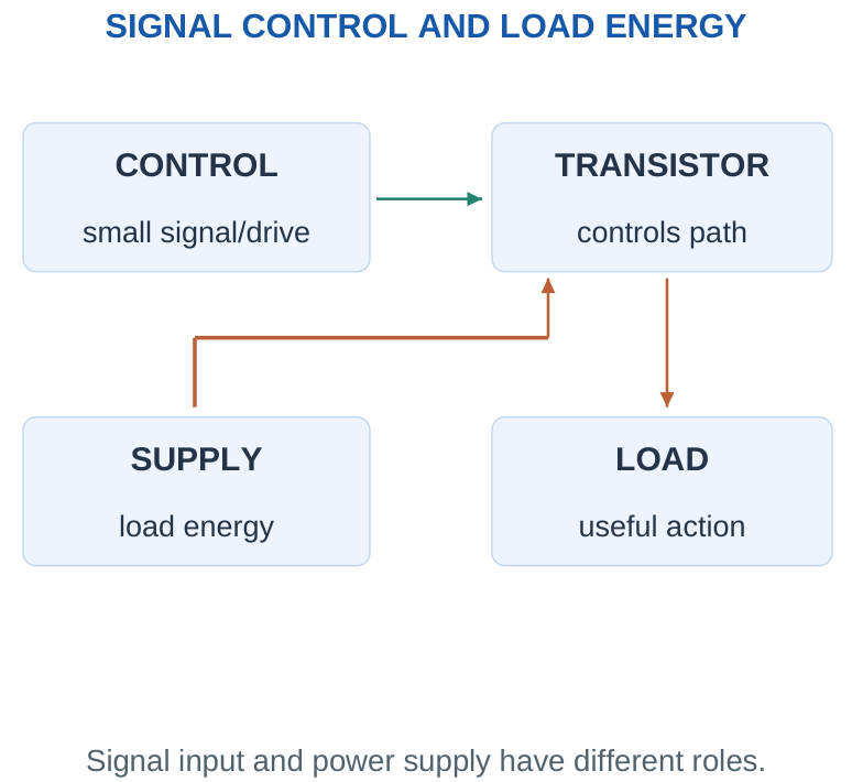
A BJT uses emitter, base and collector terminals. A MOSFET uses gate, source and drain, with a body terminal that is often internally connected to source in discrete power devices. Their control requirements and operating-region names are different. Do not transfer a BJT saturation rule unchanged to a MOSFET.
| Task | Desired Behaviour |
|---|---|
| Relay or indicator control | Clear OFF and adequately driven ON states. |
| Analog audio stage | Small changes about a stable operating point. |
| PWM motor stage | Repeated switching with controlled duty cycle. |
First question: Identify whether the transistor is being used as a switch or amplifier. That determines the region, model and performance checks needed before doing arithmetic.
2. BJT CONSTRUCTION AND CARRIER ACTION
A bipolar junction transistor has three semiconductor regions and two interacting junctions. An NPN device has a thin p-type base between n-type emitter and collector. A PNP has the complementary sequence. The emitter is designed for carrier injection, the base is thin and relatively lightly doped, and the collector is designed to collect carriers and withstand its intended electrical conditions.
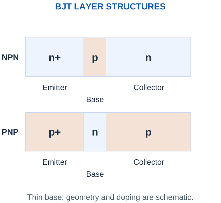
For an NPN in forward active operation, the base-emitter junction is forward biased and the base-collector junction is reverse biased. Electrons injected from the emitter cross the thin base; most are collected, while some recombination contributes to base current. Conventional collector current enters C and emitter current leaves E. PNP operation uses complementary carrier types and voltage/current polarities.
Two separate diodes connected back-to-back do not reproduce this controlled carrier transport through a common thin base. Similarly, reversing emitter and collector does not guarantee the original gain or voltage capability. Understand the physical arrangement before identifying a device only from a package shape.
Memory cue: Bipolar action involves electrons and holes. The emitter injects, the base controls the transport, and the collector collects; these words describe intended device roles rather than equal interchangeable terminals.
3. NPN, PNP AND CURRENT REFERENCES
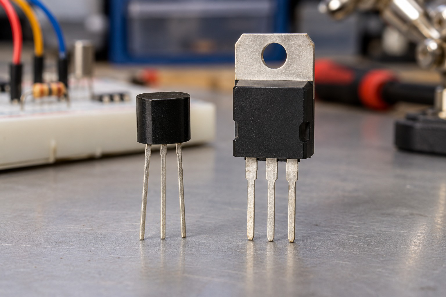
The BJT symbol’s arrow is on the emitter. For NPN it points outward; for PNP it points inward. Identify the arrow-bearing terminal before marking base and collector. A package pin order must come from the particular device information, not from assuming every three-lead transistor has the same arrangement.
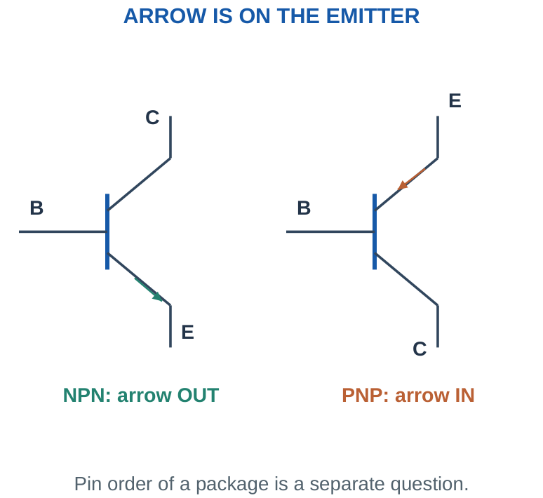
For an NPN using positive current magnitudes in its usual forward-active connection, IE = IC + IB. Define VBE = VB – VE and VCE = VC – VE. A PNP can be analysed with consistent signed quantities or with clearly stated positive magnitudes such as VEB = VE – VB. Mixing the two conventions inside one calculation causes false negative drops.
Worked check: Current-unit check
If IC = 8 mA and IB = 80 µA, convert 8 mA to 8,000 µA before dividing. β = 8,000/80 = 100. Emitter current is 8.08 mA. Keeping one current in milliamperes and the other in microamperes would create a factor-of-one-thousand error.
Memory trick: NPN: “Not Pointing iN.” PNP: arrow points in. This identifies the emitter arrow only; it does not replace checking the actual collector, base and emitter connections.
4. CURRENT GAIN: ALPHA AND BETA
In a stated forward-active model, β = IC/IB and α = IC/IE. Combining these definitions with IE = IC + IB gives α = β/(β + 1) and β = α/(1 – α). Alpha is close to, but below, one in the usual model; beta can be much larger than one.
The gain is not a fixed universal number for all devices, currents or temperatures. A supplied β is a calculation assumption for the stated operating condition. In saturation, a switch’s collector current is principally constrained by its load circuit and available drive, so blindly continuing IC = βIB can produce an impossible answer.
| Quantity | Meaning |
|---|---|
| β or hFE in a stated DC active model | Collector-current/base-current ratio. |
| α | Collector-current/emitter-current ratio. |
| Forced beta | Chosen or achieved IC/IB in a switch-drive calculation. |
Unit trick: Convert base microamperes and collector milliamperes to the same unit before dividing. For example, 5 mA/50 µA = 100, not 0.1.
Worked Problem 2.1: Terminal Currents and Gains
Problem: An NPN has IC = 5 mA and IB = 0.05 mA in a stated active condition. Find IE, β and α.
Model / approach: Use consistent positive magnitudes and IE = IC + IB.
Step 1: IE = 5 + 0.05 = 5.05 mA.
Step 2: β = 5/0.05 = 100.
Step 3: α = IC/IE = 5/5.05 ≈ 0.9901.
Answer: IE = 5.05 mA; β = 100; α ≈ 0.9901.
Check and interpretation: Alpha is below one because emitter current includes both collector and base currents. Gain definitions do not by themselves verify that an arbitrary external circuit can maintain this active operating point.
Worked Problem 2.2: Convert Beta to Alpha
Problem: For a stated active-region model, β = 49. Find α and the base-current fraction of emitter current.
Model / approach: Combine the gain definitions with KCL.
Step 1: α = β/(β + 1) = 49/50 = 0.98.
Step 2: IB/IE = 1/(β + 1) = 2%.
Answer: α = 0.98; base fraction = 2%.
Check and interpretation: The result concerns the supplied current model. It does not mean α and β remain exactly constant when device current, temperature or operating region changes.
5. CUT-OFF, ACTIVE AND SATURATION
For an NPN in forward active operation, BE is forward biased and BC reverse biased. In saturation, both junctions are forward biased. In cut-off, the device lacks the intended forward base drive and collector current is approximately zero in the introductory model, although real leakage can remain.
ASSUME → SOLVE → VERIFY
- Calculate the candidate base current.
- Use the stated active gain for a candidate IC.
- Apply collector-loop KVL.
- Check terminal voltages and junction biases.
A negative candidate VCE in the intended forward circuit rejects the active assumption; it is not the physical ON-switch answer.
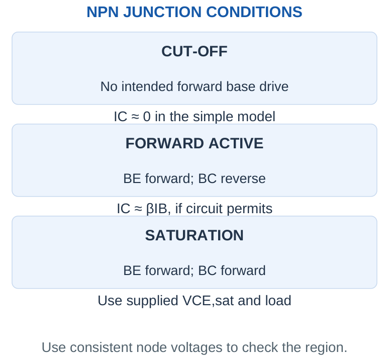
| Region | Introductory Purpose | Important Model |
|---|---|---|
| Cut-off | OFF switch. | IC approximately zero. |
| Forward active | Analog amplification. | IC approximately βIB, with region check. |
| Saturation | Adequately driven ON switch. | Small specified VCE,sat; load-limited current. |
A common switch exercise supplies VBE,on or VBE,sat and VCE,sat. Those are model values, not universal constants. For NPN active operation, checking VC > VB helps verify reverse-biased BC. If an active estimate predicts VC below VB, the assumed forward-active state is no longer consistent. Use the specified alternative model instead of reporting unlimited βIB.
Critical distinction: BJT saturation is commonly the desired low-voltage ON state for switching. MOSFET saturation names a different region and is generally not the low-RDS,on state sought for an efficient power switch.
Worked Problem 2.3: Use Terminal Differences
Problem: An NPN has VB = 0.7 V, VC = 5 V and VE = 0 V. Find VBE, VBC and VCE, and interpret the stated junction conditions.
Model / approach: Use VBE = VB – VE, VBC = VB – VC and VCE = VC – VE.
Step 1: VBE = 0.7 V; VBC = -4.3 V; VCE = 5 V.
Step 2: The positive BE condition and negative BC voltage are forward-active consistent under the introductory junction-bias interpretation.
Answer: Forward-active consistent; VCE = 5 V.
Check and interpretation: This interpretation assumes an ordinary forward-operated NPN and the stated voltage conditions. Current magnitudes still require the external circuit and a suitable device model; a positive supply value alone does not determine the region.
Worked Problem 2.4: Use Terminal Differences
Problem: An NPN has VB = 0.8 V, VC = 0.2 V and VE = 0 V. Find VBE, VBC and VCE, and interpret the stated junction conditions.
Model / approach: Use VBE = VB – VE, VBC = VB – VC and VCE = VC – VE.
Step 1: VBE = 0.8 V; VBC = 0.6 V; VCE = 0.2 V.
Step 2: The positive BE condition and positive BC voltage are saturation consistent under the introductory junction-bias interpretation.
Answer: Saturation consistent; VCE = 0.2 V.
Check and interpretation: This interpretation assumes an ordinary forward-operated NPN and the stated voltage conditions. Current magnitudes still require the external circuit and a suitable device model; a positive supply value alone does not determine the region.
6. COMMON-EMITTER INPUT CHARACTERISTIC

In the common-emitter configuration, input is applied between base and emitter and output is observed between collector and emitter. The input characteristic plots IB against VBE at a stated VCE. It resembles a forward junction curve over the usual conducting region, but its exact position depends on device and test conditions.
Worked check: Input voltage change
A local base-current increase of 5 µA requires a supplied 10 mV VBE change. The local input slope resistance is 0.010/(5 × 10^-6) = 2 kΩ. This change ratio belongs to that operating point and should not be substituted for the transistor’s complete nonlinear input behaviour.
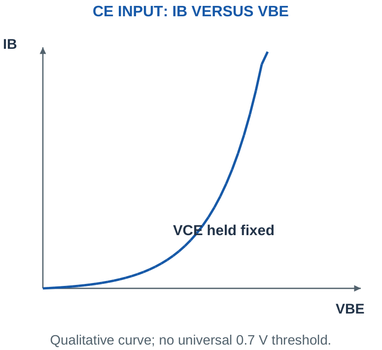
The local input resistance can be estimated from a supplied small change as rin ≈ ΔVBE/ΔIB around a specified operating point. This slope-based quantity differs from VBE/IB, a static ratio. Neither should be treated as a resistance that applies unchanged across cut-off, active and saturation regions.
A base resistor limits drive current from a voltage source. In a simple grounded-emitter input with a supplied VBE, IB = (Vdrive – VBE)/RB when the assumed junction conduction is valid. An input below the model’s conducting condition requires the OFF solution, not a negative forward base-current answer.
Graph habit: Write what is held constant next to a characteristic. Input means IB-VBE at fixed VCE; changing that to IC-VBE would be a different characteristic.
Worked Problem 2.5: Input Slope Versus Static Ratio
Problem: At a point, VBE = 0.70 V and IB = 20 µA. A nearby 10 µA increase requires a 15 mV increase in VBE. Find the static ratio and local input resistance.
Model / approach: Use a point ratio separately from a change ratio.
Step 1: VBE/IB = 0.70/(20 × 10^-6) = 35 kΩ.
Step 2: rin ≈ ΔVBE/ΔIB = 0.015/(10 × 10^-6) = 1.5 kΩ.
Answer: 35 kΩ static ratio; 1.5 kΩ local slope.
Check and interpretation: The two numbers describe different aspects of a nonlinear input characteristic. Neither is a fixed resistor that can be used unchanged across every transistor state.
Worked Problem 2.6: Base-Loop Current
Problem: A grounded-emitter NPN input uses Vdrive = 5 V, assumed VBE = 0.7 V and RB = 100000 Ω. Find base current under the conducting input model.
Model / approach: The base resistor sees Vdrive – VBE, not the complete drive voltage.
Step 1: VRB = 5 – 0.7 = 4.3 V.
Step 2: IB = VRB/RB = 43 µA.
Answer: IB ≈ 43 µA.
Check and interpretation: The positive current supports the assumed forward input state. Collector-region and driver-output checks remain separate. This calculation alone is not proof that a connected load will be saturated.
7. COMMON-EMITTER OUTPUT CHARACTERISTICS
The CE output characteristics plot IC against VCE for several fixed base currents. Near low VCE the curves enter the saturation region. In forward active operation, IC is relatively insensitive to VCE compared with its dependence on IB, although real curves need not be perfectly horizontal.
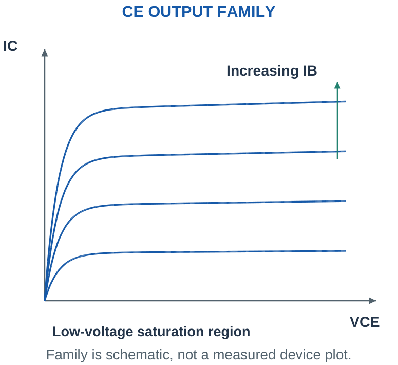
Cut-off lies near the zero-drive curve. At sufficiently high voltage, breakdown can occur outside the intended operating region. The graph in these notes identifies the useful regions without assigning an unspecified breakdown rating to every transistor.
The collector resistor and supply impose a load line. A device characteristic alone does not guarantee that any chosen IC and VCE pair can occur in the attached circuit. The operating point must satisfy both the transistor behaviour and external KVL/KCL equations.
Read the axes: A near-horizontal output curve is not a claim that the collector current can exceed the external circuit’s supply and load limit. A load line still constrains the point.
8. FIXED-BASE-BIAS CIRCUIT AND REGION CHECK
In a simple NPN stage, RC connects VCC to C, E returns to ground and RB connects a positive drive source to B. Assume forward active operation, calculate IB = (Vdrive – VBE)/RB, then IC = βIB and VC = VCC – IC RC. With E grounded, VCE = VC.
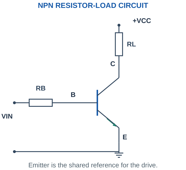
Now verify the assumption. Positive base current alone is insufficient: BC should remain reverse biased for the stated active model. If the calculation demands more collector current than the supply/load can support, use a saturation model and recalculate load current from IC ≈ (VCC – VCE,sat)/RC with the provided values.
A simplified two-state switch model can treat OFF and saturated ON directly. A transition or near-knee case requires a more detailed model rather than pretending the active and saturated approximations join with perfect physical accuracy at every point.
Working order: Base loop → active candidate → collector voltage → region check → alternative state if necessary. Include the checked state with the final current.
Worked check: Check a collector candidate
With VCC = 10 V, RC = 2 kΩ, supplied β = 100 and IB = 10 µA, the active candidate is IC = 1 mA and VC = 10 – 0.001 × 2,000 = 8 V. With VB = 0.7 V and grounded emitter, VC > VB supports the assumed reverse-biased BC condition.
Worked Problem 2.7: Calculate and Verify an Active Point
Problem: Vdrive = 5 V, RB = 100000 Ω, β = 100, VCC = 12 V and RC = 1000 Ω. E is grounded and VBE = 0.7 V. Find IC and VCE, then check active operation.
Model / approach: Assume forward active and verify VC exceeds VB.
Step 1: IB = (5 – 0.7)/100000 = 43 µA.
Step 2: IC = βIB = 4.3 mA.
Step 3: VC = VCE = 12 – IC × 1000 = 7.7 V. VC > VB = 0.7 V.
Answer: Active assumption consistent; IC ≈ 4.3 mA; VCE ≈ 7.7 V.
Check and interpretation: The collector voltage check prevents using active gain at an impossible load point. The supplied β and VBE are approximations for this exercise, not a guarantee for all transistors or operating conditions.
Worked Problem 2.8: Reject an Excessive Active-Current Demand
Problem: Vdrive = 5 V, RB = 2200 Ω, VCC = 12 V and RC = 1000 Ω. Active β = 100 would demand too much current. Use VBE,sat = 0.8 V and VCE,sat = 0.2 V, with supplied adequate-drive criterion IC/IB ≤ 10.
Model / approach: Solve the saturated load circuit and verify its base-drive criterion.
Step 1: IC,on = (12 – 0.2)/1000 ≈ 11.8 mA.
Step 2: IB = (5 – 0.8)/2200 ≈ 1.9091 mA.
Step 3: Forced ratio IC/IB ≈ 6.181, below the stated limit 10.
Answer: Saturated model supported; IC ≈ 11.8 mA; VCE = 0.2 V.
Check and interpretation: The load, rather than unrestricted multiplication by active β, fixes the ON current here. Adequate drive is checked using the criterion supplied in this exercise; a real device must meet its relevant conditions.
9. DC LOAD LINE AND QUIESCENT POINT
For a grounded emitter and collector resistor, VCE = VCC – IC RC. The load-line endpoints are VCE = VCC at IC = 0, and IC = VCC/RC at VCE = 0 in the ideal line construction. A real saturated endpoint includes its nonzero VCE,sat when that model is used.
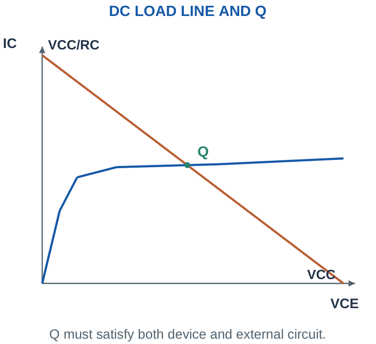
The quiescent point, Q, is the no-signal DC operating point. An amplifier is biased so the intended signal can vary around Q without repeatedly entering cut-off or saturation. A switch intentionally moves between different regions instead.
A midpoint collector voltage can provide useful approximate signal headroom in a simple resistively loaded stage. It is not an automatic rule for every topology or maximum-power design. Emitter voltage, load coupling, permitted distortion and actual transistor characteristics affect the useful swing.
Exam trick: Mark both load-line intercepts before Q. Then check VCC ≈ IC RC + VCE using the calculated point; this catches many resistor-unit and current-unit errors.
Worked Problem 2.9: Load-Line Intercepts and Q Point
Problem: A grounded-emitter stage has VCC = 12 V and RC = 2000 Ω. Its supplied Q current is 3 mA. Find line intercepts and VCEQ.
Model / approach: Use the ideal external line VCE = VCC – IC RC.
Step 1: At IC = 0, VCE = 12 V. At VCE = 0, IC = VCC/RC = 6 mA.
Step 2: At 3 mA, VCEQ = 12 – 0.003 × 2000 = 6 V.
Answer: Q = (6 V, 3 mA) using VCE, IC order.
Check and interpretation: The ideal intercept at VCE = 0 is a line-construction point. A real or supplied saturation model can have a nonzero minimum collector-emitter drop; the transistor characteristic must also support the intended Q region.
10. BJT AS A DIGITAL SWITCH
An NPN low-side switch places the load between the positive supply and collector, with the emitter connected to the return. A suitable input supplies base current through RB. Low drive gives cut-off; sufficient base drive can bring the transistor into saturation, placing most of the supply across the load.
With an illustrative saturated model, load current is (VCC – VCE,sat)/RL for a resistive load. Transistor conduction dissipation is approximately VCE,sat IC; base-drive power and switching transitions are separate contributions. OFF collector voltage can be near VCC while collector current is small, so OFF does not mean zero voltage across the device.
The load connected to the collector makes the collector voltage fall when the switch turns on. Thus an ON load and a LOW collector node can occur together. The meaning of HIGH/LOW must be tied to the measured node rather than the word ON alone.
Node trick: For a low-side NPN: base HIGH → transistor ON → collector LOW → load energised. The output node and load state should both be named.
Worked Problem 2.10: ON Current and Transistor Dissipation
Problem: A saturated NPN switches a 240 Ω load from 12 V. Use VCE,sat = 0.2 V. Find load current, switch loss and load power.
Model / approach: Steady resistive ON model; ignore base-power contribution in this collector-path balance.
Step 1: IC = (12 – 0.2)/240 ≈ 49.1667 mA.
Step 2: PQ = VCE,sat IC ≈ 9.8333 mW.
Step 3: Pload = IC²RL ≈ 0.5802 W; VCC IC ≈ 0.59 W.
Answer: IC ≈ 49.1667 mA; PQ ≈ 9.8333 mW.
Check and interpretation: Load power plus collector-path switch loss equals collector-supply power with unrounded values. This does not include base-drive loss or switching transitions, which need their own boundary and data.
11. BASE-RESISTOR DESIGN AND FORCED BETA
A switch-drive calculation often chooses a forced beta IC/IB smaller than the nominal active gain to provide adequate base drive under its stated conditions. A supplied forced beta of 10 means IB = IC/10; it does not mean every BJT has an intrinsic active gain of 10.
For required base current IB,min and supplied drive model, RB ≤ (Vdrive,min – VBE,max)/IB,min. If RB tolerance is t, its maximum actual value is Rnom(1 + t), so a nominal upper bound becomes (Vdrive,min – VBE,max)/[IB,min(1 + t)].
After choosing a resistor, recalculate both minimum and maximum base current. The driver must supply the current without violating its stated output conditions. A resistor satisfying base-current demand can still exceed a control pin’s allowed source current. A separate driver or another switching arrangement may then be needed.
Rounding trick: For a minimum base-current requirement, a larger RB can be the wrong direction. Solve the bound first. This differs from selecting a larger LED resistor to stay below a current ceiling.
Worked Problem 2.11: Design a Base Resistor
Problem: Required IC = 40 mA, chosen forced beta = 10, drive = 5 V and supplied VBE,sat = 0.8 V. Find RB upper bound and check 1000 Ω.
Model / approach: Required base current is IC divided by the chosen forced ratio.
Step 1: IB,min = 40/10 = 4 mA.
Step 2: RB,max = (5 – 0.8)/0.004 = 1050 Ω.
Step 3: For 1000 Ω, IB = 4.2 mA; achieved IC/IB ≈ 9.5238.
Answer: 1000 Ω meets the stated nominal minimum-base-current target.
Check and interpretation: Check whether the controller can deliver this current under its specified HIGH voltage. The chosen forced beta is a supplied switch-design target, not the nominal active gain or a universal saturation guarantee.
Worked Problem 2.12: Include Base-Resistor Tolerance
Problem: Required base current is 4 mA. Vdrive,min = 4.5 V, VBE,max = 0.9 V and RB tolerance is ±5%. Find maximum nominal RB and check 820 Ω.
Model / approach: Use maximum actual resistance for minimum current.
Step 1: Rnom ≤ (4.5 – 0.9)/(0.004 × 1.05) ≈ 857.1429 Ω.
Step 2: At 820 Ω nominal, Rmax = 861 Ω. IB,min = 3.6/861 ≈ 4.1812 mA.
Answer: 820 Ω passes the supplied minimum-current condition.
Check and interpretation: A nominal 900 Ω calculation would ignore tolerance. Maximum base current and driver capability must be checked separately at the opposite extremes.
Worked Problem 2.13: Driver-Current Limit
Problem: A relay needs 80 mA collector current and the exercise requires forced beta 10. The specified controller may source at most 4 mA at the required HIGH level. Can it directly meet the base-drive requirement?
Model / approach: Compare demanded base current with the supplied driver limit.
Step 1: IB,required = 80/10 = 8 mA.
Step 2: Available current is only 4 mA, so the direct-drive requirement is not met.
Answer: No: 8 mA is required, but only 4 mA is available.
Check and interpretation: Changing RB cannot create more valid source-current capability than the specified output provides. A suitable driver stage or another compatible switching arrangement is needed under these assumptions.
12. RELAY COIL DRIVER AND FLYBACK DIODE
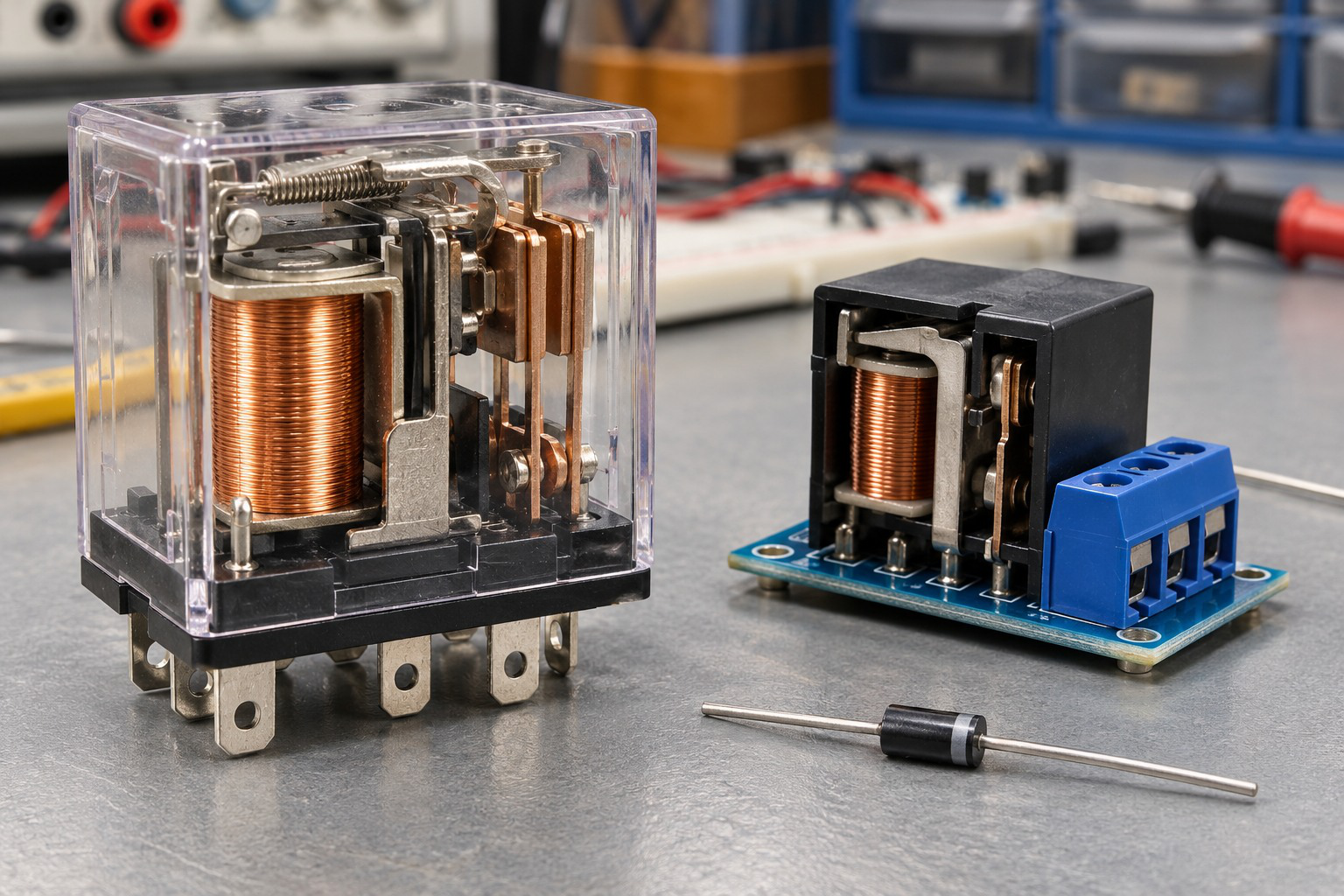
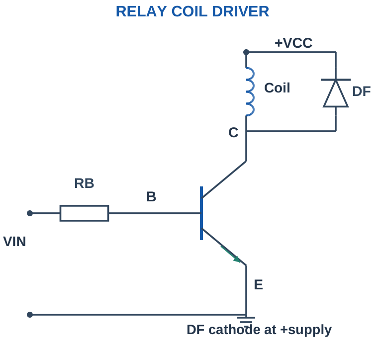
A relay coil is an inductive load. In a low-side NPN driver, the coil connects from +V to collector and the emitter returns to ground. A flyback diode connects across the coil with cathode at +V and anode at the collector. It is reverse biased during normal energisation.
TWO CIRCUITS IN A RELAY
| Coil Circuit | Contact Circuit |
|---|---|
| Energised by its driver | Switches the external load |
| Needs correct coil voltage/current | Needs suitable contact/load ratings |
| DC coil has a turn-off path | Separate inductive loads need their own analysis |
A flyback diode across the relay coil does not automatically suppress a different coil switched by its contacts.
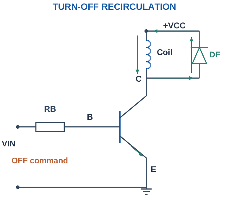
When the transistor turns off, coil current cannot disappear instantly. Its continuing current can flow from the coil’s lower end through the diode to the upper end, then through the coil in its original direction. This limits the collector voltage in the simple clamp arrangement. Inductor energy is E = ½LI² before turn-off.
Worked check: Flyback diode direction
In the illustrated low-side relay circuit, the diode anode is at collector and cathode at positive coil supply. During ON, collector is low and the diode blocks. After turn-off, the lower coil terminal rises enough to forward-bias it. Reversing the diode would make it conduct during the intended energised state, which is the wrong arrangement.
TURN-OFF CURRENT PATH
For the stated low-side DC coil: coil lower terminal → diode anode → diode cathode at +supply → coil upper terminal → coil lower terminal.
Coil current initially retains its direction. The switching node rises above the positive coil terminal to forward-bias the diode.
A simple diode clamp can make current decay and relay release slower than a higher-voltage clamp. Coil current, diode current, reverse voltage, switching rate and energy-handling conditions all belong to a real selection. The introductory circuit explains the mechanism without assigning one universal diode to every relay.
Polarity trick: Cathode to the positive coil supply. If the diode is forward biased during the intended ON state, the connection is wrong for this flyback arrangement.
Worked Problem 2.14: Relay Coil and Base-Drive Demand
Problem: A relay coil is modelled as 300 Ω on a 12 V supply. Use VCE,sat = 0.2 V, chosen forced beta 10, 5 V base drive and VBE,sat = 0.8 V. Find steady ON current and RB upper bound.
Model / approach: Use the supplied steady coil-resistance model, not an instantaneous turn-on-current prediction.
Step 1: IC ≈ (12 – 0.2)/300 = 39.3333 mA.
Step 2: IB,min = IC/10 = 3.9333 mA; RB,max = 4.2/IB ≈ 1067.7966 Ω.
Answer: Coil current ≈ 39.3333 mA; RB ≤ 1067.7966 Ω.
Check and interpretation: Inductance affects the current rise and turn-off behaviour. The flyback diode is reverse biased during the ON state and provides the recirculation path afterward; it is not part of the normal series base-current calculation.
Worked Problem 2.15: Stored Coil Energy
Problem: An ideal inductance L = 0.1 H carries 0.05 A just before switch-off. Find stored magnetic energy.
Model / approach: Use E = ½LI² for the supplied linear-inductor model.
Step 1: E = ½ × 0.1 × (0.05)² = 0.000125 J.
Step 2: In millijoules, E = 0.125 mJ.
Answer: Stored energy = 0.125 mJ.
Check and interpretation: This is the initial stored energy, not an automatic peak collector voltage. Voltage and decay time depend on the recirculation/clamp path, resistance and other circuit conditions.
Worked Problem 2.16: Simple Turn-Off Collector Clamp
Problem: A coil’s upper terminal is at 12 V and its lower terminal connects to an NPN collector. A flyback diode has cathode at 12 V and assumed forward drop 0.7 V. Estimate the collector voltage while the diode conducts after turn-off.
Model / approach: Use the illustrated low-side diode-clamp polarity.
Step 1: The collector/anode must rise about one diode drop above the cathode to conduct.
Step 2: VC ≈ 12 + 0.7 = 12.7 V in the idealised clamp model.
Answer: Collector clamp level ≈ 12.7 V.
Check and interpretation: The diode does not clamp the collector to 0.7 V relative to ground. Wiring inductance and switching transients can add stress in real circuits; this calculation identifies the nominal polarity and level.
13. BUZZER, LED AND RESISTIVE LOAD CONTROL
An active buzzer contains an internal oscillation mechanism and can produce its intended tone when supplied with suitable DC. A passive transducer normally needs a changing drive waveform for a sustained tone. Switching DC into both does not guarantee identical sound behaviour.
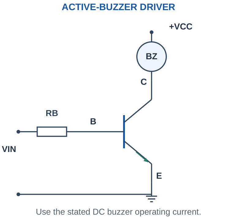
An LED load needs its own current-limiting resistor in the collector path. The base resistor limits base current; it is not the LED’s series current-limiting element. With a saturated switch, RLED = (VCC – VF,LED – VCE,sat)/ILED under the supplied constant-drop model.
Worked check: Two different resistor roles
An LED collector branch carrying 10 mA and a base branch carrying 1 mA need different resistor calculations. RLED is based on the supply minus LED and switch drops at 10 mA. RB is based on control voltage minus the base-emitter drop at 1 mA. Using either current in the other loop gives the wrong result.
TWO CIRCUITS IN A RELAY
| Coil Circuit | Contact Circuit |
|---|---|
| Energised by its driver | Switches the external load |
| Needs correct coil voltage/current | Needs suitable contact/load ratings |
| DC coil has a turn-off path | Separate inductive loads need their own analysis |
A flyback diode across the relay coil does not automatically suppress a different coil switched by its contacts.
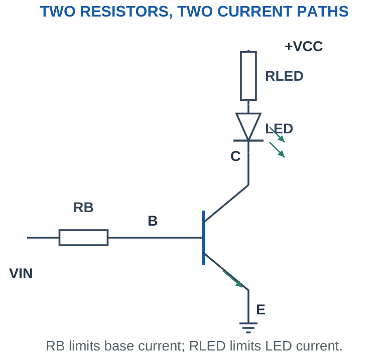
For an ordinary resistive load, the ON current follows its voltage and resistance. A buzzer or motor can have a nonresistive operating characteristic, so use the supplied operating current or model rather than replacing every load by the same resistor equation.
Worked Problem 2.17: LED Resistor in a Switched Collector Path
Problem: A saturated NPN drives an LED from 5 V. LED drop = 2 V, VCE,sat = 0.2 V and target ILED = 10 mA. Find ideal RLED.
Model / approach: Subtract both conducting drops from the collector-load supply.
Step 1: VRLED = 5 – 2 – 0.2 = 2.8 V.
Step 2: RLED = VRLED/0.01 = 280 Ω.
Answer: Ideal LED resistor = 280 Ω.
Check and interpretation: RB still serves the separate base path. Selecting an actual LED resistor requires recalculating its branch current and considering tolerance; the collector resistor is not found by dividing the supply by base current.
Worked Problem 2.18: Active Buzzer Load
Problem: An active buzzer is specified in this exercise to draw 25 mA at its intended operating point. A switch uses a supplied VCE,sat = 0.2 V. Estimate transistor collector-path dissipation.
Model / approach: Use the stated buzzer operating current rather than inventing a resistance.
Step 1: PQ ≈ VCE,sat IC = 0.2 × 0.025 = 0.005 W.
Step 2: The collector-path conduction loss is therefore 5 mW.
Answer: Approximate transistor conduction loss = 5 mW.
Check and interpretation: This does not determine the buzzer tone or prove a passive transducer will work from steady DC. Base drive and the intended buzzer supply voltage must still be consistent with the circuit.
14. DC MOTOR SWITCHING AND CURRENT
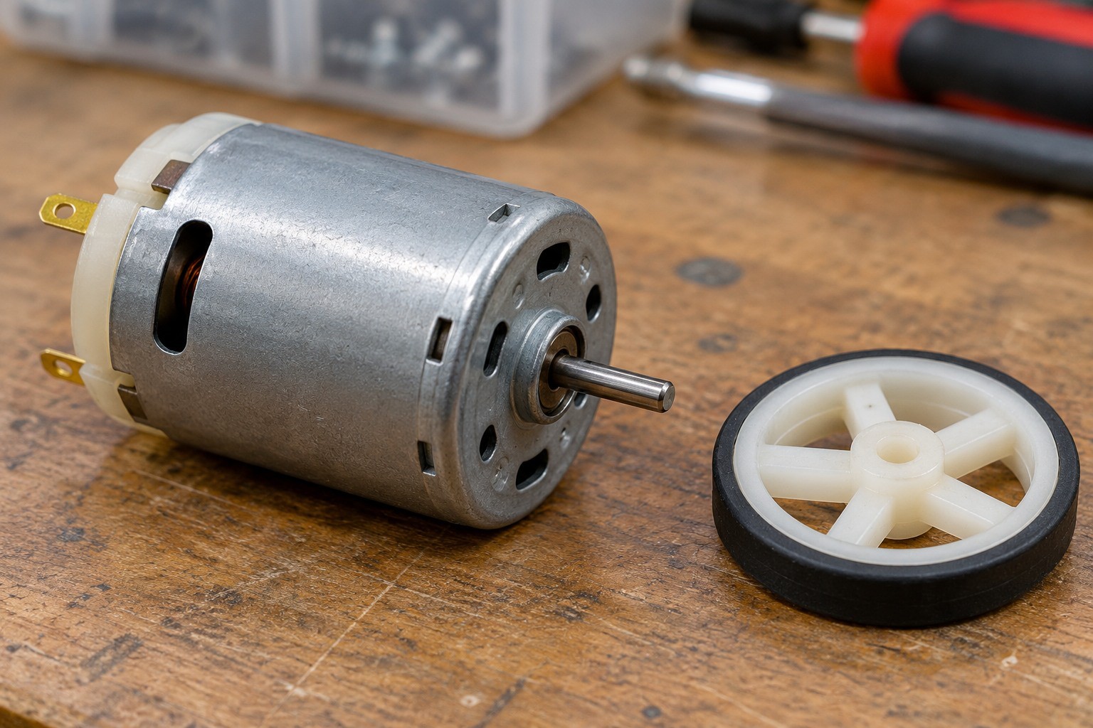
A DC motor is both an inductive and electromechanical load. Its current can be large at startup or stall because rotational back EMF is initially absent or small. In a supplied steady winding model, I ≈ (Vapplied – Eb)/R, where Eb is the opposing back EMF. At stall, Eb is approximately zero in that model.
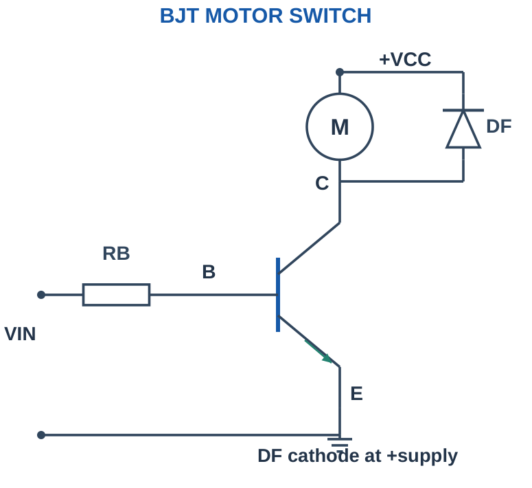
The switch must be assessed for the intended load current, voltage stress, switching conditions and heat dissipation. A calculation using a small running current alone does not describe the motor’s maximum demand. A saturated BJT also subtracts VCE,sat from the available motor voltage in the simple DC loop.
The control signal provides drive information and drive energy at its own terminal. Most motor energy comes from the motor supply through the load path. Share the appropriate reference for a non-isolated low-side arrangement rather than leaving the drive voltage undefined relative to the emitter/source.
Current trick: Do not select a drive only from “motor voltage.” Ask which current condition is supplied: running, startup or stall. Use the correct condition for the question.
Worked Problem 2.19: Running Current and Stall Current
Problem: Use the supplied steady motor model with applied winding voltage 6 V, resistance 2 Ω and running back EMF 4 V. Compare running current with the ideal stall case Eb = 0.
Model / approach: Use I = (V – Eb)/R; inductive transients and mechanical change are excluded.
Step 1: Running current = (6 – 4)/2 = 1 A.
Step 2: Stall-model current = 6/2 = 3 A.
Answer: 1 A running; 3 A idealised stall.
Check and interpretation: The difference shows why a small running current is not enough to describe the drive demand. The example uses a supplied steady model and does not claim current jumps instantly to the stall value at startup.
15. PNP SWITCHING AND POLARITY COMPARISON
A PNP can serve as a high-side switch with its emitter toward the positive supply and its collector feeding a load that returns to ground. Its base must be sufficiently below its emitter to turn on under the stated model. Bringing base near emitter turns it off.
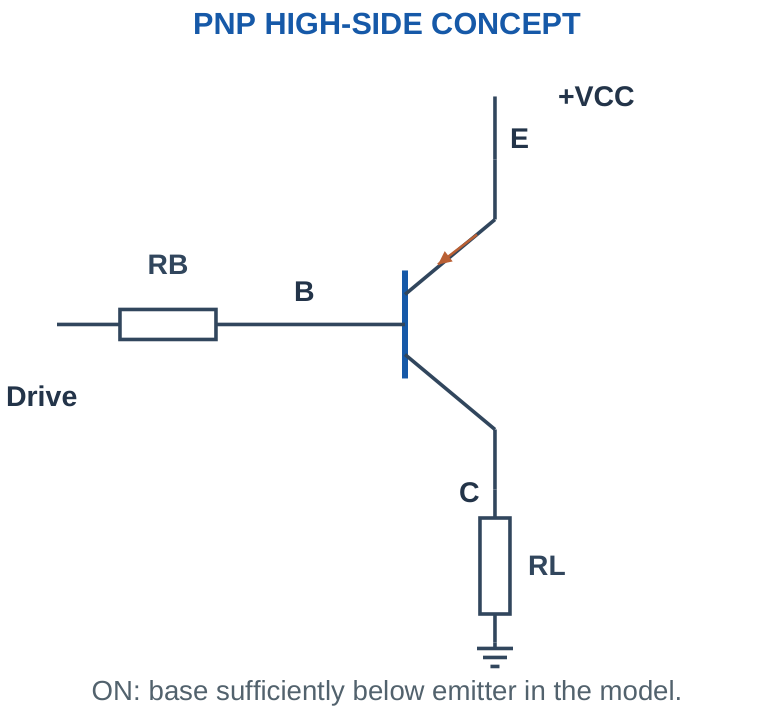
For a simple resistor-fed base pulled toward a lower voltage, use positive magnitudes with VEB = VE – VB. The base-current direction is opposite the usual NPN reference. An appropriately designed driver must be able to establish both ON and OFF conditions at the actual emitter voltage; a low-voltage logic signal is not automatically compatible with every higher supply.
Worked check: PNP voltage reference
If a PNP emitter is at 12 V and base at 11.2 V, VEB = 12 – 11.2 = 0.8 V. Using the NPN-style reference gives VBE = -0.8 V. Both describe the same terminal difference with opposite references. Do not interpret the negative VBE as proof that the correctly connected PNP must be OFF.
| Feature | Usual NPN Low Side | Usual PNP High Side |
|---|---|---|
| Main supply connection | Load above collector. | Emitter near positive supply. |
| ON base condition | Base above emitter. | Base below emitter. |
| OFF base condition | Base near emitter. | Base near emitter. |
Sign trick: Use one consistent voltage convention. For a PNP magnitude calculation, VEB is positive during the stated ON condition; do not insert it as an NPN VBE without changing signs.
Worked Problem 2.20: PNP Base-Current Magnitude
Problem: A PNP emitter is at 12 V. A resistor connects its base toward a 9 V drive node. Use VEB = 0.8 V while ON and RB = 2.2 kΩ. Find base-current magnitude.
Model / approach: Use PNP magnitudes: VB ≈ VE – VEB.
Step 1: VB ≈ 12 – 0.8 = 11.2 V.
Step 2: Resistor drop toward the 9 V node is 11.2 – 9 = 2.2 V. |IB| = 2.2/2,200 = 1 mA.
Answer: Base-current magnitude = 1 mA toward the lower-voltage drive.
Check and interpretation: The driving circuit must support the stated levels and current direction. The same resistor connected to an output that cannot establish the required OFF level would not guarantee a complete usable high-side driver.
16. COMMON-EMITTER AMPLIFIER PRINCIPLE
A CE amplifier uses a DC bias point in the forward-active region and a small input variation at the base. Increasing the input can increase base and collector current. The greater collector current produces a larger drop across RC, so collector voltage falls. This gives the familiar voltage inversion.
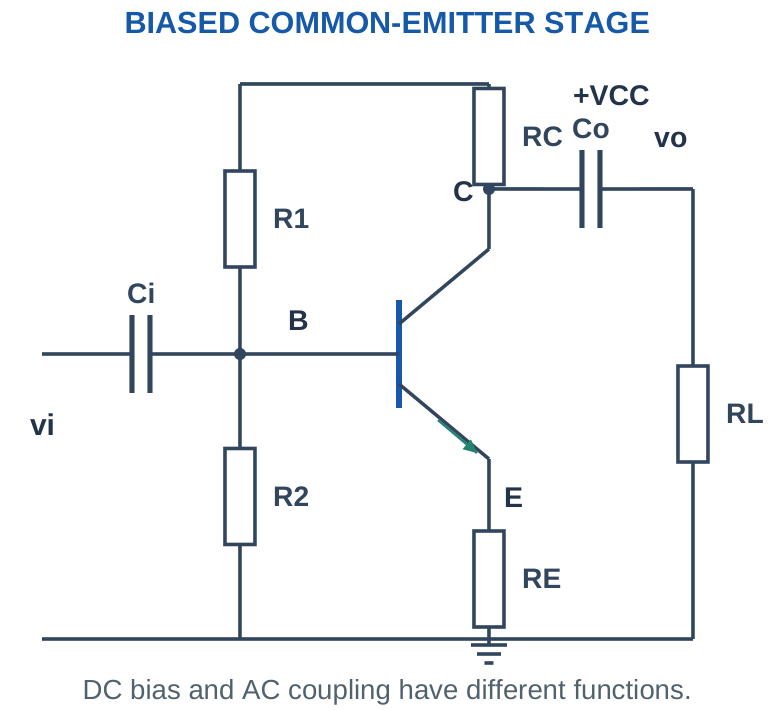
Voltage gain is Av = Δvo/Δvi or vo,ac/vi,ac under the stated small-signal conditions. A negative sign indicates inversion, not a negative amount of power. Current gain β is not the same as voltage gain Av. The external resistors, loading and emitter circuit strongly affect voltage gain.
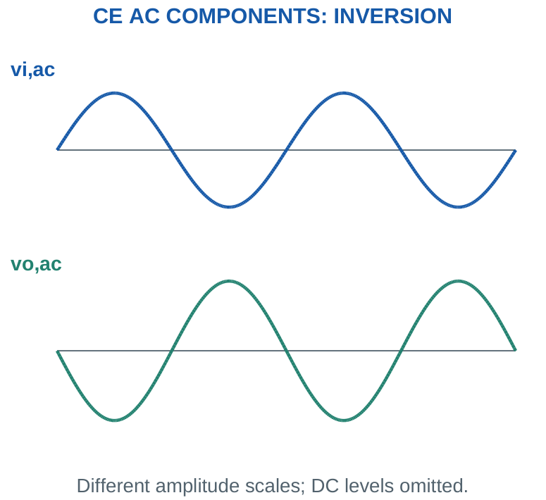
An amplifier’s output energy comes from its DC supply. The signal controls that energy transfer. It is therefore incorrect to say that a transistor creates energy simply because output signal amplitude is larger.
Answer pattern: Name the bias region, trace input increase → IC increase → RC drop increase → VC decrease, then define the signed gain and explain the supply’s role.
Worked Problem 2.21: Signed Voltage Gain
Problem: A CE stage has a small input change 10 mV and output change -0.3 V. Find voltage gain and describe the sign.
Model / approach: Use AC changes about the stated bias point, not absolute DC node voltages.
Step 1: Input = 0.01 V. Av = Δvo/Δvi = -0.3/0.01 = -30.
Step 2: The negative sign means the collector-output change is inverted relative to the input change.
Answer: Av = -30 V/V.
Check and interpretation: This gain is not β and is not a measure of power by itself. The stage must remain in its small-signal region for that ratio to describe an undistorted waveform.
17. DC BIAS AND EMITTER STABILISATION
A base voltage with an emitter resistor gives VE ≈ VB – VBE under the supplied conducting model. Then IE ≈ VE/RE and IC ≈ IE only when the large-beta approximation is explicitly accepted. For a stated finite β, IC = βIE/(β + 1).
A voltage-divider base network can be represented by VTH = VCC R2/(R1 + R2) and RTH = R1 || R2. Including base loading gives IB = (VTH – VBE)/[RTH + (β + 1)RE] in the assumed active model. From this, obtain IE, VE, IC, VC and VCE, then verify the region.
These are introductory bias calculations, not deep transistor design. The important point is that the DC circuit sets Q and the available signal swing. Coupling or bypass capacitors are open for the steady DC calculation in the usual ideal capacitor model.
Worked Problem 2.22: Emitter-Resistor Bias from a Fixed Base Voltage
Problem: Base is held at 1.7 V, VBE = 0.7 V, RE = 1000 Ω, β = 99, VCC = 12 V and RC = 2000 Ω. Find IE, IC and VCE.
Model / approach: Assume active operation; include the finite-beta current relationship.
Step 1: VE = 1.7 – 0.7 = 1 V; IE = VE/RE = 1 mA.
Step 2: IC = βIE/(β + 1) ≈ 0.99 mA.
Step 3: VC = 12 – IC × 2000 = 10.02 V; VCE = VC – VE = 9.02 V.
Answer: IC ≈ 0.99 mA; VCE ≈ 9.02 V.
Check and interpretation: VC remains above VB for the supplied values, consistent with reverse-biased BC. The fixed base source is an explicit assumption; an actual divider can be loaded by base current.
Worked Problem 2.23: Loaded Voltage-Divider Bias
Problem: VCC = 12 V. R1 = 47000 Ω from supply to base, R2 = 10000 Ω from base to return, RE = 1000 Ω, RC = 2200 Ω, β = 100, VBE = 0.7 V. Find the active-model Q point.
Model / approach: Replace the base divider by its Thevenin equivalent and include base loading.
Step 1: VTH = 2.1053 V; RTH = R1 || R2 = 8245.614 Ω.
Step 2: IB = (VTH – 0.7)/[RTH + (100 + 1)RE] = 12.8633 µA.
Step 3: IC = 1.2863 mA; VE = 1.2992 V; VC = 9.1701 V; VCE = 7.8709 V.
Answer: Q: IC ≈ 1.2863 mA, VCE ≈ 7.8709 V.
Check and interpretation: Check VC > VB using the unrounded values. Ignoring base loading would give a different estimate; the Thevenin equation makes that loading explicit under the supplied active model.
18. SMALL-SIGNAL GAIN WITH STATED MODELS
An optional introductory small-signal model uses gm ≈ IC/VT, with a supplied thermal voltage VT, and an emitter resistance re ≈ VT/IE. At room-temperature examples here use VT = 26 mV only when stated. These relations describe local behaviour around Q, not arbitrary large excursions between cut-off and saturation.
For a simple emitter-at-AC-ground CE stage, neglecting output resistance, Av ≈ -gm(RC || RL). An alternative approximate emitter-resistance form is Av ≈ -(RC || RL)/(re + RE,unbypassed), with the stated assumptions. They should not be mixed blindly when their parameter definitions differ.
Worked check: Gain is not beta
A supplied CE stage has β = 100 but measured voltage changes of +10 mV at input and -0.25 V at output. Its voltage gain is -25 V/V, not 100. Beta relates collector and base currents in its stated model; voltage gain depends on the surrounding signal circuit and load.
An emitter bypass capacitor can make an emitter resistor less significant to AC at suitable frequencies while leaving its DC bias role. At low enough frequency its impedance is not negligible, so a midband gain estimate is not a complete frequency-response curve.
Model trick: Write “small signal” and list the supplied assumptions. A very large computed gain does not guarantee a large undistorted output; Q and supply headroom still limit swing.
Worked Problem 2.24: Midband Gain with Collector Loading
Problem: Use IC = 1 mA, VT = 26 mV, RC = 2000 Ω and external AC load RL = 10000 Ω. Emitter is at AC ground and transistor output resistance is neglected. Find gm and Av.
Model / approach: Use gm = IC/VT and Av ≈ -gm(RC || RL).
Step 1: gm = 0.001/0.026 = 0.038461538 S.
Step 2: RC || RL = 1666.6667 Ω.
Step 3: Av ≈ -0.038461538 × 1666.6667 = -64.1026 V/V.
Answer: Midband gain ≈ -64.1026 V/V.
Check and interpretation: These are stated small-signal assumptions. Output swing must still fit around Q, and input/output coupling capacitors must behave as assumed over the signal frequency range.
Worked Problem 2.25: Unbypassed Emitter Resistance
Problem: Use IE = 1 mA, VT = 26 mV, effective collector AC load 2000 Ω and unbypassed emitter resistance 100 Ω. Estimate gain with the supplied emitter-resistance model.
Model / approach: Use re ≈ VT/IE and Av ≈ -RC,eff/(re + RE,u).
Step 1: re ≈ 0.026/0.001 = 26 Ω.
Step 2: Av ≈ -2000/(26 + 100) = -15.873 V/V.
Answer: Av ≈ -15.873 V/V.
Check and interpretation: The unbypassed emitter resistance reduces gain magnitude in this model and supports feedback. Do not use the bypassed-emitter formula while retaining an emitter resistor that the stated AC circuit leaves unbypassed.
19. LOADING, COUPLING AND SIGNAL SWING
A connected load can reduce the effective collector load from RC to RC || RL in the appropriate AC equivalent. This can reduce voltage-gain magnitude. The coupling capacitor ideally blocks DC while passing AC according to its impedance and the resistances it sees; it does not pass every frequency equally well.
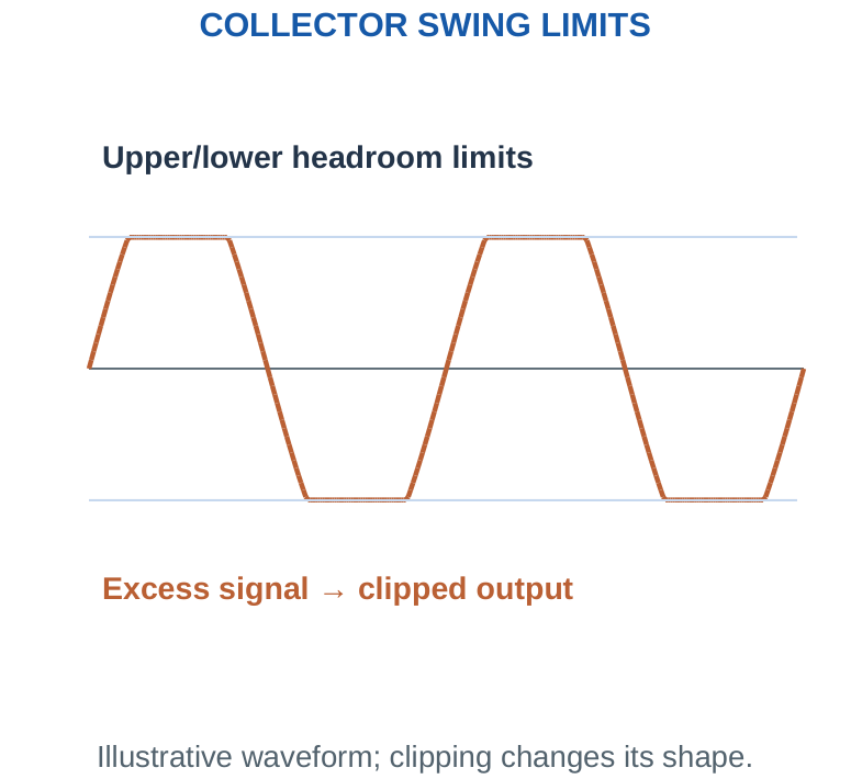
For a simple collector output with an approximately fixed emitter AC reference, upper output headroom is VCC – VCQ and lower headroom is VCQ – (VE + VCE,sat). The smaller value gives an approximate symmetric peak-swing limit before the model reaches one boundary. Real distortion can begin earlier.
Worked check: Peak swing check
A supplied linear gain is -50 and input peak is 20 mV. Output demand is 50 × 0.020 = 1 V peak. If the available symmetric output peak is only 0.8 V, the demand exceeds the stated limit. The nominal gain does not create more supply headroom; reduce the signal or change the appropriate design conditions.
Worked check: Peak-to-peak conversion
A sinusoidal output is 2 V peak-to-peak. Its peak is 1 V, and RMS is 1/√2 ≈ 0.7071 V. Across a stated 1 kΩ load, signal power is 0.7071²/1,000 = 0.5 mW. Treating the 2 V peak-to-peak value as RMS would overestimate that power by a factor of eight.
Peak/RMS trick: For a sine, Vpp = 2Vp and Vrms = Vp/√2. Use the output peak when checking headroom and RMS when calculating resistive signal power.
Worked Problem 2.26: Gain Reduction from a Load
Problem: A supplied CE small-signal model has gm = 0.04 S and RC = 2 kΩ. Compare gain with no external load and with RL = 2 kΩ, neglecting transistor output resistance.
Model / approach: Emitter is at AC ground in both cases.
Step 1: Unloaded Av ≈ -0.04 × 2,000 = -80.
Step 2: With RL, effective resistance = 2,000 || 2,000 = 1,000 Ω; Av ≈ -40.
Answer: Gain magnitude changes from 80 to 40.
Check and interpretation: The connected load changes the AC circuit even if DC bias is preserved by an ideal coupling capacitor. A no-load gain specification is not automatically the loaded stage gain.
Worked Problem 2.27: Output Headroom and Maximum Input Estimate
Problem: Use VCC = 12 V, VCQ = 6 V, fixed emitter AC reference VE = 1 V, lower limit VE + VCE,sat with VCE,sat = 0.2 V, and small-signal Av = -20. Estimate symmetric output peak and input peak before that limit.
Model / approach: Use the supplied simplified collector-swing bounds; real distortion can begin earlier.
Step 1: Upward headroom = 12 – 6 = 6 V.
Step 2: Downward headroom = 6 – (1 + 0.2) = 4.8 V; choose the smaller: 4.8 V peak.
Step 3: Input peak ≈ 4.8/20 = 240 mV.
Answer: Output peak limit ≈ 4.8 V; input peak ≈ 240 mV.
Check and interpretation: This checks a stated amplitude boundary, not a guarantee of zero distortion at the exact limit. Use peak values for clipping and RMS values for sinusoidal resistive power.
20. CLASS-A AUDIO AMPLIFICATION
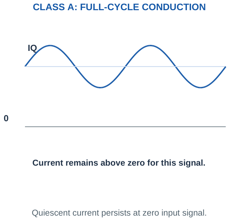
A class-A stage conducts throughout the full signal cycle, nominally 360°. Its transistor is biased so the intended waveform can vary about Q while remaining in the usable amplifying region. It is not a switch spending most of its time alternately in cut-off and saturation.
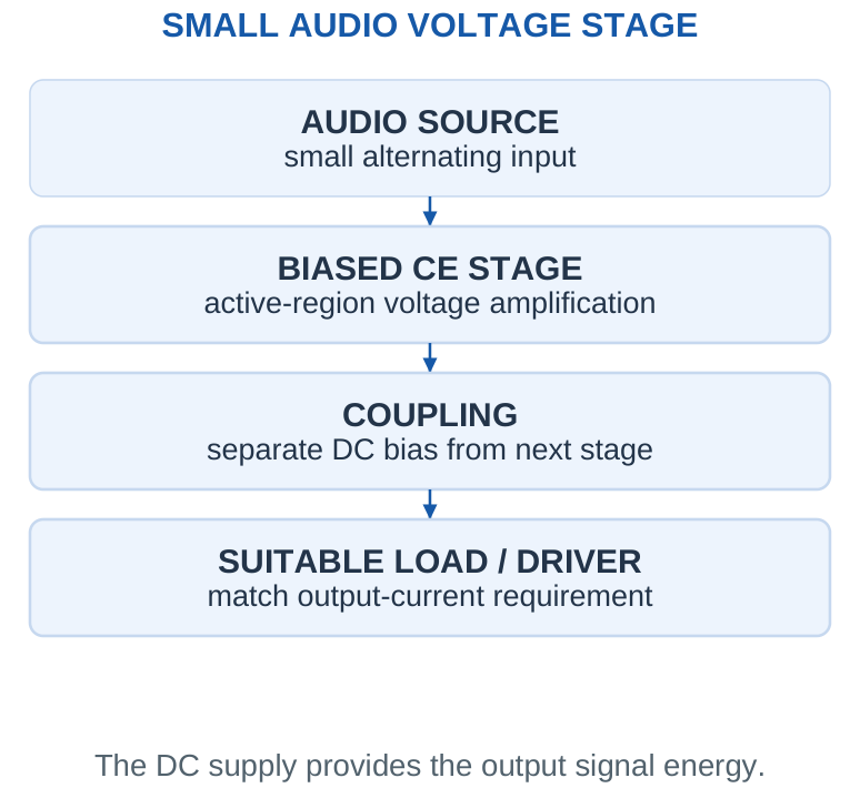
A small CE stage can amplify an audio voltage for a following circuit. Its collector output is inverted and often AC coupled to avoid passing its DC bias to the next stage. A small voltage-amplifier transistor stage is not automatically able to drive a low-resistance loudspeaker directly; load demand and output-drive capability must be considered.
Worked check: Full-cycle class-A current
A supplied class-A current is iC = 3 mA + 1 mA sin θ. It varies from 2 to 4 mA and stays positive throughout the cycle. That supports the stated full-cycle conduction picture. It does not alone prove the collector-voltage swing remains within active-region limits; both current and voltage conditions matter.
GAIN AND SWING ARE SEPARATE
Gain: Small-signal output change divided by input change.
Bias: DC operating point about which the signal varies.
Headroom: Allowable positive and negative output changes.
Power: Use the actual load and RMS signal value.
A large calculated gain does not guarantee that the required output waveform fits without clipping.
For a stated sinusoidal signal across RL, output signal power is Vrms²/RL. DC input power to a simplified stage can be VCC ICQ when the problem defines that boundary and neglects other bias currents. Efficiency requires compatible input/output power definitions; the no-signal dissipation remains significant in a class-A stage.
Worked Problem 2.28: Sinusoidal Output Power
Problem: A stated undistorted sinusoidal output of 1 V peak appears across 1000 Ω. Find RMS voltage and average signal power in the resistor.
Model / approach: Use the sine relation Vrms = Vp/√2, not Vp as an RMS value.
Step 1: Vrms = 1/√2 ≈ 0.7071 V.
Step 2: Psignal = Vrms²/R = 0.5 mW.
Answer: Vrms ≈ 0.7071 V; signal power ≈ 0.5 mW.
Check and interpretation: The result describes the supplied output waveform and load. It does not prove the transistor stage can provide that swing or current; those capabilities must already be consistent with bias and the connected circuit.
Worked Problem 2.29: DC Input and Signal Efficiency
Problem: A supplied class-A stage boundary uses VCC = 10 V and ICQ = 5 mA, neglecting other bias currents. Measured useful AC load power is 8 mW. Find approximate DC input and efficiency.
Model / approach: Use matching input/output power definitions for this exercise.
Step 1: PDC ≈ 10 × 0.005 = 50 mW.
Step 2: η = 8/50 × 100 = 16%.
Answer: DC input ≈ 50 mW; signal efficiency ≈ 16%.
Check and interpretation: The quiescent input does not disappear when the small audio signal becomes zero. This calculation does not assign the same efficiency to every class-A topology or every signal level.
21. INTRODUCTION TO FIELD-EFFECT TRANSISTORS
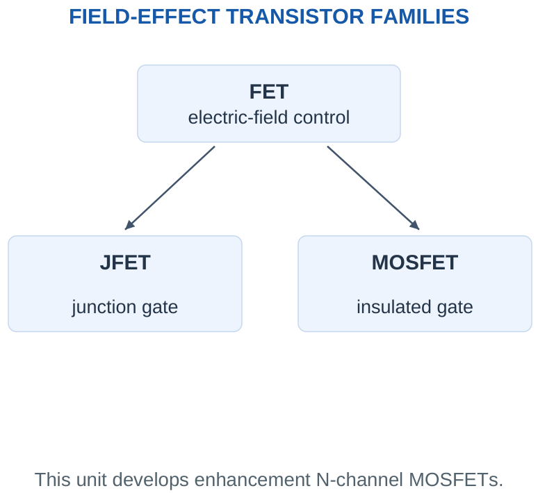
A field-effect transistor controls a conducting channel using an electric field associated with a gate voltage. The usual terminal names are gate G, drain D and source S. JFETs use a junction-controlled gate structure; MOSFETs use an insulating gate structure. Do not assume their zero-bias states and gate connections are interchangeable.
In a MOSFET, the insulated gate draws very small steady leakage current in the simplified DC view, but its capacitances must be charged and discharged during transitions. “Voltage controlled” therefore does not mean a real switching driver supplies no current at any time.
| BJT Introductory View | MOSFET Introductory View |
|---|---|
| Base drive current supports collector action. | Gate-to-source voltage controls the channel. |
| Base current often persists while ON. | Gate charging current is mainly transient, with leakage in steady state. |
| Three main terminals B/C/E. | Three commonly used terminals G/D/S, plus body connection. |
Terminal trick: The gate voltage must be measured relative to source. Ground-relative gate voltage is sufficient only when source is actually at that ground reference.
22. ENHANCEMENT N-CHANNEL MOSFET
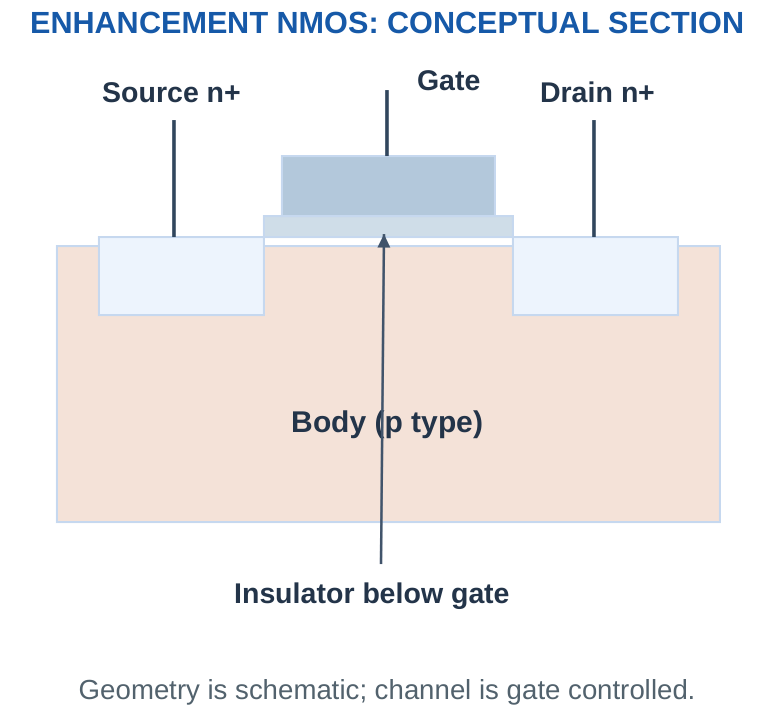
An enhancement N-channel MOSFET forms a conducting channel under an appropriate positive gate-to-source voltage. In the elementary zero-bias picture it is normally OFF at VGS = 0. Its gate is separated from the semiconductor by an insulating layer, so voltage can establish an electric field without an intended continuous conducting gate path.
GATE-DRIVE CHECKLIST
Reference: Subtract VS from VG.
Steady ON: Use RDS,on at stated drive and temperature.
Transition: Supply and remove gate charge.
OFF: Consider pull-down and body-diode direction.
Threshold, low ON resistance and switching speed describe different conditions.
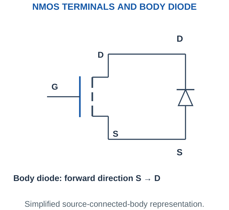
Discrete power MOSFETs often connect body to source internally, producing an intrinsic body-diode relationship. In a usual N-channel low-side arrangement, that diode’s forward direction is from source to drain. The device is not simply a symmetric ideal resistor that blocks both polarities when OFF.
Worked check: Capacitive gate example
For an explicitly supplied ideal gate capacitance of 500 pF and a 5 V change, Q = CΔV = 500 × 10^-12 × 5 = 2.5 nC. This is a capacitor-model exercise. A real MOSFET’s total gate charge at a specified drain operating condition need not equal one constant capacitance times drive voltage.
GATE-DRIVE CHECKLIST
Reference: Subtract VS from VG.
Steady ON: Use RDS,on at stated drive and temperature.
Transition: Supply and remove gate charge.
OFF: Consider pull-down and body-diode direction.
Threshold, low ON resistance and switching speed describe different conditions.
Construction explains the high DC input impedance and the need to control gate voltage and transient charge. Detailed fabrication and square-law derivations are beyond the required introductory scope; use supplied models when doing numerical exercises.
23. VGS, THRESHOLD AND ADEQUATE GATE DRIVE
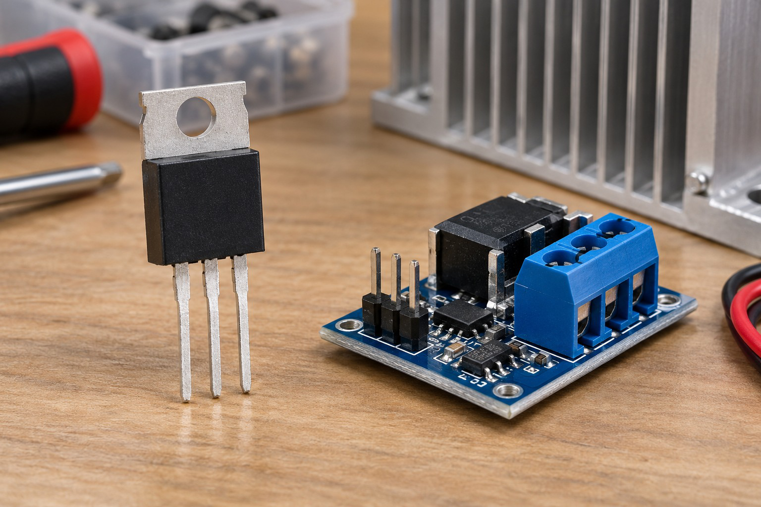
Define VGS = VG – VS. A gate at 5 V with its source at 4.5 V has only 0.5 V gate-to-source drive. A gate voltage stated relative to ground cannot be used as VGS without checking the source potential.
Worked check: Source movement changes drive
A gate remains at 5 V while source rises from 0 to 3.5 V. VGS falls from 5 V to 1.5 V. The controller’s ground-relative HIGH has not changed, but the device drive condition has. This is why a low-side source-reference assumption cannot be silently transferred to a moving-source high-side arrangement.
Worked check: Threshold is a test condition
A hypothetical part has a threshold measured at 250 µA. A load requires 2 A, which is 8,000 times that test current. The threshold does not prove the channel has its desired low resistance at 2 A. Use the relevant ON-resistance condition at the available VGS rather than extending the tiny-current definition.
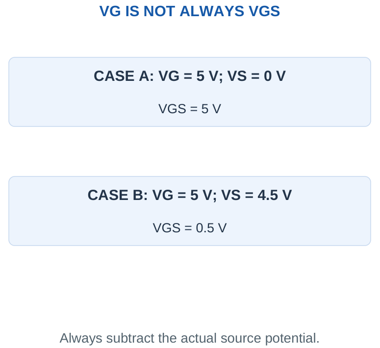
VGS,th describes a threshold condition at a specified small drain current, not a universal voltage that guarantees the required low ON resistance at a large load current. Use an RDS,on specification or supplied model at the actual intended gate drive and relevant temperature. A specification at 10 V does not automatically establish the same resistance at 3.3 V.
A logic-level label should be interpreted through the required operating data, not merely through the numerical threshold. For introductory exercises, use a clearly supplied resistance at the stated VGS. This avoids inventing actual component performance from an unspecified threshold.
Exam trap: “VGS exceeds threshold” and “MOSFET is adequately enhanced for the load” are different claims. Check the required load current and specified ON resistance at the available drive.
Worked Problem 2.30: Gate Voltage Is Relative to Source
Problem: A MOSFET gate is at 5 V and source at 0 V relative to the same ground. Find VGS. Can a ground-relative gate number alone establish full enhancement?
Model / approach: Use VGS = VG – VS.
Step 1: VGS = 5 – (0) = 5 V.
Step 2: Adequate ON resistance must be assessed at this gate-to-source value using the supplied operating data, not merely the ground-relative gate voltage.
Answer: VGS = 5 V; full enhancement needs appropriate additional data.
Check and interpretation: A positive gate-to-ground voltage can still give very small VGS when source is high. Threshold alone is not enough to guarantee a useful low-loss state at the required load current.
Worked Problem 2.31: Gate Voltage Is Relative to Source
Problem: A MOSFET gate is at 3.3 V and source at 1.8 V relative to the same ground. Find VGS. Can a ground-relative gate number alone establish full enhancement?
Model / approach: Use VGS = VG – VS.
Step 1: VGS = 3.3 – (1.8) = 1.5 V.
Step 2: Adequate ON resistance must be assessed at this gate-to-source value using the supplied operating data, not merely the ground-relative gate voltage.
Answer: VGS = 1.5 V; full enhancement needs appropriate additional data.
Check and interpretation: A positive gate-to-ground voltage can still give very small VGS when source is high. Threshold alone is not enough to guarantee a useful low-loss state at the required load current.
24. MOSFET REGIONS AND THE SATURATION TRAP
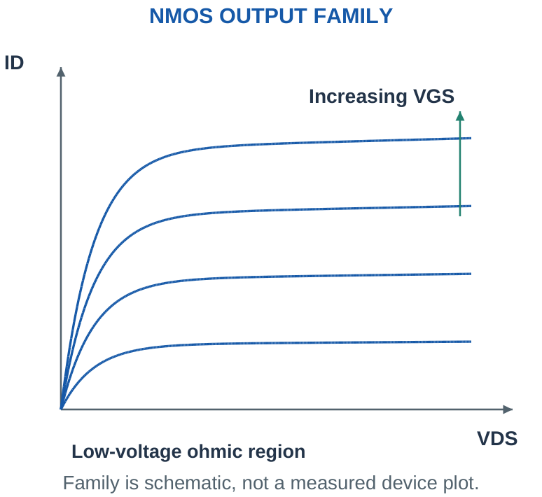
For an elementary enhancement NMOS model, cut-off occurs below the stated threshold condition. With VGS above threshold, the device can operate in the linear/ohmic region at sufficiently small VDS or in the saturation region at a larger VDS. In a long-channel textbook model, the boundary is approximately VDS = VGS – Vth.
| Device | Commonly Desired Low-Loss ON-Switch Description |
|---|---|
| BJT | Saturation with small VCE,sat under adequate base drive. |
| MOSFET | Adequately enhanced low-RDS,on/ohmic operation. |
MOSFET saturation is associated with a channel condition useful for current-source-like or amplifying behaviour in the elementary model. It is not the same as BJT saturation. Power devices have further practical effects, so the simple boundary is used only as a stated model in introductory region questions.
Naming trick: Memorise the distinction before comparing graphs: BJT saturation → ON-switch example; MOSFET ohmic region → ON-switch example. The same region word cannot be transferred between devices without its definition.
Worked Problem 2.32: Classify a Supplied Textbook MOSFET Model
Problem: For an enhancement NMOS model, VGS = 5 V, Vth = 2 V and VDS = 0.2 V. Use the stated long-channel boundaries to identify the region.
Model / approach: First compare VGS with Vth, then compare VDS with VGS – Vth when above threshold.
Step 1: VGS – Vth = 5 – 2 = 3 V.
Step 2: Under these supplied boundaries, the operating point is ohmic/linear.
Answer: Ohmic/linear in the specified model.
Check and interpretation: This is a region-classification exercise, not a calculation of a real power MOSFET rating. The MOSFET word saturation must not be interpreted as the same low-drop switch state used for a saturated BJT.
25. N-CHANNEL LOW-SIDE MOSFET SWITCH
The load connects between +V and drain, source returns to ground, and gate is driven relative to source. A suitable gate-source pull-down gives a defined OFF tendency when the driver is disconnected or high impedance. A series gate resistor can shape the transient gate current, but it is not a DC load-current resistor.
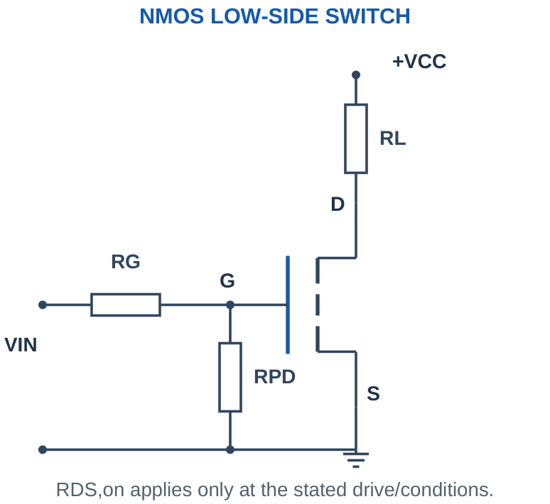
With supplied ON resistance r, the conducting device has VDS ≈ ID r and conduction loss ≈ ID²r. If the load is a resistor RL, its current is VSUP/(RL + r) under the simple steady ON model. Treating VDS as a fixed 0.2 V would be a BJT-style assumption unless a problem explicitly supplies that MOSFET model.
When OFF, the gate is approximately at source potential and the drain can rise toward the supply through the load. A low gate current in the DC model does not establish adequate switching speed; gate charge and driver capability matter during changes.
Connection trick: Source at the return, drain at the load, and gate referenced to source in this low-side example. Do not reverse source and drain casually: the body diode changes the OFF-state behaviour.
Worked Problem 2.33: Resistive Load with Finite ON Resistance
Problem: An adequately driven NMOS has supplied RDS,on = 0.05 Ω. It switches a 6 Ω resistor from 12 V. Find current, MOSFET drop and conduction loss. For the illustrated drive, VIN = 5 V and RG = 100 Ω; the supplied ON resistance applies at that drive.
Model / approach: Use a series RL + RDS,on steady ON model.
Step 1: ID = 12/(6 + 0.05) ≈ 1.9835 A.
Step 2: VDS,on = ID RDS,on ≈ 0.0992 V.
Step 3: PQ = ID²RDS,on ≈ 0.1967 W.
Answer: ID ≈ 1.9835 A; PQ ≈ 0.1967 W.
Check and interpretation: The supplied resistance must apply at the intended drive and conditions. The current differs slightly from supply/RL because the switch has a nonzero ON drop; load plus switch power balances source input in this model.
26. ON RESISTANCE, LOSSES AND TEMPERATURE
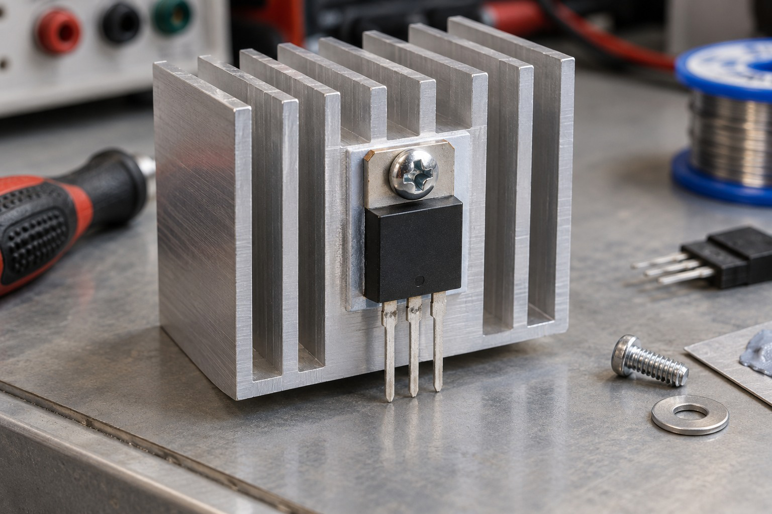
A MOSFET’s conduction loss depends on current squared and the relevant ON resistance. If the supplied resistance increases with temperature, calculate loss at that increased value for the stated current. A single maximum current rating alone does not establish how hot a device will run on a particular board.
For a supplied thermal resistance θ and dissipation P under its applicable steady conditions, ΔT ≈ Pθ and Tj ≈ Ta + ΔT. This is a simplified estimate; transient, mounting and cooling conditions can change the relevant thermal model. Use only the thermal values actually supplied in a problem.
Switching loss is separate from steady conduction loss. An approximate hard-switching overlap model is Psw ≈ ½V I(tr + tf)f for its stated assumptions. It is included as optional arithmetic enrichment, not as a complete model of every converter or motor drive.
Square-law arithmetic trick: With resistance fixed, doubling current multiplies conduction loss by four. Do not confuse this I²R relation with a claim that every MOSFET’s current-voltage characteristic is a fixed square law.
Worked Problem 2.34: Conduction Loss at a Stated Current
Problem: A supplied ON resistance is 0.05 Ω at the relevant operating condition and current is 2 A. Find ON voltage drop and conduction loss.
Model / approach: Use the given resistance and steady current; switching transitions are excluded.
Step 1: VDS = ID RDS,on = 2 × 0.05 = 0.1 V.
Step 2: Pcond = ID²RDS,on = 2² × 0.05 = 0.2 W.
Answer: VDS = 0.1 V; loss = 0.2 W.
Check and interpretation: If current doubles while resistance stays fixed, drop doubles but loss quadruples. A quoted resistance from another drive voltage or temperature cannot automatically be substituted for the relevant operating value.
Worked Problem 2.35: Temperature-Related Resistance Rise
Problem: At a supplied 25°C reference, RDS,on = 0.04 Ω. The exercise specifies a hot-condition multiplier of 1.5 and current 3 A. Compare losses.
Model / approach: Use the supplied resistance multiplier rather than inventing a universal temperature coefficient.
Step 1: Hot resistance = 0.04 × 1.5 = 0.06 Ω.
Step 2: Reference loss = 3² × 0.04 = 0.36 W; hot loss = 3² × 0.06 = 0.54 W.
Answer: Loss rises from 0.36 to 0.54 W at the same supplied current.
Check and interpretation: The multiplier is specific problem data. This is not a self-consistent electrothermal solution; a real temperature rise can feed back into resistance and depends on the actual mounting and heat paths.
27. GATE CHARGE AND DRIVER CURRENT
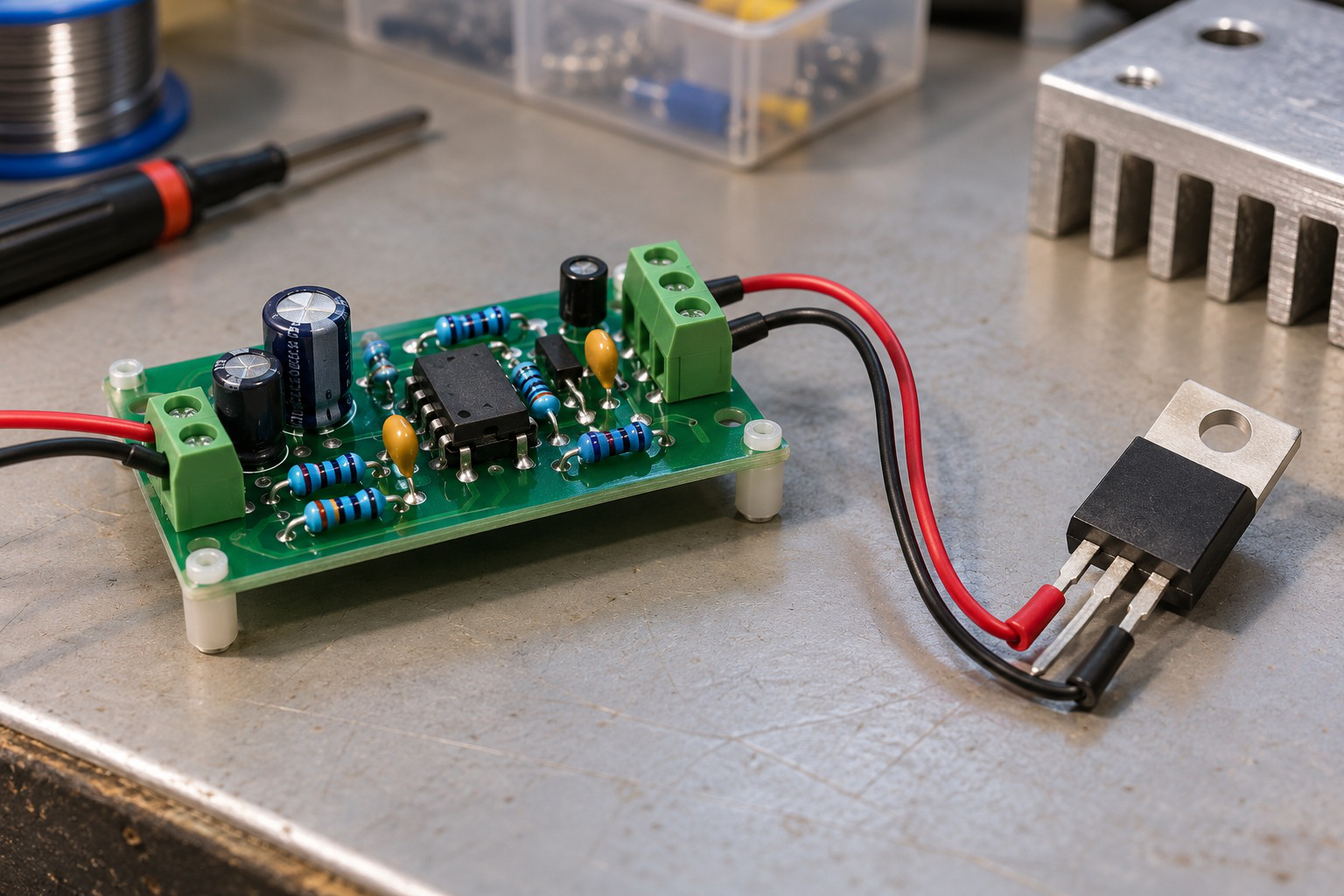
The gate behaves capacitively during a transition. A driver supplies charge to raise its voltage and removes charge to lower it. A supplied total gate charge Qg and switching frequency f give an average charging-current estimate Iavg ≈ Qg f, while an idealised constant transition current gives t ≈ Q/I.
Worked check: Average versus pulse current
A supplied 20 nC gate-charge interval repeated at 5 kHz requires an average charging current of Qf = 0.10 mA. If that same charge is moved in 1 µs with a constant-current approximation, the interval current is 20 mA. Small average demand does not imply equally small transition current.
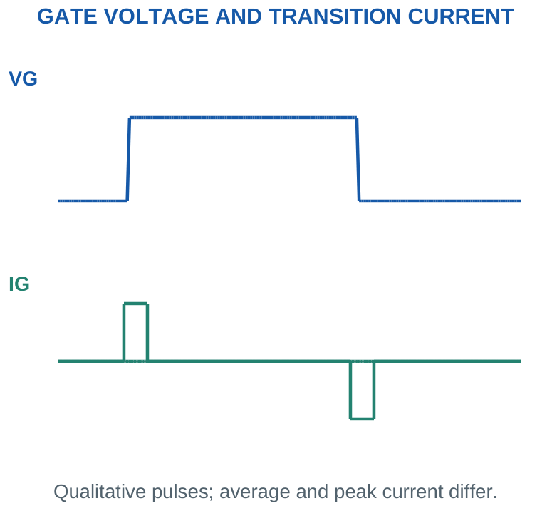
A rough gate-drive energy-per-cycle estimate is Qg Vdrive, giving Pgate ≈ Qg Vdrive f under the stated model. The detailed division of energy between driver resistances and device paths is not represented by treating all of it as MOSFET drain-channel heat.
Real gate charge depends on the operating conditions and includes voltage intervals affected by gate-drain coupling. A single C times V model can be useful when explicitly supplied, but is not automatically interchangeable with a gate-charge value under every condition.
Current trick: Tiny steady gate current does not mean zero driver demand. Distinguish steady leakage, average charging current and peak transition current before evaluating a logic output.
Worked Problem 2.36: Average Charging Current and Drive Power
Problem: Total gate charge is supplied as 20 nC for the stated transition conditions. Switching frequency is 10 kHz and drive amplitude 5 V. Estimate average charging current and idealised gate-drive power.
Model / approach: Use Iavg ≈ Qg f and Pgate ≈ Qg Vdrive f.
Step 1: Iavg = 20 × 10^-9 × 10000 = 0.2 mA.
Step 2: Pgate ≈ Iavg Vdrive = 1 mW.
Answer: Average charging current ≈ 0.2 mA; drive power ≈ 1 mW.
Check and interpretation: Short transition currents can be much larger than the average. Do not add all gate-drive power to drain-channel dissipation without defining where that energy is dissipated.
28. PWM: DUTY CYCLE, PERIOD AND WAVEFORM
Pulse-width modulation changes the proportion of each repeated period for which the switch is ON. Duty cycle D = ton/T and switching frequency f = 1/T. Changing duty at fixed frequency changes pulse width; changing frequency at fixed duty changes both ON and OFF durations proportionally.
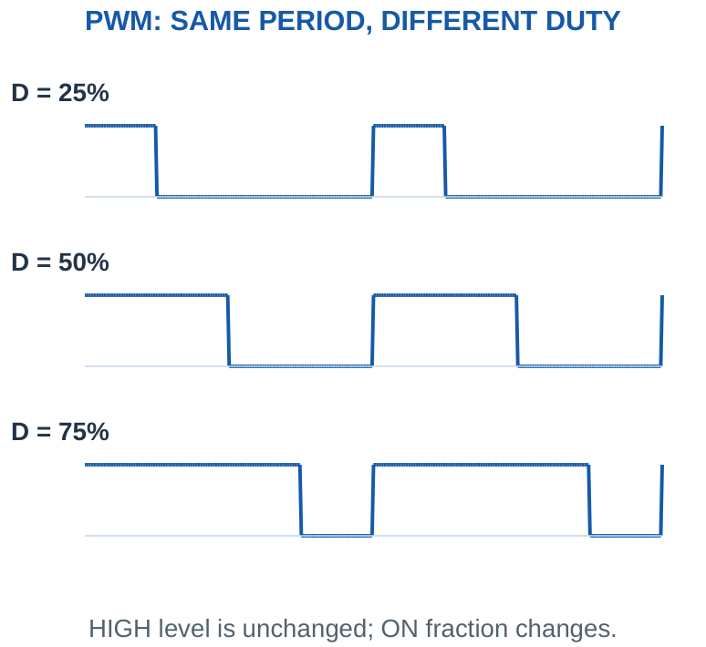
For an ideal 0-to-V pulse waveform, average voltage is DV and RMS voltage is V√D. These are different. Across a purely resistive load, average heating power is DV²/R. Using (DV)²/R would underestimate that heating except at D = 0 or 1 because it incorrectly treats the average as a steady voltage with the same RMS.
A motor is not merely that resistor. Its current depends on inductance, back EMF, speed and the recirculation path. Duty controls the drive pattern, but actual motor speed and current are not universally equal to duty times a single maximum value.
Duty trick: Convert a percentage to a fraction before calculation: 30% means D = 0.30. PWM changes time fraction, not the logic-HIGH amplitude itself.
Worked Problem 2.37: PWM Period, ON Time and OFF Time
Problem: PWM frequency is 1000 Hz and duty is 25%. Find period, ON time and OFF time.
Model / approach: Use D = ton/T and T = 1/f; convert the percentage to a fraction.
Step 1: T = 1/1000 = 1000 µs.
Step 2: ton = 0.25T = 250 µs.
Step 3: toff = (1 – 0.25)T = 750 µs.
Answer: T = 1000 µs; ton = 250 µs; toff = 750 µs.
Check and interpretation: ON and OFF times add to one period. Changing duty at a fixed frequency changes the pulse width, not the intended HIGH-level amplitude.
Worked Problem 2.38: Average Versus RMS and Resistive Heating
Problem: An ideal 0-to-12 V PWM waveform has duty 25% across 12 Ω. Find average voltage, RMS voltage and average resistor power.
Model / approach: The load is explicitly resistive; this is not a motor-current calculation.
Step 1: Vavg = DV = 3 V.
Step 2: Vrms = V√D = 6 V.
Step 3: Pavg = Vrms²/R = DV²/R = 3 W.
Answer: Vavg = 3 V; Vrms ≈ 6 V; Pavg = 3 W.
Check and interpretation: Using Vavg²/R would treat the pulsed waveform as steady DC and gives the wrong heating. A motor needs its inductive/electromechanical model rather than this pure-resistor substitution.
29. MOSFET PWM MOTOR CONTROL
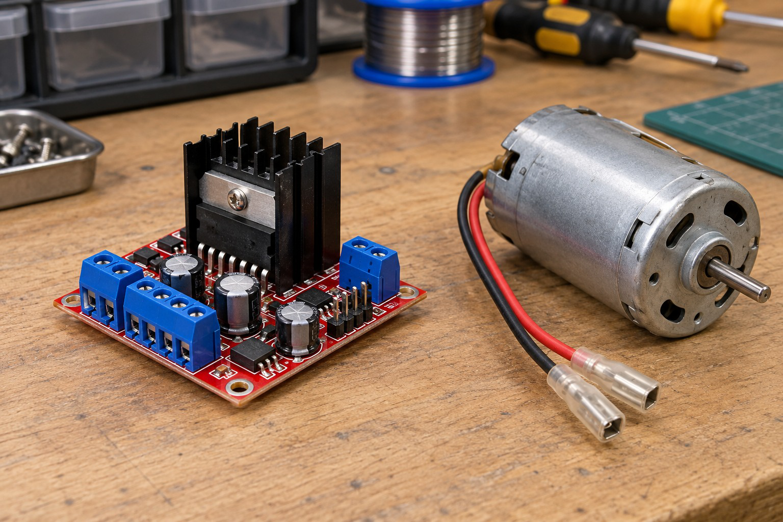
In a basic low-side NMOS motor driver, the motor connects from supply to drain and a recirculation diode connects across it with cathode toward supply. The gate receives the intended PWM drive. During ON time, supply energy flows through motor and MOSFET. During OFF time, winding current can recirculate through the diode under the stated operating condition.
Worked check: Body diode versus recirculation diode
In the illustrated low-side N-channel arrangement, the intrinsic body diode points from source toward drain. At turn-off the motor can drive drain above the positive supply; that diode is not forward oriented to return current from drain to the upper motor terminal. The external motor diode provides the intended loop.
Worked check: Duty and ON amplitude
For ideal 12 V pulses, duty changing from 25% to 75% changes average voltage from 3 to 9 V. The pulse amplitude remains 12 V. This explains the timing control but does not by itself establish a motor’s speed or current, which also depend on its load and electrical behaviour.
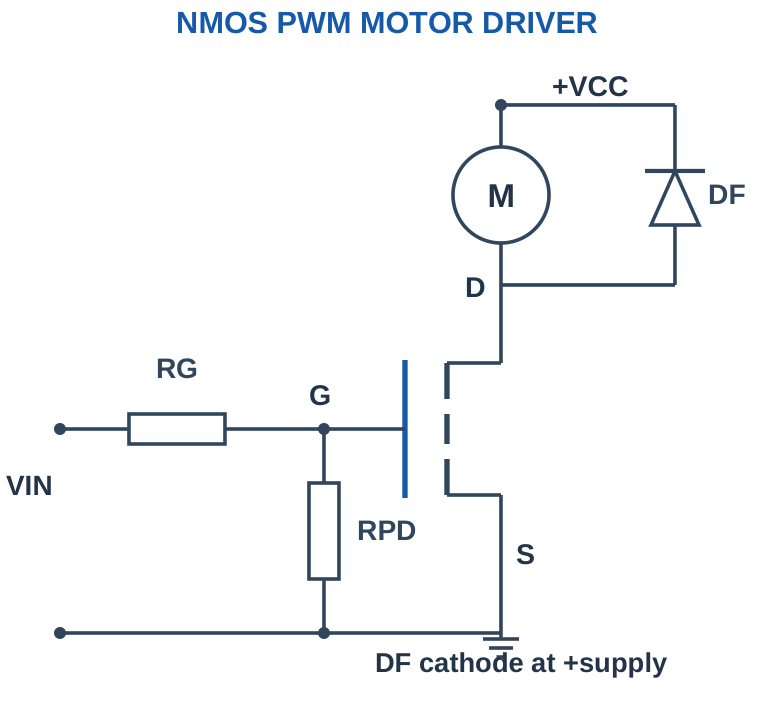
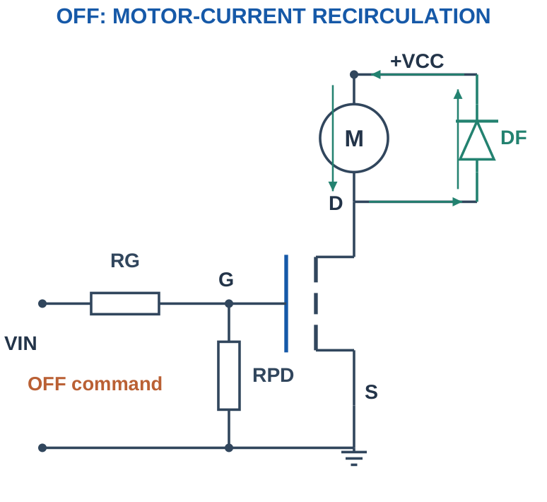
If current is approximately continuous and the MOSFET drop is neglected, average winding terminal voltage can be estimated as DVS – (1 – D)VD for a simple diode-recirculation arrangement with the chosen winding-voltage reference. The ideal zero-drop version is DVS. Current still requires the electrical and mechanical load model.
With a separately supplied approximately constant ON current, MOSFET conduction loss averaged over switching is approximately D I²RDS,on. Use actual current RMS if the current is not adequately represented by this simple assumption. Startup, stall and switching transitions may dominate a real selection.
Worked Problem 2.39: Average Winding Voltage with Recirculation Drop
Problem: For the illustrated low-side motor stage, supply is 12 V, duty 50% and OFF recirculation-diode drop is 0.7 V. Assume continuous current and negligible MOSFET ON drop. Find average winding voltage with the stated polarity.
Model / approach: ON winding voltage is +VS; OFF winding voltage is approximately -VD.
Step 1: Vavg ≈ DVS – (1 – D)VD.
Step 2: Vavg ≈ 0.5 × 12 – 0.5 × 0.7 = 5.65 V.
Answer: Average winding voltage ≈ 5.65 V.
Check and interpretation: This model supplies terminal voltage, not a complete prediction of speed or current. The back EMF, winding resistance and dynamic load must also be compatible with the continuous-current assumption.
PWM QUANTITIES
| Quantity | Expression / Interpretation |
|---|---|
| Period | T = 1/f |
| ON time | ton = DT |
| Resistive RMS | Vrms = VHIGH√D |
| Motor interpretation | Current also depends on inductance and back EMF |
D specifies timing. It is not a universal direct motor-speed fraction.
30. WHY MOSFETS ARE WIDELY USED
MOSFETs suit dense integrated logic because insulated-gate structures can be made small and complementary CMOS logic can have low static conduction in ideal stable states. Dynamic charging, leakage and short-circuit transition currents mean real CMOS power is not zero. Integration and fabrication suitability matter as well as input impedance.
In power switching, appropriate MOSFETs can offer low ON resistance, useful switching speed and drive arrangements that avoid continuous BJT-like base current. However, gate charge, voltage rating, temperature-dependent resistance, switching loss and cost remain trade-offs. A MOSFET is not automatically better in every analog or power application.
Worked check: Same power at different currents
Using supplied constant models, BJT conduction loss is 0.2I and MOSFET loss is 0.05I². They are equal when I = 4 A, giving 0.8 W in either model. This mathematical crossing is not a device recommendation: actual drops, resistance, drive, temperature and ratings must fit the operating conditions.
| Comparison | BJT Switch | MOSFET Switch |
|---|---|---|
| Control quantity in simple model | Base-current drive with appropriate junction voltage. | Gate-to-source voltage and transient charge. |
| ON loss model | VCE,sat IC. | ID²RDS,on. |
| Useful low-loss region name | Saturation. | Ohmic/linear. |
| Critical trap | Using nominal β as guaranteed saturated gain. | Using threshold as guaranteed full enhancement. |
Balanced answer: State the advantage, its operating condition and the trade-off. “MOSFET has no input current and no loss” is not an accurate explanation of its popularity.
31. THREE APPLICATIONS IN ONE VIEW
Home-automation relay: A controller drives a base/gate interface, the transistor energises the coil, and a properly oriented diode gives a recirculation path. The coil circuit and relay-contact circuit are distinct functional parts. Coil current and the available control drive must be compatible.
PWM motor control: A suitable MOSFET repeatedly connects the winding to the supply. Duty cycle changes the applied drive pattern while inductance and back EMF influence current. Motor-current demand, gate drive, recirculation and loss checks are part of the explanation.
Class-A audio voltage amplification: A BJT is biased in active operation, and a small input changes collector current and voltage about Q. Output inversion, coupling and load influence are important. This is different from deliberately saturating the BJT as a relay switch.
Selection checklist for a question: Identify load, supply, intended state, drive capability, voltage/current model and power. This short reasoning order prevents mixing switch and amplifier formulae.
32. [B & C] OPTOCOUPLER: LIGHT ACROSS AN ELECTRICAL BARRIER
An optocoupler transfers information using light between two electrically separated circuits. Its input contains a light emitter, usually an LED. A photosensitive output responds to that light. The input current controls the optical signal; the receiving side supplies its own electrical output energy.
Trace the two loops. On the input side, a resistor sets the emitter current. On the output side, a separately supplied receiver circuit converts the light response into a usable voltage or current. There is no intended metallic signal connection across the optical barrier. Joining the two returns directly can defeat the intended galvanic separation.
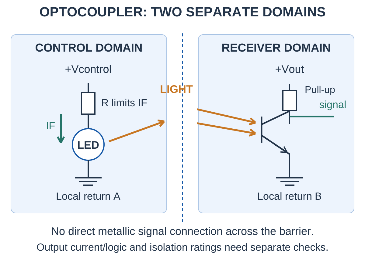
Phototransistor output example. Connect a pull-up resistor on the receiver side to obtain a voltage signal. With sufficient light, the output transistor can pull the node low. Without the input drive, the pull-up tends to take the node high. This commonly inverts the logic; the actual interface must be read from its circuit.
Current transfer ratio. For a specified phototransistor optocoupler operating condition, CTR = IC/IF × 100%. A minimum specified or explicitly supplied CTR is used to check available output current. CTR varies with current, temperature, device spread and ageing. A typical value is not automatically a guaranteed minimum.
Output loading. Compare the receiver current capability with the pull-up and receiving-input demand. Check output voltage, leakage and the stated low-level requirement. An optocoupler does not automatically provide the current needed by a relay coil, solenoid or power-switch gate.
Timing and limits. Phototransistor storage can slow turn-off, especially after deep saturation. For fast switching, use a device and output arrangement suited to the required speed. Propagation delay, rise/fall time and isolation ratings describe different properties.
Isolation boundary. Identify every path crossing between the two domains, including power, signal returns and other cables. A signal optocoupler cannot establish complete system isolation if another connection bridges the same boundary.
Worked Problem 2.40: Optocoupler Input Resistor
Problem: A 5 V control source drives an optocoupler LED with supplied forward drop 1.2 V. Set IF = 10 mA. Find the ideal series resistance and its dissipation.
Model / approach: Use the stated constant-drop LED model.
Step 1: VR = 5 – 1.2 = 3.8 V.
Step 2: R = 3.8/0.010 = 380 Ω.
Step 3: PR = 0.010² × 380 = 0.038 W.
Answer: 380 Ω; resistor dissipation 38 mW.
Check: Recheck current and power after choosing an actual resistor; tolerance and rating margins are additional requirements.
Worked Problem 2.41: Minimum CTR Current Budget
Problem: The supplied minimum CTR is 50% at IF = 8 mA under the stated conditions. Estimate the maximum collector current supported by that minimum-ratio model.
Model / approach: Use IC = (CTR/100)IF.
Step 1: IC = 0.50 × 8 mA = 4 mA.
Answer: 4 mA at the stated ratio and test conditions.
Check: The load circuit must permit that current. A ratio calculation alone does not establish a required saturated output voltage.
Worked Problem 2.42: Receiver Pull-Up Demand
Problem: A receiver node has a 5 V pull-up and a stated desired low voltage 0.2 V. Available sink current at that low voltage is explicitly specified as 2 mA. Find the minimum pull-up resistance that does not demand more current.
Model / approach: Use the supplied low-state capability, not an unqualified typical CTR.
Step 1: Voltage across the pull-up is 5 – 0.2 = 4.8 V.
Step 2: Rmin = 4.8/0.002 = 2400 Ω.
Answer: R must be at least 2.4 kΩ for this current-demand check.
Check: The HIGH-state input leakage and timing impose separate checks; an arbitrarily large resistor is not automatically suitable.
33. [B] INDUSTRIAL RELAY DRIVER: CONTROL AND CONTACTS
A controller output is a signal source with a current limit. A relay coil is a separate load with its own voltage and current requirement. A transistor driver lets the controller command the coil while the load supply provides the coil energy. The relay contacts then operate a separate external circuit.
Read the drawing in layers. First identify the controller-to-base loop. Next trace coil current from the positive coil supply through the coil and conducting transistor to return. Finally identify the contact circuit. A normally open contact is open in the stated de-energised condition; energising the coil changes the contact state.
Industrial interpretation. A relay contact rating applies to a stated load type and switching condition. Coil current is not contact current. Contact isolation and an optocoupler isolation barrier are distinct parts of a system; drawing a relay symbol does not specify every insulation or interface requirement.
Use the shared circuit principles: verify base/gate drive, load current and the stated ON/OFF model. In a DC relay driver, check the flyback path separately from the contact/load circuit.
Worked Problem 2.43: Industrial Relay Base-Drive Selection
Problem: A 24 V relay coil has 600 Ω resistance. Use VCE,sat = 0.2 V, forced beta 10, a 3.3 V drive and VBE = 0.8 V. Find coil current and the maximum ideal base resistance. Check a selected 620 Ω resistor.
Model / approach: Assume the stated ON-switch model, then check available base drive.
Step 1: IC = (24 – 0.2)/600 = 39.6667 mA.
Step 2: IB,required = IC/10 = 3.9667 mA.
Step 3: RB,max = (3.3 – 0.8)/0.00396667 = 630.2521 Ω.
Step 4: At 620 Ω, IB = 2.5/620 = 4.0323 mA.
Answer: 620 Ω supplies enough base current under the stated nominal model.
Check: The control output must be able to deliver this current. Minimum drive voltage, resistor tolerance and device-drop limits still need checking.
34. [B] MOSFET GATE DRIVE IN A VFD: FUNCTIONAL VIEW
A variable-frequency drive changes the electrical excitation supplied to an AC motor. At the functional level, an input rectifier supplies a DC link and an inverter switches that link to produce controlled motor-terminal waveforms. The inverter switching devices require suitable gate-drive circuits.
Where the MOSFET idea fits. A gate driver uses transistor stages to source and sink charge at a power-device gate. A MOSFET may be used in the driver or as a suitable power switch, depending on the design. A VFD need not use MOSFETs as every inverter power device; many implementations use IGBTs or other devices.
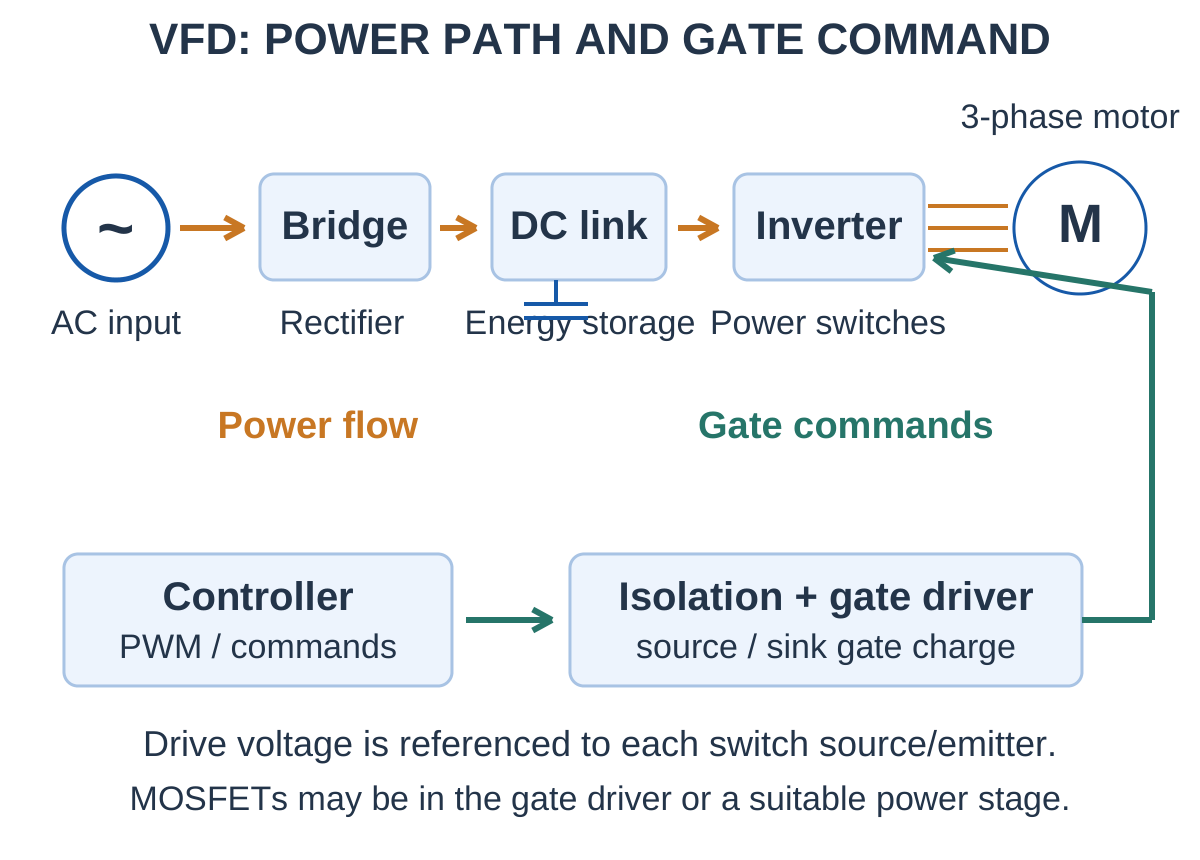
Reference matters. A low-side source may be near the power return. A high-side source or emitter moves with the switching node. Its gate drive must therefore be established relative to its own source/emitter, not judged only against the controller ground. This is the same VGS subtraction principle used in the basic NMOS examples.
Charge and discharge. The driver must rapidly move gate charge to create controlled transitions. Small average gate current can coexist with a much larger transition current. The optocoupler or digital isolator transfers a command; a separate drive stage may be needed to deliver the required gate current.
Complementary switches. The two devices of an inverter leg must not form an unintended direct conducting path across the DC link. Gate-drive timing, interlocks and dead time are used in the functional explanation. Dead time must be coordinated with actual delays and turn-off behaviour.
Scope of the model. The introductory diagram identifies rectifier, DC link, controller, isolation/driver and inverter. It is not a complete VFD design. Device ratings, layout, current sensing and protection influence a practical implementation.
Worked Problem 2.44: Gate-Driver Transition Current
Problem: A supplied gate-charge interval is 40 nC and should be moved in 200 ns. Estimate the constant current required during that interval.
Model / approach: Use I = Q/t for the explicitly idealised interval.
Step 1: I = 40 × 10^-9/(200 × 10^-9) = 0.2 A.
Answer: 200 mA during the idealised charging interval.
Check: This is a transition current, not the average gate current over the entire switching cycle.
35. [B] PLC OUTPUT ISOLATION AND LOAD INTERFACING
Draw two supplies when required. The controller-side return and load-side return belong to different domains in an isolated diagram. Do not connect them with an unlabelled ground line. A common reference is appropriate in a non-isolated driver but contradicts the intended galvanic separation of a simple isolated signal path.
Check both sides. On the input, verify LED current, input voltage and resistor power. On the receiver, verify minimum CTR or a specified logic-output capability, pull-up demand, low/high thresholds and response time. On the load driver, verify drive current, load path and inductive recirculation.
Logic state. A phototransistor pull-up arrangement often makes LED ON correspond to output LOW. Decide whether the next stage interprets that as an asserted or deasserted command. Keep physical current flow separate from the words ON, HIGH and active-low.
Fault reasoning. A valid PLC command does not prove that the receiving supply is present. Check the input LED drive, output-side supply, local signal, transistor drive and load current in sequence. Each measurement should test one stage rather than assign every failure to the optocoupler.
Use the shared circuit principles: verify base/gate drive, load current and the stated ON/OFF model. In a DC relay driver, check the flyback path separately from the contact/load circuit.
36. [B] SOLID-STATE RELAY: ELECTRONIC LOAD CONTROL
A solid-state relay (SSR) uses an electronic input interface and semiconductor output switching rather than a mechanically moving contact. Some SSRs use optical coupling for input-output isolation. The output device and circuit determine whether a particular SSR is suitable for AC, DC or a specified load condition.
Input. The control side must provide the stated input voltage/current range. A packaged input may include a limiting network; a bare optocoupler LED does not. Read the specified input arrangement instead of assuming every SSR input is directly interchangeable with a transistor base.
Output. AC SSRs may use a triac or thyristor arrangement that turns off when load current falls below its holding condition. A DC MOSFET-output SSR has different switching behaviour. A triac-output AC SSR is not a general DC switch.
Zero-cross concept. Some AC SSRs delay turn-on until near a voltage zero crossing to reduce certain switching disturbances. This is different from arbitrary phase-angle control. The meaning of turn-off depends on the output device and load current, not just the input command.
Losses and leakage. An SSR can have a nonzero ON drop or ON resistance, creating heat under load. It can also pass OFF-state leakage current. An electronic OFF indication is therefore not equivalent to a mechanically open air gap with zero leakage in every application.
Compare with an electromechanical relay. An SSR has no moving output contact and can suit frequent switching. A mechanical relay provides contact behaviour with wear and finite mechanical operating time. Compare load type, leakage, voltage drop, heat, switching rate and isolation specification for the stated task.
Worked Problem 2.45: SSR ON-Drop Heating
Problem: A stated SSR model has a constant 1.2 V ON drop while carrying 3 A continuously. Estimate output-stage conduction loss.
Model / approach: Use P = VON I.
Step 1: P = 1.2 × 3 = 3.6 W.
Answer: 3.6 W under the supplied constant-drop model.
Check: Thermal conditions and rating limits decide whether that dissipation is acceptable.
Worked Problem 2.46: OFF Leakage Through a Resistive Load
Problem: A specified OFF leakage of 0.5 mA flows through a 10 kΩ resistor. Under this stated current model, calculate the resistor voltage.
Model / approach: Apply Ohm’s law to the given leakage current.
Step 1: V = 0.0005 × 10000 = 5 V.
Answer: 5 V across the stated resistor.
Check: The source and complete leakage model must support this condition. OFF-state leakage can produce a measurable load voltage.
37. [C] DRIP-IRRIGATION SOLENOID VALVE CONTROL
A solenoid valve converts electrical coil energisation into a mechanical change in the valve. In a relay-driven irrigation arrangement, the controller drives a transistor, the transistor energises a relay coil and the relay contacts switch the valve supply. The relay coil and valve coil are separate loads.
Functional chain. A moisture reading or schedule produces a command. A suitable driver energises the relay coil. The contact state applies or removes power to the valve. A normally closed valve description refers to the valve state without its operating power; a normally open relay contact refers to a contact state. Do not confuse these labels.
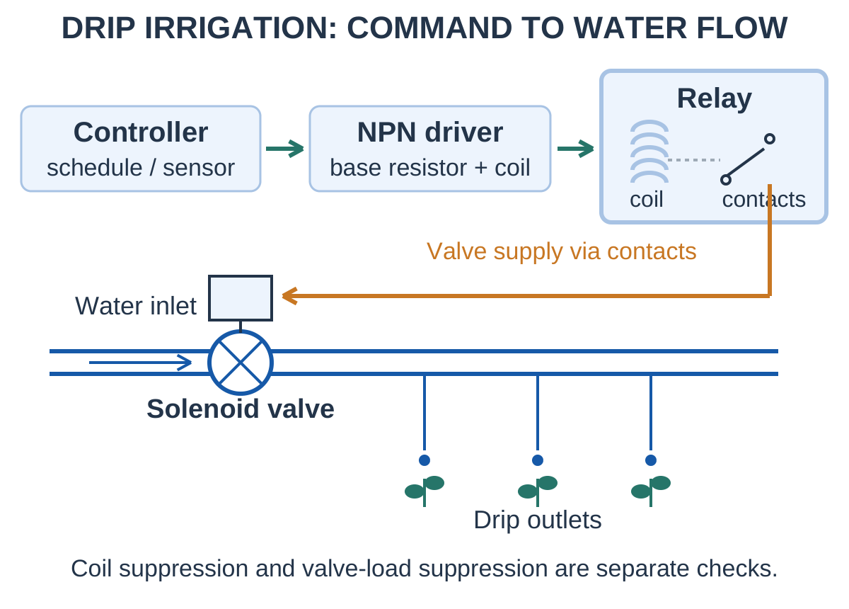
Inductive turn-off. A DC relay coil needs an appropriate current-recirculation arrangement. A DC solenoid valve may also need its own suppression at its own switched circuit. A diode across the relay coil does not automatically clamp a separate valve coil switched by the contacts.
Valve supply. Some valves operate from AC and others from DC. Apply the suppression method appropriate to the specified supply and load; the simple DC flyback diode diagram must not be transferred unchanged across an AC coil. The notes use explicitly stated DC examples.
System checks. Verify valve voltage, current, contact capability, controller drive and the chosen default state. A lit indicator or audible relay click does not establish water flow. Electrical command, mechanical valve motion and hydraulic flow are separate observations.
Worked Problem 2.47: Energy in a DC Valve Coil
Problem: A supplied coil model has L = 0.2 H and carries 0.5 A immediately before turn-off. Find stored magnetic energy.
Model / approach: Use E = LI²/2.
Step 1: E = 0.5 × 0.2 × 0.5² = 0.025 J.
Answer: 25 mJ of stored magnetic energy.
Check: Energy must be redistributed during turn-off; this calculation alone does not select a suppression device.
38. [C] BIOMEDICAL BUZZER OR ALARM DRIVER
A diagnostic or monitoring device may use an audible alarm to communicate a selected condition. A transistor switch lets a low-current logic output command a buzzer supplied from a suitable rail. The trigger decision belongs to the instrument processing; the transistor implements the electrical output action.
Load type. A magnetic sounder can involve inductance, whereas a piezo element has a different electrical model. Choose suppression or a drive waveform for the actual component. Do not add a relay-coil flyback diode blindly to every piezo circuit without identifying the load.
Default state and diagnosis. A pull-down or suitable bias network can give a defined OFF state when the control output is inactive. To investigate a silent alarm, check supply, command, drive current, transistor state and load continuity. A normal logic voltage does not establish enough base current.
Meaning of the indicator. The audible output reports the state requested by the system. This unit explains the switch and interface; it does not infer a medical condition from the sounder circuit or establish the reliability of the complete alarm system.
Worked Problem 2.48: Alarm-Switch Conduction Loss
Problem: An active buzzer draws 50 mA and the saturated transistor drop is supplied as 0.2 V. Find transistor collector-path conduction loss while ON.
Model / approach: Use P = VCE,sat IC.
Step 1: P = 0.2 × 0.050 = 0.010 W.
Answer: 10 mW in the stated collector-path model.
Check: Base-drive dissipation is separate. The buzzer power and transistor power are different quantities.
39. [C] MOSFET SWITCH IN A SOLAR CHARGE CONTROLLER
A solar charge controller manages energy transfer between a photovoltaic source, a storage battery and sometimes a load. A MOSFET can act as a controlled switching element in that power path. The sensing, control algorithm and complete power-converter topology determine how charging is managed.
Functional chain. Voltage/current sensing informs a control stage. A gate driver applies an appropriate gate-to-source voltage to the MOSFET. Switching changes the conducting energy path. The supply or panel provides power; the gate command controls it and does not supply the charging current itself.
OFF is directional. The intrinsic body diode can permit current in one direction even when the gate is OFF. A single MOSFET is not automatically a bidirectional blocking switch. Reverse-current control depends on the actual device arrangement and topology.
Limits of a simple switch. A diode, MOSFET and a PWM command alone do not specify a complete battery charging method. The controller must implement the charging requirements of its battery and power circuit. Here the purpose is to explain the MOSFET switching role and elementary drive/loss calculations.
Worked Problem 2.49: Solar-Switch ON Loss
Problem: A switch carries a constant 4 A with supplied RDS,on = 0.025 Ω at the stated drive and temperature. Find drop and loss.
Model / approach: Use the adequately enhanced resistive ON model.
Step 1: VDS = 4 × 0.025 = 0.1 V.
Step 2: P = 4² × 0.025 = 0.4 W.
Answer: 0.1 V drop and 0.4 W conduction loss.
Check: These values apply to the supplied operating conditions, not every gate voltage or temperature.
Worked Problem 2.50: Duty-Weighted Solar-Switch Loss
Problem: An idealised switch carries 8 A during an ON fraction D = 0.6 and zero during the rest of the period. Its supplied ON resistance is 0.04 Ω. Find IRMS and average channel conduction loss.
Model / approach: Use the specified rectangular switch-current waveform.
Step 1: IRMS = 8√0.6 = 6.1968 A.
Step 2: Pcond = D ION² R = 0.6 × 64 × 0.04 = 1.536 W.
Answer: IRMS ≈ 6.1968 A; conduction loss 1.536 W.
Check: The waveform is explicitly supplied. Do not infer this current shape for every solar converter; switching losses are omitted.
40. [C] OPTOCOUPLER IN ECG ISOLATION: PATIENT-SAFETY CONCEPT
An ECG measurement chain receives small electrode-related signals and processes them for display or further analysis. A conceptual isolation barrier separates the patient-connected acquisition domain from another electrical domain. Information can cross a barrier optically while there is no intended direct metallic signal path.
Separate the domains. Show patient-connected electrodes and acquisition electronics on one side, and a receiving/processing interface on the other. Mark the barrier. Include the power arrangement in the explanation: a signal barrier alone does not remove an unintended connection through a shared supply or another cable.
Optocoupler role. An emitter on one side sends light to a receiver on the other. The optical signal represents information. Each side requires its own compatible electrical circuitry. The receiving electronics provide their own local output energy.
Preserving information. A basic phototransistor optocoupler is not automatically a precise linear analog ECG channel. CTR varies, and nonlinearity, bandwidth and noise affect the transferred signal. Depending on the architecture, information may be encoded/digitised before isolation or transferred through a suitable linear isolation stage.
What the drawing proves. A functional optocoupler diagram explains galvanic signal separation. It does not prove patient protection by itself. Complete medical isolation also depends on rated barriers, isolated power where required, leakage control, insulation and the applicable system design requirements.
Exam answer. State the purpose of the barrier, show separated reference domains, explain emitter-to-receiver transfer and acknowledge the need to preserve the measurement information. Do not connect an unlabelled common ground across the barrier or label an ordinary optocoupler alone as a complete patient-protection system.
41. DIAGNOSIS AND COMMON MISTAKES
A load that does not turn on can have insufficient drive, incorrect pin identification, an unsuitable model, an open connection or a load/supply problem. A single symptom does not uniquely identify a failed transistor. Start by comparing the expected terminal voltages and current paths with observations.
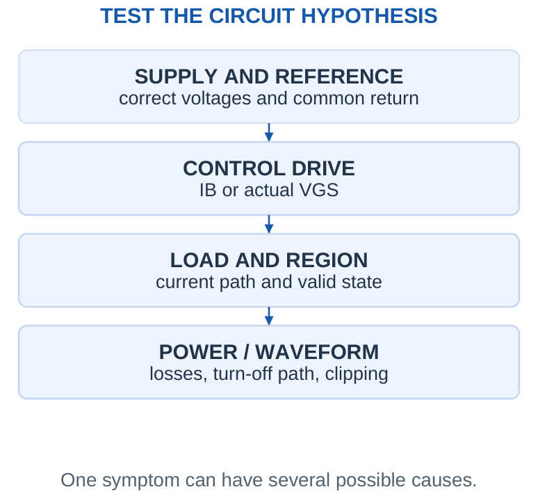
| Observation | Useful Check |
|---|---|
| BJT collector not low when commanded ON | Base current, available load current and the saturation assumption. |
| MOSFET heats despite a positive gate voltage | Actual VGS, relevant RDS,on, current and switching conditions. |
| Motor causes turn-off voltage stress | Recirculation path and diode orientation. |
| CE output clipped | Q point, input amplitude, load and available swing. |
| Buzzer only clicks | Whether the transducer needs a varying excitation. |
Error-correction habit: Use the relevant physical quantity: VBE for BJT input, VGS for MOSFET drive, load current for ON demand and power for heating. One voltage reading does not substitute for every check.
Worked check: A useful fault question
A MOSFET gate measures 5 V to ground while its source measures 4 V. The immediate useful calculation is VGS = 1 V. Replacing the device without checking that difference would skip a possible drive problem. A terminal measurement should test the actual hypothesis rather than rely on the word HIGH at a controller output.
42. FORMULAE AND EXAM TRICKS
Fast checks: Add BJT terminal currents before calculating gain. Test collector voltage after βIB. Count voltage drops in the actual load path. Use a stated forced beta for switch-drive sizing. For MOSFETs, subtract source voltage before judging drive. Do not call threshold a full-ON rating. Use RMS for resistive heating and peak swing for clipping. Check flyback-diode cathode toward positive supply in the illustrated low-side circuits.
| Quantity | Expression and Condition |
|---|---|
| BJT current | IE = IC + IB; consistent current magnitudes |
| Forward-active gain | IC = βIB; verify the collector circuit |
| Switch load current | IC ≈ (VCC – VCE,sat)/RL |
| Required base drive | IB ≥ IC/βforced; supplied design model |
| Base resistor | RB = (Vdrive – VBE)/IB |
| Coil energy | E = LI²/2 |
| Gate-to-source voltage | VGS = VG – VS |
| MOSFET conduction loss | P = IRMS²RDS,on at stated conditions |
| Gate-charge interval | t ≈ Qg/Idrive; supplied interval model |
| PWM duty and timing | D = ton/T; f = 1/T |
| Rectangular resistive PWM | Vavg = DVS; Vrms = VS√D |
| CE voltage gain | Av = vo,ac/vi,ac; sign indicates inversion |
| Sinusoidal signal power | Psignal = Vrms²/RL |
| Simple class-A input | PDC = VCC ICQ under stated boundary |
| Current transfer ratio | CTR = IC/IF × 100%; stated conditions |
| Optical-input resistor | R = (Vdrive – VF)/IF |
| Receiver pull-up demand | I = (Vpullup – Vlow)/Rpullup |
Formula rule: A neat calculation is not sufficient: the model, waveform, region and load conditions must be valid. Use the supplied parameter at its stated operating point.
FINAL MODEL COMPARISON
| Task | Required Reasoning |
|---|---|
| BJT switch | Load-limited ON current + adequate base drive |
| MOSFET switch | VGS, ON resistance, transient charge and loss |
| Application | Trace command, energy path and practical limits |
Write the model and assumptions before selecting an equation.
43. QUICK REVISION: EXPLAIN AND CHECK
Why Can IC = βIB Fail in a Switch?
The external collector circuit may not support the predicted current. Recalculate with the stated saturation model and check that the available base drive is sufficient.
What Does a Flyback Diode Do?
It provides a continuing current path for a DC inductive load at turn-off. In the low-side example its cathode is at the positive coil supply.
Why Is a Gate Voltage to Ground Insufficient?
MOSFET drive depends on VG – VS. A moving source changes VGS even when the gate-to-ground voltage remains unchanged.
Is Threshold a Guaranteed Full-ON Drive?
No. Threshold is specified at a small current. Use the stated ON resistance or appropriate operating data at the intended gate drive.
Does a MOSFET Driver Supply No Current?
Steady leakage may be small, but transitions require gate charge to be supplied and removed.
How Is Power Checked?
Use the relevant ON drop or resistance, the appropriate current waveform and the stated thermal model. Separate conduction, switching and drive losses.
Why Does a CE Stage Invert Voltage?
An input increase can increase collector current, increasing the RC drop and lowering collector voltage while the device remains in active operation.
What Makes a Stage Class A?
The device conducts throughout the intended signal cycle about a suitable bias point. Signal power comes from the supply.
Does Duty Cycle Directly Equal Motor-Speed Fraction?
No. It specifies drive timing; speed also depends on load, back EMF, supply and the control system.
What Does an Optocoupler Transfer?
Information crosses as light between separate electrical domains. The output circuit uses its own supply.
Why Distinguish a Relay Coil from Valve Current?
The transistor may energise the relay coil while the contacts switch a separate valve supply and load.
Does an Optocoupler Alone Prove ECG Patient Protection?
No. Signal integrity, rated barriers, power isolation where required and complete system design must also be considered.
Can Every SSR Switch DC?
No. A triac-output AC SSR depends on current commutation; select a suitable output type for the stated load.
What Does a VFD Gate Driver Supply?
It supplies and removes gate charge at the required source/emitter reference. It is distinct from the motor-power path.
Does an OFF MOSFET Always Block Reverse Current?
No. The intrinsic body diode can conduct in one direction. Blocking depends on the actual topology.
Why Distinguish Active and Passive Buzzers?
An active buzzer contains an oscillator. A passive element requires a suitable changing excitation for a sustained tone.
Final Check
Label terminals → trace paths → choose model → calculate → verify region, ratings and physical meaning.
| Task | Intended Operation | Essential Check |
|---|---|---|
| BJT switch | Cut-off / saturation | Load current and adequate base drive |
| CE amplifier | Forward active about Q | Gain, loading and signal headroom |
| NMOS switch | Adequately driven ohmic ON state | VGS, current waveform and loss |
| Optical interface | Separate electrical domains | Signal transfer, loading and complete barrier |