University: Dr. A.P.J. Abdul Kalam Technical University, AKTU
Programme: B.Tech First Year, Semester I and Semester II
Course Codes: AEE101A / AEE201A
Branches: Common to All
Unit: II
Unit Name: AC Circuits
Introduction to AC Circuits
Alternating-current circuit analysis explains electrical quantities that change continuously with time. Unlike the constant quantities used in elementary steady DC circuits, an alternating voltage reverses its polarity periodically, while an alternating current reverses its direction.
The sinusoidal waveform is the main model used in this unit. Its behaviour can be described through amplitude, frequency and phase. These three properties must be distinguished because two waveforms can have the same frequency while differing in amplitude or timing.
A resistor, an inductor and a capacitor respond differently to the same sinusoidal voltage. In an ideal resistor, voltage and current are in phase. In an ideal inductor, current lags voltage. In an ideal capacitor, current leads voltage. These phase relationships determine impedance, power factor and the direction of reactive-power exchange.
Phasors provide a convenient way to retain both magnitude and phase without repeatedly writing complete time-domain equations. Complex numbers allow the same circuit laws used in DC analysis to be applied to sinusoidal steady-state circuits.
Power in an AC circuit also requires careful interpretation. The product of RMS voltage and RMS current gives apparent power. Average active power additionally depends on phase displacement. Reactive power describes the alternating exchange associated with ideal magnetic and electric energy storage.
The unit connects waveform generation with RMS values, phasor operations, pure R, L and C circuits, series RL and RC networks, power-factor correction and single-phase wattmeter measurement.
Unit 2 Topic Map
| Topic | Main Coverage |
|---|---|
| AC generation | Rotating coil, flux linkage and sinusoidal EMF |
| Waveform timing | Period, frequency and angular frequency |
| Waveform values | Instantaneous, peak, RMS and average values |
| Waveform factors | Form factor and crest factor |
| Phasors | RMS magnitude, phase and common references |
| Complex representation | Rectangular and polar forms |
| Phasor addition | Equal-frequency voltage and current combinations |
| Pure resistor | In-phase current and active power |
| Pure inductor | Lagging current and magnetic energy |
| Pure capacitor | Leading current and electric energy |
| Series RL circuits | Impedance, voltage triangle and coil identification |
| Series RC circuits | Impedance, voltage triangle and capacitance calculation |
| Frequency dependence | Changes in reactance, current and power factor |
| AC power | Active, reactive, apparent and complex power |
| Combined loads | Addition of active and reactive powers |
| Power-factor correction | Shunt capacitor and source-current reduction |
| Measurement | Wattmeter connections, readings and range checks |
Syllabus Coverage
- Generation of alternating voltage.
- Sinusoidal waveform parameters.
- Peak, RMS and average values.
- Form factor and crest factor.
- Simple phasor representation.
- Rectangular and polar complex forms.
- AC through pure resistance.
- AC through pure inductance.
- AC through pure capacitance.
- Series RL and RC circuits.
- Impedance and phase relationships.
- Active, reactive and apparent power.
- Power factor and its improvement.
- Single-phase shunt capacitor calculations.
- Single-phase wattmeter measurement.
- Numerical verification and examination practice.
Conventions Used Throughout the Article
Unsubscripted V and I represent RMS values unless another meaning is explicitly stated. Vm and Im represent peak values.
All phasors in a single calculation use the same frequency and the same time reference. These notes use a common sine convention for converting between phasors and time equations.
The phase angle φ is defined as:
φ = Voltage phase − Current phase
A positive φ represents lagging current and inductive behaviour. A negative φ represents leading current and capacitive behaviour.
Inductive reactive power is positive. Capacitive reactive power is negative. Apparent-power magnitude is non-negative.
Components and instruments are ideal unless resistance, losses, loading or another practical effect is supplied in the problem.
Retain useful precision during calculations. Round the final numerical result and include the correct unit and phase direction.
1. Generation of Alternating Voltage
An alternating voltage changes polarity periodically. A sinusoidal alternating voltage follows a sine law and provides the standard waveform model for the calculations in this unit.
One complete cycle contains a positive half-cycle and a negative half-cycle. The sign identifies instantaneous polarity relative to a selected pair of terminals.
A sinusoidal voltage can be generated when the magnetic flux linkage of a coil changes sinusoidally. A rotating coil in a uniform magnetic field provides a simple model.

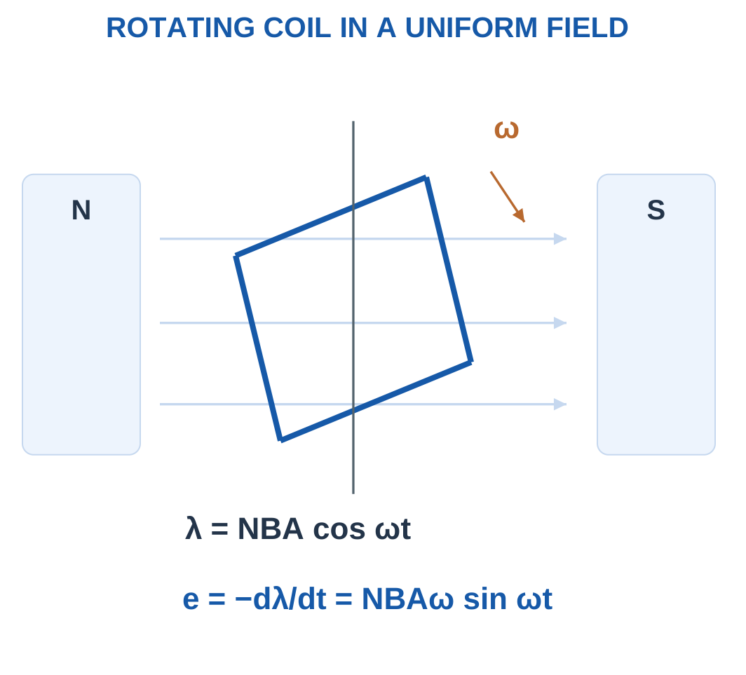
Consider a coil having:
- N turns.
- Area A per turn.
- Uniform magnetic flux density B.
- Angular speed ω.
- Angle θ between the magnetic field and the coil’s normal.
Flux through one turn is:
Φ = BA cos θ
For uniform rotation with the stated initial position:
θ = ωt
Flux linkage is therefore:
λ = NBA cos ωt
Faraday’s law gives:
e = −dλ/dt
Differentiating:
e = NBAω sin ωt
The peak induced EMF is:
Em = NBAω
Therefore:
e = Em sin ωt
If peak flux per turn Φm is already supplied, use:
Em = NωΦm
Do not multiply by coil area again when Φm already includes the magnetic field and area.
Relationship Between Flux and EMF
The induced EMF depends on the rate of change of flux linkage rather than simply its magnitude.
At maximum positive or negative flux linkage, the instantaneous rate of change is zero, so induced EMF is zero.
When flux linkage passes through zero most rapidly, the magnitude of induced EMF is greatest.
This explains the quarter-cycle displacement between the cosine flux-linkage waveform and the sine EMF waveform in the selected reference.
The elementary model gives one electrical cycle per mechanical revolution. More complicated pole arrangements belong to machine analysis and are not required for these examples.
Worked Problem 2.1: Coil EMF from Field and Area
Problem: A 100-turn coil of area 0.01 m² rotates at 50 cycles per second in a uniform 0.4 T field. Find peak flux per turn, peak EMF and RMS EMF.
Step 1: Calculate peak flux per turn.
Φm = BA.
Φm = 0.4 × 0.01.
Φm = 0.004 Wb.
Step 2: Calculate angular frequency.
ω = 2πf = 2π × 50.
ω = 314.159 rad/s.
Step 3: Calculate peak EMF.
Em = NωΦm.
Em = 100 × 314.159 × 0.004.
Em = 125.664 V.
Step 4: Convert to RMS.
E = Em/√2.
E ≈ 88.8577 V RMS.
The signed average over a complete cycle is zero even though RMS voltage is nonzero.
Worked Problem 2.2: Increasing Coil Turns
Problem: A 200-turn coil of area 0.015 m² rotates at 25 cycles per second in a 0.25 T field.
Peak flux:
Φm = 0.25 × 0.015.
Φm = 0.00375 Wb.
Angular frequency:
ω = 2π × 25.
ω = 157.08 rad/s.
Peak EMF:
Em = 200 × 0.00375 × 157.08.
Em = 117.81 V.
RMS EMF:
E = 117.81/√2.
E ≈ 83.3041 V RMS.
The result depends on turns, flux per turn and speed together. Increasing turns alone increases EMF, but the other parameters in this example differ from the previous example.
Worked Problem 2.3: Peak Flux and RMS EMF
Problem: An 80-turn coil of area 0.02 m² rotates at 60 cycles per second in a uniform 0.6 T field.
Φm = BA = 0.6 × 0.02.
Φm = 0.012 Wb.
ω = 2π × 60.
ω = 376.991 rad/s.
Em = 80 × 0.012 × 376.991.
Em ≈ 361.911 V.
E = Em/√2.
E ≈ 255.91 V RMS.
The flux linkage is maximum at the selected zero-time position, while the induced EMF is zero at that same instant because the derivative of flux linkage is zero.
2. Time Period, Frequency and Angular Frequency
The time period T is the time required for one complete repetition of a waveform.
Frequency f is the number of complete cycles occurring each second.
f = 1/T
T = 1/f
The unit hertz means cycles per second.
Angular frequency measures the rate of phase-angle change:
ω = 2πf
Its unit is radians per second.
One complete cycle corresponds to:
360° = 2π radians

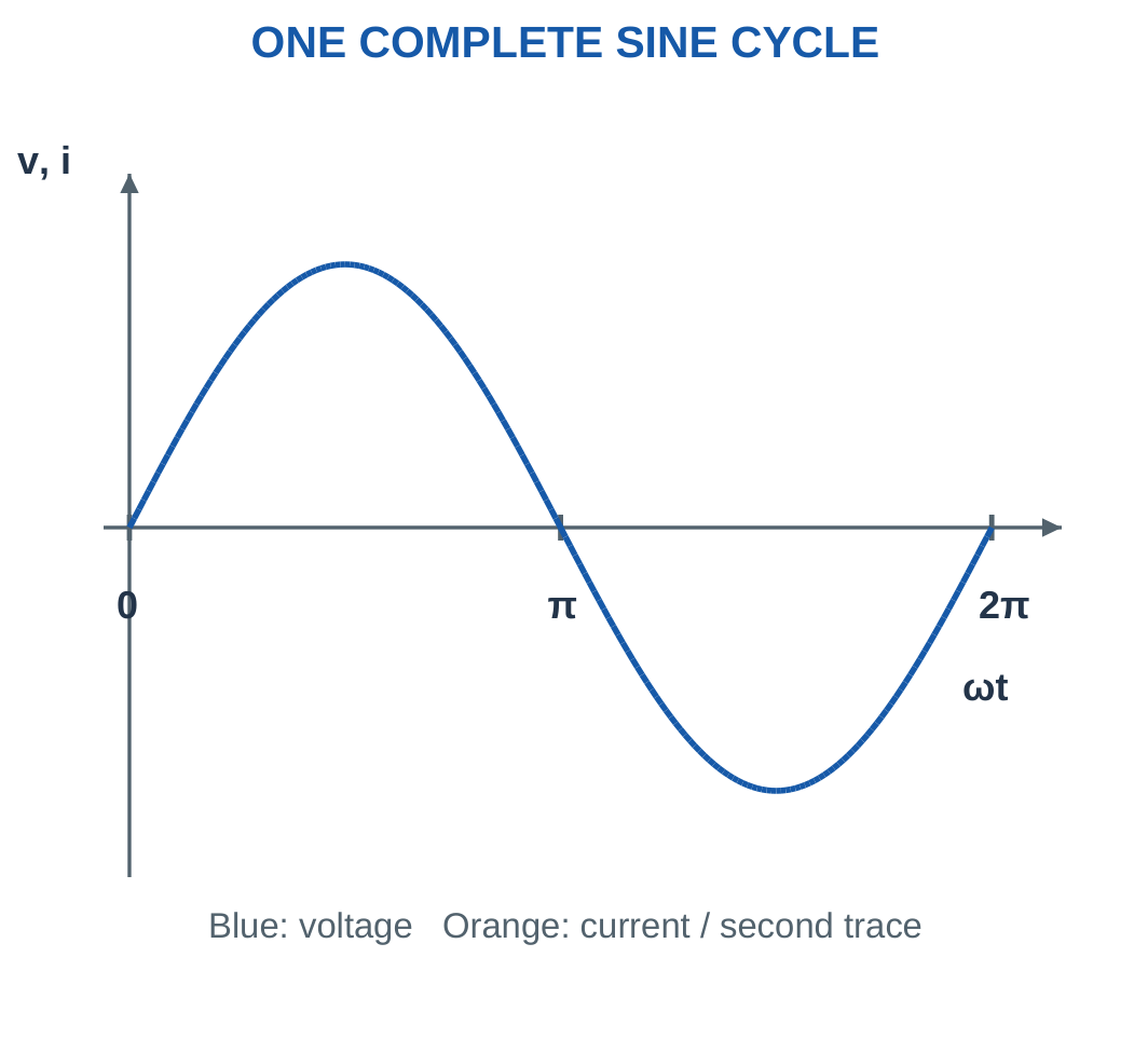
For the waveform:
v(t) = Vm sin(ωt + θ)
Vm determines peak amplitude. Angular frequency determines how quickly the waveform repeats. Initial phase θ determines its position relative to the chosen time reference.
Changing amplitude does not change frequency. Changing phase does not change period. These parameters should be identified separately before calculation.
For an unshifted sine wave:
- The first positive peak occurs at T/4.
- The next zero crossing occurs at T/2.
- The first negative peak occurs at 3T/4.
- The next complete cycle begins at T.
Converting Time Delay into Phase
A time interval Δt corresponds to:
Δθ = 360fΔt degrees
or:
Δθ = 2πfΔt radians
The same delay produces a larger phase displacement at a higher frequency.
A delayed sine waveform can be written:
sin[ω(t − Δt)]
Expanding the argument shows a negative initial phase. Therefore a waveform reaching a corresponding point later in time lags the reference.
Convert milliseconds into seconds before using a formula containing frequency in hertz.
Worked Problem 2.4: Reading a Complete Cycle
Problem: A sinusoid has frequency 25 Hz. Find period, angular frequency, first positive-peak time and the separation between opposite peaks.
T = 1/25.
T = 0.04 s = 40 ms.
ω = 2π × 25.
ω = 157.08 rad/s.
First positive peak:
T/4 = 40/4.
Time = 10 ms.
First negative peak:
3T/4 = 30 ms.
Opposite peaks are separated by:
T/2 = 20 ms.
Consecutive positive peaks are separated by a complete period, 40 ms.
Signal Generator and Test Leads


A generated waveform requires amplitude, frequency, offset and reference definitions. A peak specification is not interchangeable with an RMS specification.
Signal-source settings may also depend on the stated termination or load. In a numerical problem, use the waveform and source model explicitly supplied.
Worked Problem 2.5: Timing at 60 Hz
Problem: Repeat the timing calculation for a 60 Hz sinusoid.
T = 1/60.
T = 0.0166667 s = 16.6667 ms.
ω = 2π × 60.
ω = 376.991 rad/s.
First positive peak:
T/4 = 4.16667 ms.
First negative peak:
3T/4 = 12.5 ms.
Separation between opposite peaks:
T/2 = 8.33333 ms.
The frequency value 60 Hz is not the same as an angular frequency of 60 rad/s.
3. Instantaneous Value and Phase Reference
An instantaneous value is the signed value of a waveform at a particular time.
For:
v = 100 sin ωt
the peak remains 100 V, but the instantaneous value can be positive, negative or zero depending on time.
RMS value describes the waveform over an averaging interval. It is not a sample taken at one instant.

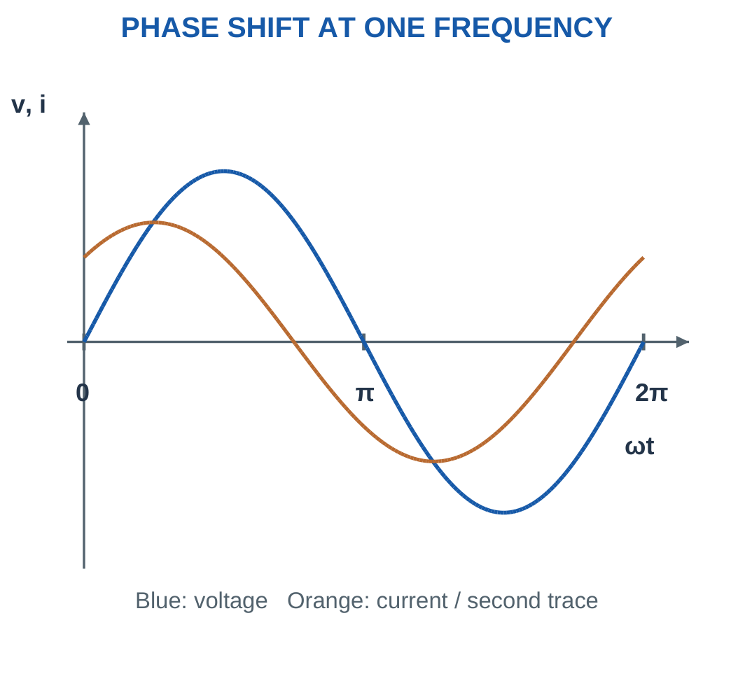
For:
v = Vm sin(ωt + θv)
and:
i = Im sin(ωt + θi)
define:
φ = θv − θi
If φ is positive, current lags voltage. If φ is negative, current leads voltage.
A positive phase in sin(ωt + θ) shifts a corresponding feature toward earlier time. A negative phase shifts it toward later time.
When comparing sine and cosine waveforms, first convert them to a common convention:
cos α = sin(α + 90°)
Do not compare two phase angles written using different waveform conventions without making this conversion.
A fixed phasor diagram also requires a common frequency. Two waveforms with different frequencies do not maintain one constant phase separation.
Oscilloscope Measurement Context


An oscilloscope displays time-varying voltage relative to a defined reference. Probe connection, scale and bandwidth affect interpretation.
The numerical waveform is established by the stated equation or labelled trace. The instrument illustration provides physical context rather than replacing the mathematical signal definition.
Worked Problem 2.6: Delay Converted into Phase
Problem: At 60 Hz, current reaches a corresponding zero crossing 1.5 ms after voltage. Current is 4 A RMS. Find phase displacement and a current time equation.
Δt = 1.5 ms = 0.0015 s.
φ = 360 × 60 × 0.0015.
φ = 32.4° lagging.
Current peak:
Im = √2 × 4.
Im = 5.65685 A.
Angular frequency:
ω = 376.991 rad/s.
Convert phase to radians:
32.4° = 0.565487 rad.
With voltage as the unshifted sine reference:
i = 5.65685 sin(376.991t − 0.565487) A
The negative current phase represents its delay relative to voltage.
Worked Problem 2.7: Delay at 25 Hz
Problem: At 25 Hz, current reaches its corresponding zero crossing 5 ms after voltage. Current is 4 A RMS.
Δt = 0.005 s.
φ = 360 × 25 × 0.005.
φ = 45° lagging.
ω = 157.08 rad/s.
Im = 5.65685 A.
Using radians consistently:
i = 5.65685 sin(157.08t − 0.785398) A
The same delay formula can be evaluated using Δt/T. Here 5 ms is one eighth of the 40 ms period, corresponding to 45°.
Worked Problem 2.8: Instantaneous Voltage
Problem: For v = 200 sin(2π × 50t) V, calculate voltage at 2 ms and identify RMS voltage.
t = 0.002 s.
Time angle:
2πft = 2π × 50 × 0.002.
Angle = 0.628319 rad = 36°.
v = 200 sin 36°.
v ≈ 117.557 V.
RMS voltage:
V = 200/√2.
V ≈ 141.421 V.
The RMS value comes from peak amplitude, not from dividing the instantaneous 117.557 V sample by √2.
Worked Problem 2.9: Include Initial Phase
Problem: For v = 325 sin(2π × 50t + 30°) V, find voltage at 5 ms.
The time angle at 5 ms is 90°.
Total angle:
90° + 30° = 120°.
v = 325 sin 120°.
v ≈ 281.458 V.
RMS voltage:
V = 325/√2.
V ≈ 229.81 V.
When entering the equation in a calculator, either evaluate all angles in degrees or convert the initial phase to radians before adding it to ωt.
Worked Problem 2.10: A Negative Initial Phase
Problem: For v = 100 sin(2π × 25t − 30°) V, find voltage at 10 ms.
At t = 0.01 s:
Time angle = 2π × 25 × 0.01.
Time angle = 90°.
Total angle:
90° − 30° = 60°.
v = 100 sin 60°.
v ≈ 86.6025 V.
RMS voltage:
V = 70.7107 V.
The negative initial phase delays the waveform but does not change its peak or RMS magnitude.
4. RMS Value and Its Heating Meaning
RMS means root mean square. It is calculated by squaring the instantaneous waveform, finding the mean of the squared values and taking the positive square root.
For voltage over one period:
Vrms = √[(1/T)∫₀ᵀv²dt]
For current:
Irms = √[(1/T)∫₀ᵀi²dt]
Squaring removes the sign of each instantaneous sample. Taking the mean accounts for the complete waveform. Taking the square root restores the original electrical unit.
For a sinusoid:
v = Vm sin ωt.
Therefore:
v² = Vm² sin² ωt.
The full-cycle average of sin² ωt is one half, so:
Vrms = Vm/√2
Similarly:
Irms = Im/√2


Why RMS Is an Effective Value
For an ideal resistor:
p(t) = i²(t)R
Average heating power is:
P = Irms²R
A DC current numerically equal to the AC RMS current produces the same average resistor heating.
This does not mean the instantaneous power waveforms are identical. DC power is constant for constant resistance, while sinusoidal resistor power varies at twice the electrical frequency.
A quoted sinusoidal supply voltage in circuit problems normally means RMS unless peak is stated.
For example, 230 V RMS corresponds to a peak of approximately 325.3 V. Writing 230 sin ωt would describe a 230 V peak waveform, not a 230 V RMS waveform.
The factor 1/√2 applies specifically to a sinusoid. Other wave shapes require the general mean-square definition.
Worked Problem 2.11: RMS Voltage and Equivalent DC Heating
Problem: A sine voltage with peak 100 V is applied across 20 Ω. Find RMS voltage, RMS current, average power and equivalent DC voltage.
V = 100/√2.
V = 70.7107 V.
Peak current:
Im = 100/20.
Im = 5 A.
RMS current:
I = 70.7107/20.
I = 3.53553 A.
Average power:
P = V²/R.
P = 250 W.
A DC voltage of 70.7107 V across the same 20 Ω resistor also produces 250 W. Therefore:
Equivalent heating DC voltage = 70.7107 V.
Worked Problem 2.12: A Second Heating Comparison
Problem: A sine voltage with peak 200 V is applied across 40 Ω.
V = 200/√2.
V = 141.421 V.
Peak current:
Im = 200/40.
Im = 5 A.
RMS current:
I = 141.421/40.
I = 3.53553 A.
Average power:
P = 141.421²/40.
P = 500 W.
The equivalent DC voltage for equal heating is:
Vdc = 141.421 V.
Although the peak current equals that in the previous example, the resistance is twice as large, so average resistor power is twice as large.
Low-Voltage Transformer


A transformer uses changing shared magnetic flux to link windings. Turns ratio and loading determine its behaviour under the selected model.
The illustration connects alternating flux with practical electrical equipment. The present waveform calculations remain based on the stated source and ideal component assumptions.
5. Average Value, Form Factor and Crest Factor
A symmetrical sine wave has equal positive and negative areas over a complete cycle.
Therefore:
Full-cycle signed average = 0
In elementary AC calculations, average value often means positive half-cycle average or full-wave rectified average.
For the positive half-cycle:
Vavg = (1/π)∫₀ᵖⁱVm sin θ dθ
Integration gives:
Vavg = 2Vm/π
Numerically:
Vavg ≈ 0.6366Vm


The full-wave rectified average equals the positive half-cycle average because the negative half is reflected upward.
Form factor is:
Form factor = RMS value / Rectified average value
For a sine wave:
Form factor = π/(2√2) ≈ 1.1107
Crest factor is:
Crest factor = Peak value / RMS value
For a sine wave:
Crest factor = √2 ≈ 1.4142
Peak-to-peak value is the difference between positive and negative extremes:
Vpp = 2Vm
Define the Averaging Interval
The statements average equals zero and average equals 0.637 times peak can both be correct when they refer to different operations.
Always identify whether the average is signed over a full cycle, averaged over a positive half-cycle or calculated after rectification.
Dividing RMS by the zero signed average does not produce the sinusoidal form factor. That ratio would be undefined.
Worked Problem 2.13: Measures of a 100 V Peak Sine Wave
Problem: Find the common waveform measures for a symmetrical sine with positive peak 100 V.
Negative peak:
−100 V.
Peak-to-peak value:
200 V.
RMS:
100/√2.
70.7107 V.
Rectified average:
2 × 100/π.
63.662 V.
Signed full-cycle average:
0 V.
Form factor:
70.7107/63.662.
1.11072.
Crest factor:
100/70.7107.
1.41421.
Both factors are dimensionless because their numerator and denominator have the same electrical unit.
Worked Problem 2.14: Measures of a 200 V Peak Sine Wave
For positive peak 200 V:
- Negative peak = −200 V.
- Peak-to-peak value = 400 V.
- RMS value = 141.421 V.
- Rectified average = 127.324 V.
- Signed full-cycle average = 0 V.
- Form factor = 1.11072.
- Crest factor = 1.41421.
Doubling amplitude doubles every voltage measure but leaves the dimensionless waveform factors unchanged.
These factors describe shape rather than the numerical amplitude of a sinusoidal waveform.
Worked Problem 2.15: Measures of a 220 V RMS Sine Wave
Problem: A sine wave has positive peak 311.127 V. Determine its other measures.
Negative peak:
−311.127 V.
Peak-to-peak value:
622.254 V.
RMS value:
311.127/√2.
Approximately 220 V.
Rectified average:
2 × 311.127/π.
Approximately 198.07 V.
Signed full-cycle average remains zero.
Form factor = 1.11072.
Crest factor = 1.41421.
A nonzero RMS value is entirely consistent with a zero signed average because the two quantities involve different mathematical operations.
6. Phasors: Sinusoids Represented by Fixed Vectors
A phasor stores the magnitude and initial phase of a steady sinusoid while the common time factor is understood.
These notes use RMS phasor magnitudes.
A voltage phasor written as 100 V at +30° represents a 100 V RMS sinusoid with initial sine phase +30°.
Its time-domain amplitude is:
Vm = √2 × 100 V


A phasor diagram is not a graph of instantaneous voltage against time. It provides a compact steady-state representation.
When the common rotation is restored, a projection of the rotating vector describes the associated sinusoid.
All phasors in one calculation must use the same frequency. Their magnitudes must also use the same convention. Mixing RMS and peak phasor lengths gives incorrect sums and power calculations.
Choosing a Reference
Supply voltage is a convenient zero-degree reference when finding input current.
Common series current is often a convenient zero-degree reference when adding component voltages.
Changing reference rotates every phasor by the same angle. It leaves physical phase differences unchanged.
For example, a current lagging voltage by 30° can be represented either as current at −30° with voltage at zero or voltage at +30° with current at zero.
Drawing and Sign Rules
Counter-clockwise angles are positive in the mathematical convention.
Multiplying a phasor by a positive real number changes magnitude without changing angle.
Multiplying by −1 reverses its direction, equivalent to a 180° rotation. This occurs when a voltage polarity reference is reversed.
Always label the reference axis, vector names, angle direction and magnitude convention.
Worked Problem 2.16: RMS Phasor to Time Equation
Problem: A voltage is 100 V RMS at +30°, 50 Hz. Write the sine equation and rectangular phasor.
Vm = √2 × 100.
Vm = 141.421 V.
ω = 2π × 50.
ω = 314.159 rad/s.
30° = 0.523599 rad.
v = 141.421 sin(314.159t + 0.523599) V
Rectangular components:
Real part = 100 cos 30° = 86.6025 V.
Imaginary part = 100 sin 30° = 50 V.
V = 86.6025 + j50 V.
Worked Problem 2.17: A Negative Phasor Angle
Problem: A 50 V RMS phasor has angle −40° at 50 Hz.
Vm = √2 × 50.
Vm = 70.7107 V.
−40° = −0.698132 rad.
v = 70.7107 sin(314.159t − 0.698132) V
Real component:
50 cos(−40°) = 38.3022 V.
Imaginary component:
50 sin(−40°) = −32.1394 V.
V = 38.3022 − j32.1394 V.
The negative angle indicates a waveform delayed relative to the zero-phase sine reference.
Worked Problem 2.18: A Second-Quadrant Phasor
Problem: A 120 V RMS phasor is at +120°, 50 Hz.
Vm = √2 × 120.
Vm = 169.706 V.
120° = 2.0944 rad.
v = 169.706 sin(314.159t + 2.0944) V
Real part:
120 cos 120° = −60 V.
Imaginary part:
120 sin 120° = 103.923 V.
V = −60 + j103.923 V.
The negative real component is required because the phasor lies in the second quadrant.
Worked Problem 2.19: A Third-Quadrant Direction
Problem: An 80 V RMS phasor has angle −135°, 50 Hz.
Vm = √2 × 80.
Vm = 113.137 V.
−135° = −2.35619 rad.
v = 113.137 sin(314.159t − 2.35619) V
Real component:
80 cos(−135°) = −56.5685 V.
Imaginary component:
80 sin(−135°) = −56.5685 V.
V = −56.5685 − j56.5685 V.
Both rectangular components are negative, consistent with the selected direction.
7. Rectangular and Polar Forms
The symbol j represents the square root of −1:
j² = −1
Electrical engineering uses j so that i remains available for instantaneous current.
Multiplication by j rotates a phasor through +90°. Multiplication by −j rotates it through −90°.
Because j² = −1:
1/j = −j
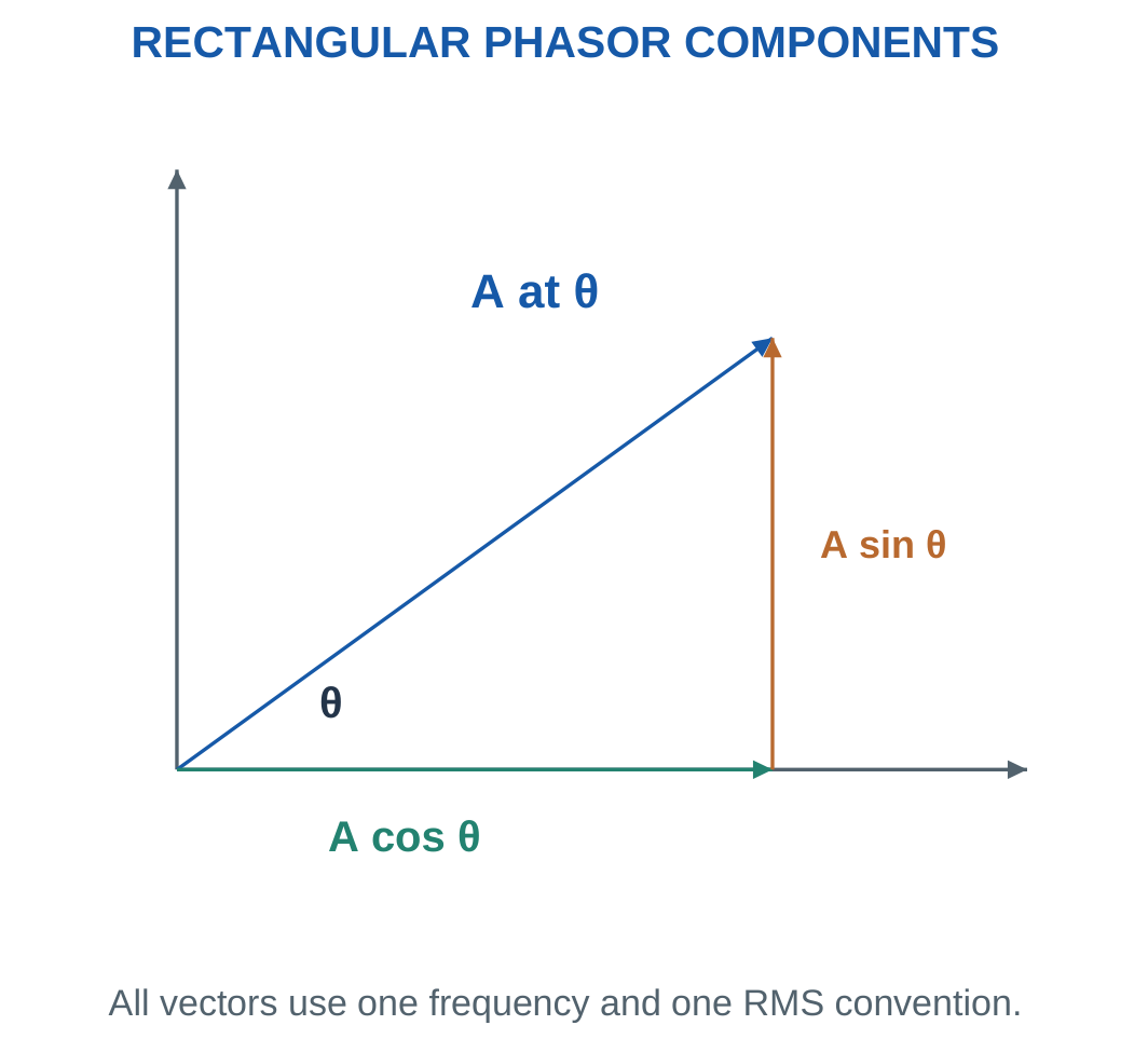
A polar phasor A at angle θ becomes:
A cos θ + jA sin θ
For rectangular form a + jb:
Magnitude = √(a² + b²)
The angle must be selected using both component signs:
θ = atan2(b, a)

Selecting a Convenient Form
Addition and subtraction are easiest in rectangular form. Add real components separately from imaginary components.
Multiplication and division are easiest in polar form. Multiply or divide magnitudes and add or subtract angles.
For AC Ohm’s law:
I = V/Z
Current angle is voltage angle minus impedance angle.
A non-negative magnitude does not identify the quadrant. A phasor with negative real part cannot be assigned a small first-quadrant angle merely because a simple inverse-tangent calculation returns one.
Retain sufficient digits during conversion. Early rounding can create noticeable errors when reconstructing voltage or power.
Worked Problem 2.20: Convert 30 + j40
Magnitude:
√(30² + 40²).
Magnitude = 50 V.
Angle:
atan2(40, 30).
Angle = 53.1301°.
Therefore:
30 + j40 = 50 at 53.1301° V.
Multiplying by j:
j(30 + j40) = −40 + j30.
The magnitude remains 50 V and the angle increases by 90°.
Worked Problem 2.21: Convert 24 − j32
Magnitude:
√(24² + 32²).
Magnitude = 40 V.
Angle:
atan2(−32, 24).
Angle = −53.1301°.
Multiplication by j gives:
j(24 − j32) = 32 + j24.
The resulting phasor remains 40 V in magnitude, with angle +36.8699°.
The operation rotates the vector without changing its RMS length.
Worked Problem 2.22: Convert −60 + j80
Magnitude:
√(60² + 80²).
Magnitude = 100 V.
The signs place the phasor in the second quadrant.
Angle = 126.87°.
Multiplication by j:
j(−60 + j80) = −80 − j60.
Its angle is 216.87°, equivalently −143.13°. Both describe the same direction modulo one complete turn.
Worked Problem 2.23: Convert −12 − j5
Magnitude:
√(12² + 5²).
Magnitude = 13 V.
Using both signs:
Angle = −157.38°.
Multiplication by j gives:
j(−12 − j5) = 5 − j12.
The magnitude remains 13 V. The angle increases by 90°, giving −67.38°.
Quadrant information is essential even when the ratio of components looks numerically simple.
8. Adding AC Voltages Correctly
Kirchhoff’s laws apply instant by instant in AC circuits.
In sinusoidal steady state at one frequency, the same laws can be expressed using phasors. Phasor addition automatically accounts for differences in timing.
Two in-phase voltages add arithmetically. Opposite-phase voltages subtract algebraically.
For two voltages 90° apart:
Vresultant = √(V1² + V2²)
For arbitrary separation δ:
Vresultant = √(V1² + V2² + 2V1V2 cos δ)

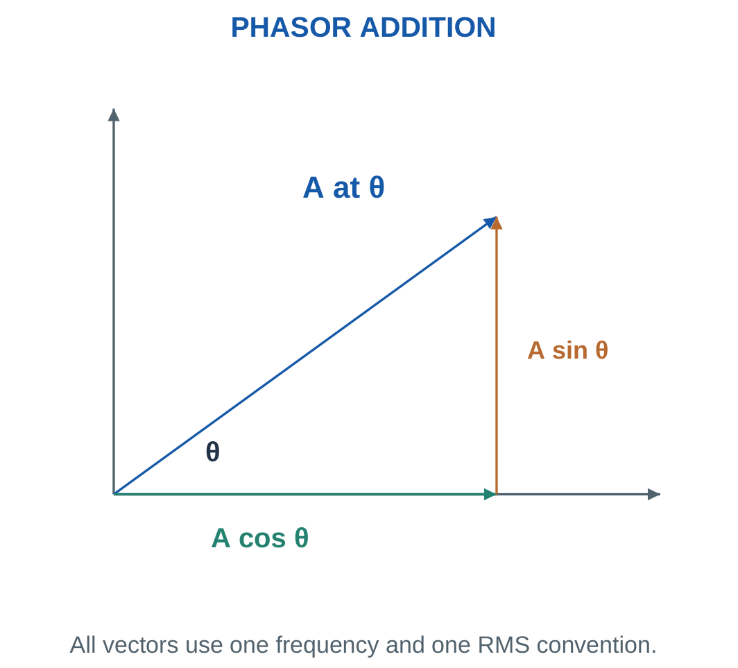
If a resistor drop is 60 V RMS and a series inductor drop is 80 V RMS, the supply magnitude is 100 V RMS.
It is not 140 V because the two component voltages reach their peaks at different times.
Instantaneous signed voltages still satisfy KVL. The phasor calculation is a compact representation of that time-dependent sum.
Reliable Addition Procedure
Choose one common reference. Convert each phasor into rectangular form. Add real parts and imaginary parts separately.
Convert the final result to magnitude and angle only after the rectangular sum is complete.
For subtraction, subtract both components or reverse the subtracted vector. Do not subtract magnitudes unless the vectors lie on the same line.
Worked Problem 2.24: Perpendicular Voltages
Problem: V1 = 60 V at 0° and V2 = 80 V at +90°.
V1 = 60 + j0.
V2 = 0 + j80.
Total:
V = 60 + j80 V.
Magnitude:
100 V.
Angle:
atan2(80, 60).
53.1301°.
The resultant is:
100 V at 53.1301°.
Worked Problem 2.25: Equal Voltages Separated by 60°
Problem: Add 100 V at 0° and 100 V at +60°.
Second phasor:
100 cos 60° + j100 sin 60°.
V2 = 50 + j86.6025 V.
Total:
V = 150 + j86.6025 V.
Magnitude:
173.205 V.
Angle:
30°.
The resultant lies midway between the equal-magnitude phasors, providing a useful symmetry check.
Worked Problem 2.26: A Negative Second Angle
Problem: Add 120 V at 0° and 70 V at −40°.
V2 = 70 cos(−40°) + j70 sin(−40°).
V2 = 53.6231 − j44.9951 V.
Total:
V = 173.623 − j44.9951 V.
Magnitude:
179.359 V.
Phase:
−14.5288°.
The negative imaginary sum places the resultant below the reference axis.
Worked Problem 2.27: Opposite-Phase Voltages
Problem: Add 80 V at 0° and 50 V at 180°.
V1 = 80 + j0.
V2 = −50 + j0.
Total:
V = 30 + j0 V.
Therefore:
Resultant = 30 V at 0°.
This is a case where scalar subtraction is valid because the phasors are collinear and opposite.
Worked Problem 2.28: A 30° Contribution
Problem: Add 90 V at 0° and 40 V at +30°.
V2 = 34.641 + j20 V.
Total:
V = 124.641 + j20 V.
Magnitude:
126.235 V.
Angle:
9.11602°.
The angle is closer to the larger reference phasor, as expected from the relative magnitudes.
9. AC Through a Pure Resistor
An ideal linear resistor obeys:
v = Ri
at every instant.
If:
v = Vm sin ωt
then:
i = (Vm/R) sin ωt
Voltage and current are in phase. Their corresponding zero crossings and peaks occur at the same times.
The RMS relation is:
V = IR


Resistance gives a purely real impedance:
Z = R
Power factor is unity.
Reactive power is zero.
Active power is:
P = VI = I²R = V²/R
Instantaneous power is:
p = VmIm sin² ωt
Since sin² is non-negative, an ideal passive resistor never returns energy to the source.

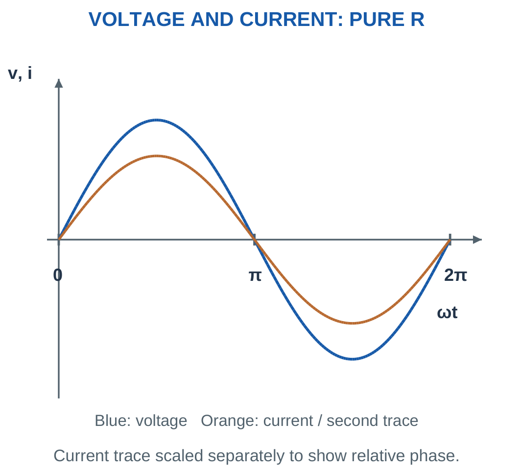
Using the identity sin² α = (1 − cos 2α)/2:
p = VI(1 − cos 2ωt)
Here V and I are RMS values.
The mean power is VI. Maximum instantaneous power is 2VI. At a zero crossing, instantaneous power is zero, but average heating remains positive.
Model Condition
Resistance is treated as independent of frequency and temperature in the ideal calculations.
A real heating element can change resistance as temperature changes. Use the operating resistance supplied in the problem rather than silently introducing an additional temperature model.
Worked Problem 2.29: Resistive Current and Pulsating Power

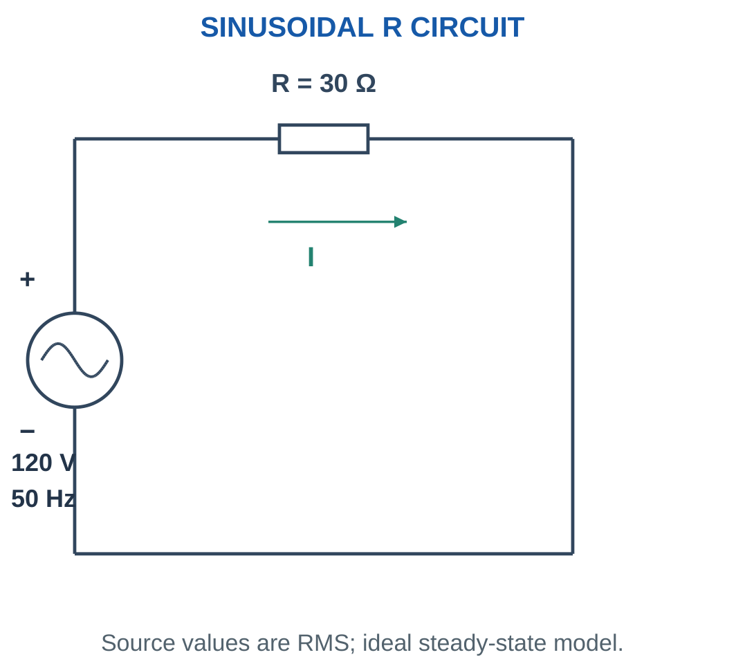
I = V/R = 120/30.
I = 4 A in phase.
Peak current:
Im = √2 × 4.
Im = 5.65685 A.
Mean power:
P = 120 × 4.
P = 480 W.
Maximum instantaneous power:
pmax = 960 W.
Energy in three hours:
W = 480 × 3/1000.
W = 1.44 kWh.
Power varies at 100 Hz, twice the 50 Hz supply frequency.
Worked Problem 2.30: A 230 V Resistive Load


I = 230/46.
I = 5 A.
Peak current:
Im = 7.07107 A.
Average power:
P = 230 × 5.
P = 1150 W.
Maximum instantaneous power:
2300 W.
Energy in three hours:
3.45 kWh.
Voltage and current remain in phase, so the apparent power in VA is numerically equal to active power in watts.
Worked Problem 2.31: A 48 V Resistive Load


I = 48/12.
I = 4 A.
Peak current:
5.65685 A.
Average power:
P = 48 × 4.
P = 192 W.
Maximum instantaneous power:
384 W.
Energy in three hours:
0.576 kWh.
The current matches problem 2.29, but the lower supply voltage and lower resistance produce a smaller power.
10. AC Through a Pure Inductor
An ideal inductor obeys:
v = L di/dt
under the passive sign convention.
Differentiation advances the phase of a sine wave by 90°. Therefore voltage leads current by 90°.
Equivalently:
Inductor current lags voltage by 90°.
Inductive reactance is:
XL = ωL = 2πfL
Its unit is the ohm.
Inductive impedance is:
ZL = jXL

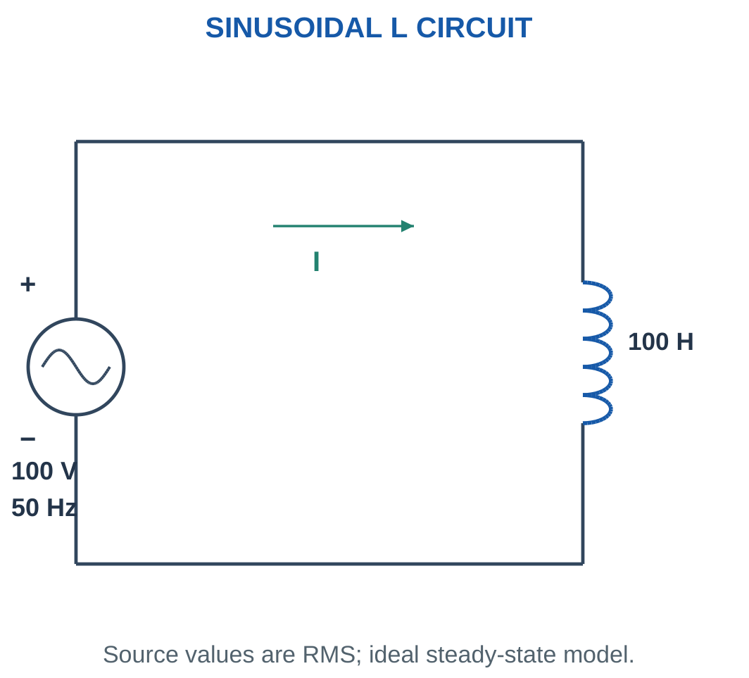
For voltage at zero degrees:
I = V/XL at −90°
Increasing frequency increases reactance for a fixed inductance. At a fixed RMS voltage, this reduces current.
An ideal inductor stores magnetic energy:
w = Li²/2
It absorbs energy as current magnitude increases and returns energy as current magnitude decreases.

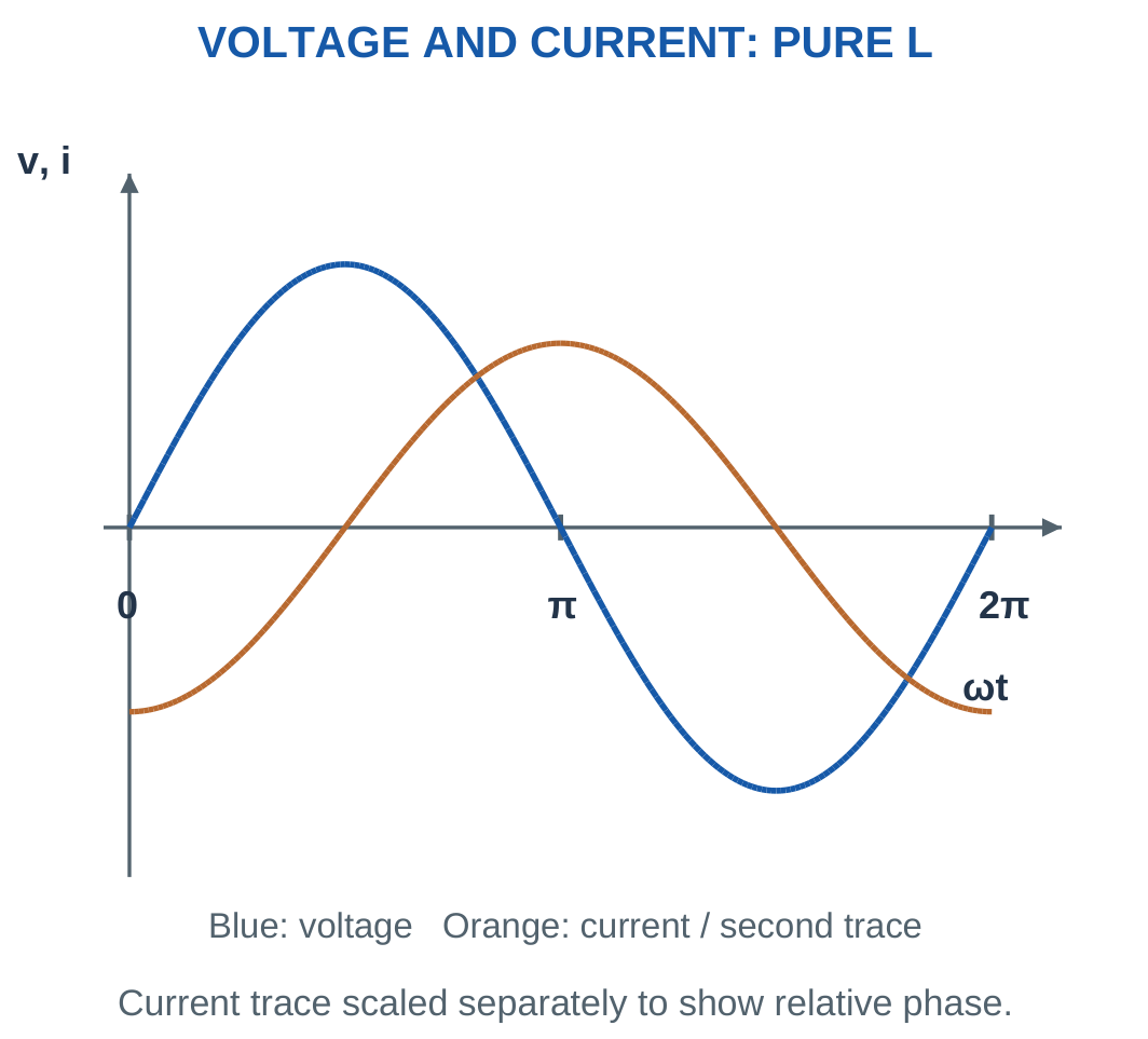
Average active power is zero:
P = VI cos 90° = 0
Reactive power is positive:
Q = VI = I²XL
A real coil has winding resistance and other losses. When resistance is supplied, analyse it as an RL model rather than assigning an exact 90° phase angle.
At a current peak, di/dt is zero, so ideal inductor voltage is zero. At a current zero crossing, the current slope has greatest magnitude and voltage magnitude is maximum.
Worked Problem 2.32: Inductive Current and Magnetic Energy


XL = 2π × 50 × 0.1.
XL = 31.4159 Ω.
Current:
I = 100/31.4159.
I = 3.1831 A at −90°.
Peak current:
Im = 4.50158 A.
Active power:
P = 0 W.
Reactive power:
Q = 100 × 3.1831.
Q = +318.31 var.
Apparent power:
S = 318.31 VA.
Maximum stored energy:
wmax = LIm²/2.
wmax = 1.01321 J.
Energy returns to zero when current crosses zero.
Inductor Winding


An inductive component links current with magnetic energy. Its voltage-current relationship depends on frequency and the selected model.
Winding resistance and core effects can make a real component differ from a pure inductor. The physical presence of a coil is not sufficient justification for ignoring its losses.
Worked Problem 2.33: Inductor at 60 Hz
Problem: An ideal 0.08 H inductor is connected to 48 V RMS at 60 Hz.
XL = 2π × 60 × 0.08.
XL = 30.1593 Ω.
I = 48/30.1593.
I = 1.59155 A lagging by 90°.
Peak current:
Im = 2.25079 A.
Average active power:
0 W.
Reactive power:
Q = +76.3944 var.
Apparent power:
S = 76.3944 VA.
Maximum magnetic energy:
wmax = 0.08 × 2.25079²/2.
wmax = 0.202642 J.
11. AC Through a Pure Capacitor
An ideal capacitor obeys:
i = C dv/dt
Current depends on the rate of change of voltage.
For a sine voltage, differentiation advances current by 90°:
Capacitor current leads voltage by 90°.
The capacitive reactance magnitude is:
XC = 1/(ωC) = 1/(2πfC)
The impedance is:
ZC = −jXC

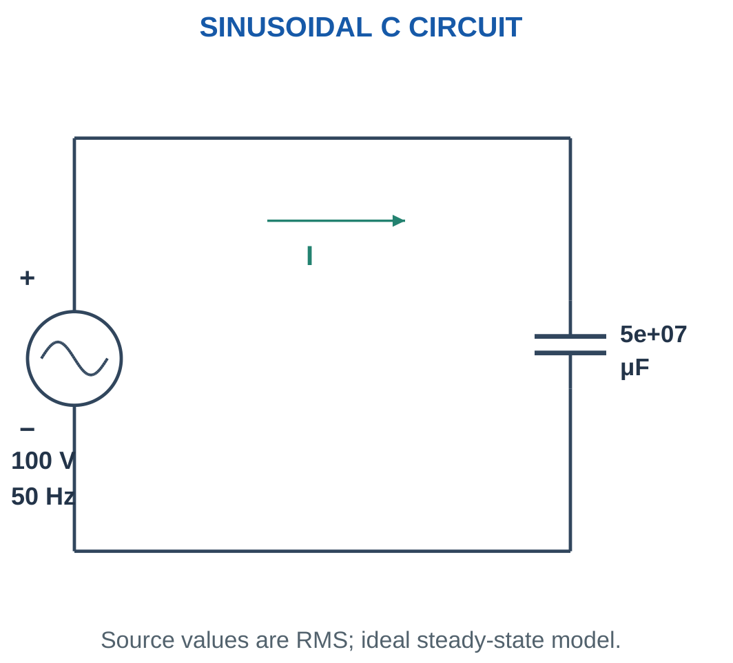
For a voltage phasor at zero degrees:
I = V/XC at +90°
Charge alternately accumulates on and leaves the plates. Conduction through the ideal dielectric is not required for current at the external terminals.
The capacitor stores electric-field energy:
w = Cv²/2
Average active power is zero. Signed reactive power is negative:
Q = −VI = −I²XC


At a voltage peak, dv/dt is zero, so current is zero. At a voltage zero crossing, current magnitude is greatest.
Increasing frequency reduces XC for a fixed capacitance. At fixed RMS voltage, capacitor current increases.
Sign and Unit Discipline
XC is a positive reactance magnitude. Its impedance contribution is −jXC.
Do not insert a negative XC and then apply another negative sign.
Convert microfarads before substitution:
1 μF = 10⁻⁶ F
A missing conversion can create an error of a million in calculated reactance or capacitance.
Worked Problem 2.34: Capacitor Current and Electric Energy


C = 20 × 10⁻⁶ F.
XC = 1/(2π × 50 × 20 × 10⁻⁶).
XC = 159.155 Ω.
I = 100/159.155.
I = 0.628319 A leading by 90°.
Peak current:
Im = 0.888577 A.
Active power:
P = 0 W.
Reactive power:
Q = −62.8319 var.
Apparent power:
S = 62.8319 VA.
Maximum stored energy:
wmax = CVm²/2 = CV².
wmax = 0.2 J.
Worked Problem 2.35: Capacitor at 230 V RMS
Problem: A 10 μF ideal capacitor is connected to 230 V RMS at 50 Hz.
C = 10⁻⁵ F.
XC = 1/(2π × 50 × 10⁻⁵).
XC = 318.31 Ω.
I = 230/318.31.
I = 0.722566 A leading.
Peak current:
Im = 1.02186 A.
Average active power:
0 W.
Reactive power:
Q = −166.19 var.
Apparent power:
S = 166.19 VA.
Maximum electric energy:
wmax = CV².
wmax = 0.529 J.
Film Capacitors for AC Circuits


Capacitance, operating voltage and service rating must be identified from the stated data. Case shape alone does not establish an appropriate AC operating condition.
The analytical model describes ideal energy storage. Practical dielectric loss or leakage is included only when the problem supplies a corresponding model.
12. Comparison of Ideal Resistance, Inductance and Capacitance
The same sinusoidal supply can produce different current phases because each element has a different constitutive relationship.
A resistor relates voltage directly to current. An inductor relates voltage to the rate of current change. A capacitor relates current to the rate of voltage change.
| Property | Pure R | Pure L | Pure C |
|---|---|---|---|
| Impedance | R | jωL | −j/(ωC) |
| Current phase | In phase | Lags 90° | Leads 90° |
| Mean active power | VI | Zero | Zero |
| Reactive power | Zero | +VI | −VI |
| Main action | Dissipation | Magnetic storage | Electric storage |
| Ideal power factor | Unity | Zero lagging | Zero leading |

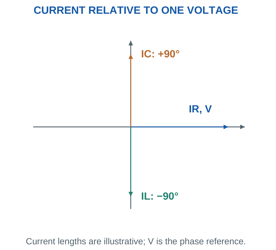
The memory aids ELI and ICE can help recall these relationships.
ELI places voltage E ahead of current I for an inductor L.
ICE places current I ahead of voltage E for a capacitor C.
The differential equations provide the explanation, while the memory aids simply help recall it.
An ideal reactive element can carry nonzero RMS current without absorbing average active power. It stores and returns energy rather than continuously converting it into heat.
Worked Problem 2.36: Recover an Ideal Inductance
Problem: At 50 Hz, an ideal inductor takes 2 A RMS from 100 V RMS.
XL = V/I.
XL = 100/2.
XL = 50 Ω.
L = XL/(2πf).
L = 0.159155 H.
Active power:
P = 0 W.
Apparent power:
S = 200 VA.
Reactive power:
Q = +200 var.
Current lags voltage by 90°.
Worked Problem 2.37: Recover an Ideal Capacitance
Problem: At 50 Hz, a capacitor draws 2 A RMS from 120 V RMS.
XC = 120/2.
XC = 60 Ω.
C = 1/(2π × 50 × 60).
C = 5.30516 × 10⁻⁵ F = 53.0516 μF.
Active power:
P = 0 W.
Apparent power:
S = 240 VA.
Reactive power:
Q = −240 var.
Current leads voltage by 90°.
Worked Problem 2.38: Inductance at 60 Hz
Problem: An ideal inductor takes 2 A from 48 V RMS at 60 Hz.
XL = 48/2.
XL = 24 Ω.
L = 24/(2π × 60).
L = 0.063662 H.
Apparent power:
S = 96 VA.
Reactive power:
Q = +96 var.
Average active power is zero, and current lags the applied voltage by one quarter-cycle.
13. Series RL Circuit: Impedance and Current
A series RL circuit has the same current through resistance and inductance.
Taking current as reference:
VR = IR at 0°
VL = IXL at +90°
The source voltage is their phasor sum.
The impedance is:
Z = R + jXL
Its magnitude is:
|Z| = √(R² + XL²)
Its angle is:
φ = tan⁻¹(XL/R)

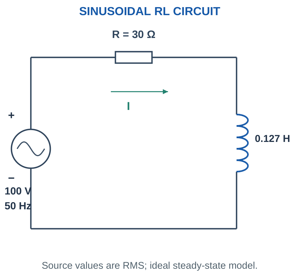


For supply voltage at zero phase:
I = V/|Z| at −φ
Current lags the supply.
Power factor is:
PF = cos φ = R/|Z|
Active power is:
P = I²R
Reactive power is:
Q = I²XL
The inductor changes current magnitude and phase even though its ideal average active power is zero.
Solution Sequence
Convert inductance to henries. Calculate XL at the stated frequency. Form complex impedance and find magnitude and angle.
Calculate current, component voltages and powers. State lagging power factor explicitly.
If only source amplitude changes while R, L and frequency remain fixed, current and component voltages scale proportionally. Impedance and power factor remain unchanged.
Worked Problem 2.39: Complete RL Calculation

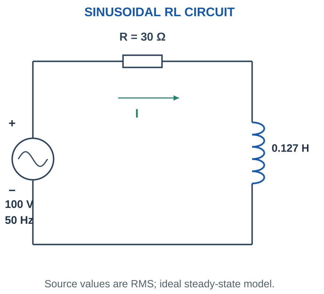
Problem: R = 30 Ω, L = 0.127324 H, V = 100 V RMS and f = 50 Hz.
XL = 2πfL.
XL ≈ 40 Ω.
Z = 30 + j40 Ω.
|Z| = 50 Ω.
φ = tan⁻¹(40/30).
φ = 53.1301°.
Current:
I = 2 A at −53.1301°.
VR = 2 × 30.
VR = 60 V.
VL = 2 × 40.
VL = 80 V.
P = 2² × 30.
P = 120 W.
Q = 2² × 40.
Q = +160 var.
S = 100 × 2.
S = 200 VA.
PF = 0.6 lagging.
Worked Problem 2.40: RL Circuit at 230 V
Problem: R = 46 Ω, L = 0.109817 H, V = 230 V RMS and f = 50 Hz.
XL ≈ 34.5 Ω.
Z = 46 + j34.5 Ω.
|Z| = 57.5 Ω.
φ = 36.8699°.
I = 4 A lagging by 36.8699°.
Component voltages:
VR = 184 V.
VL = 138 V.
Power quantities:
P = 736 W.
Q = +552 var.
S = 920 VA.
PF = 0.8 lagging.
Current peak is 5.65685 A.
For an unshifted supply sine:
i = 5.65685 sin(314.159t − 0.643501) A
The component-voltage magnitudes satisfy 184² + 138² = 230².
Worked Problem 2.41: RL Circuit at 60 Hz
Problem: R = 24 Ω, L = 0.0848826 H, V = 120 V RMS and f = 60 Hz.
XL ≈ 32 Ω.
Z = 24 + j32 Ω.
|Z| = 40 Ω.
Current:
I = 120/40.
I = 3 A at −53.1301°.
Component voltages:
VR = 72 V.
VL = 96 V.
Power quantities:
P = 216 W.
Q = +288 var.
S = 360 VA.
PF = 0.6 lagging.
Resistive and Inductive Load

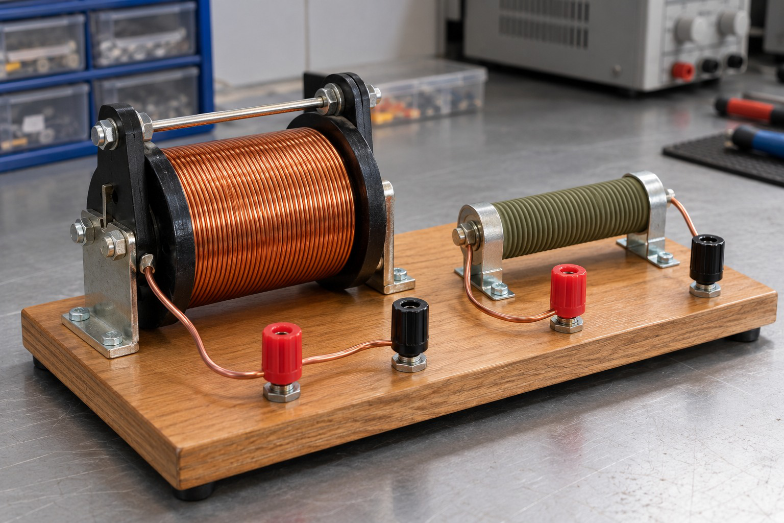
A series RL branch includes both resistance and inductive reactance. The impedance angle determines current lag.
The presence of a coil does not mean its resistance is zero. Use the actual supplied model when deciding whether a branch is pure L or series RL.
14. Series RL Voltage Triangle and Verification
The resistor voltage is in phase with current, while ideal inductor voltage leads that current by 90°.
Therefore:
V² = VR² + VL²
The supply phase relative to current is:
φ = tan⁻¹(VL/VR)

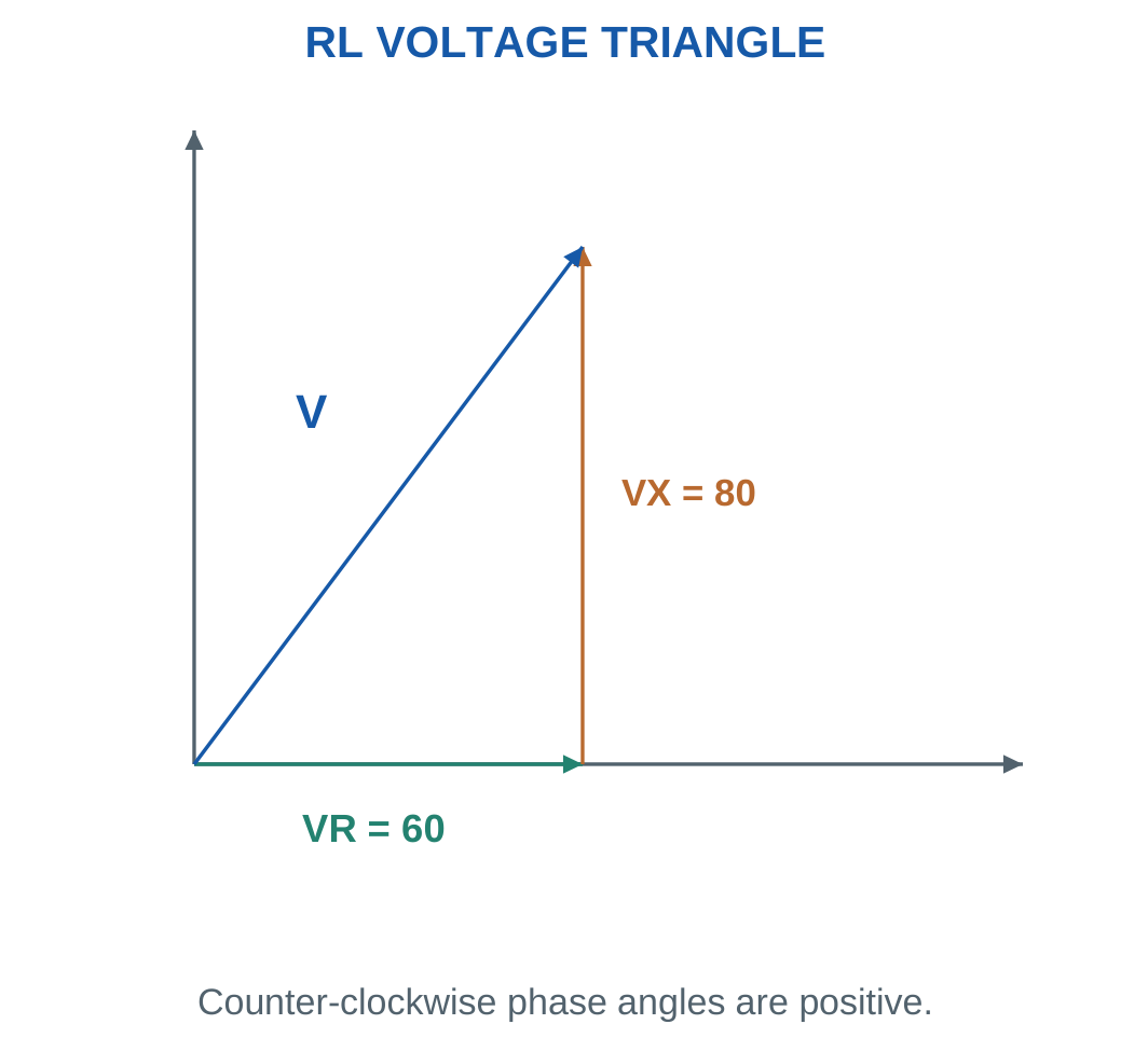
Measured component-voltage magnitudes and known current give:
R = VR/I
XL = VL/I
L = XL/(2πf)
The method assumes the separate resistor and ideal inductive component described in the problem.
A practical coil whose voltage includes both winding resistance and reactance must be treated according to its series equivalent rather than assumed to be an isolated ideal L drop.
Checking a Result
Reconstruct supply magnitude using the voltage triangle.
Independently compare:
P = VI cos φ
with:
P = I²R
Agreement checks magnitude, resistance and RMS convention.
For a positive series RL circuit, current lags by less than 90°, power factor is between zero and one and each component-voltage magnitude is below total supply magnitude.
Worked Problem 2.42: Recover Components from Voltage Drops

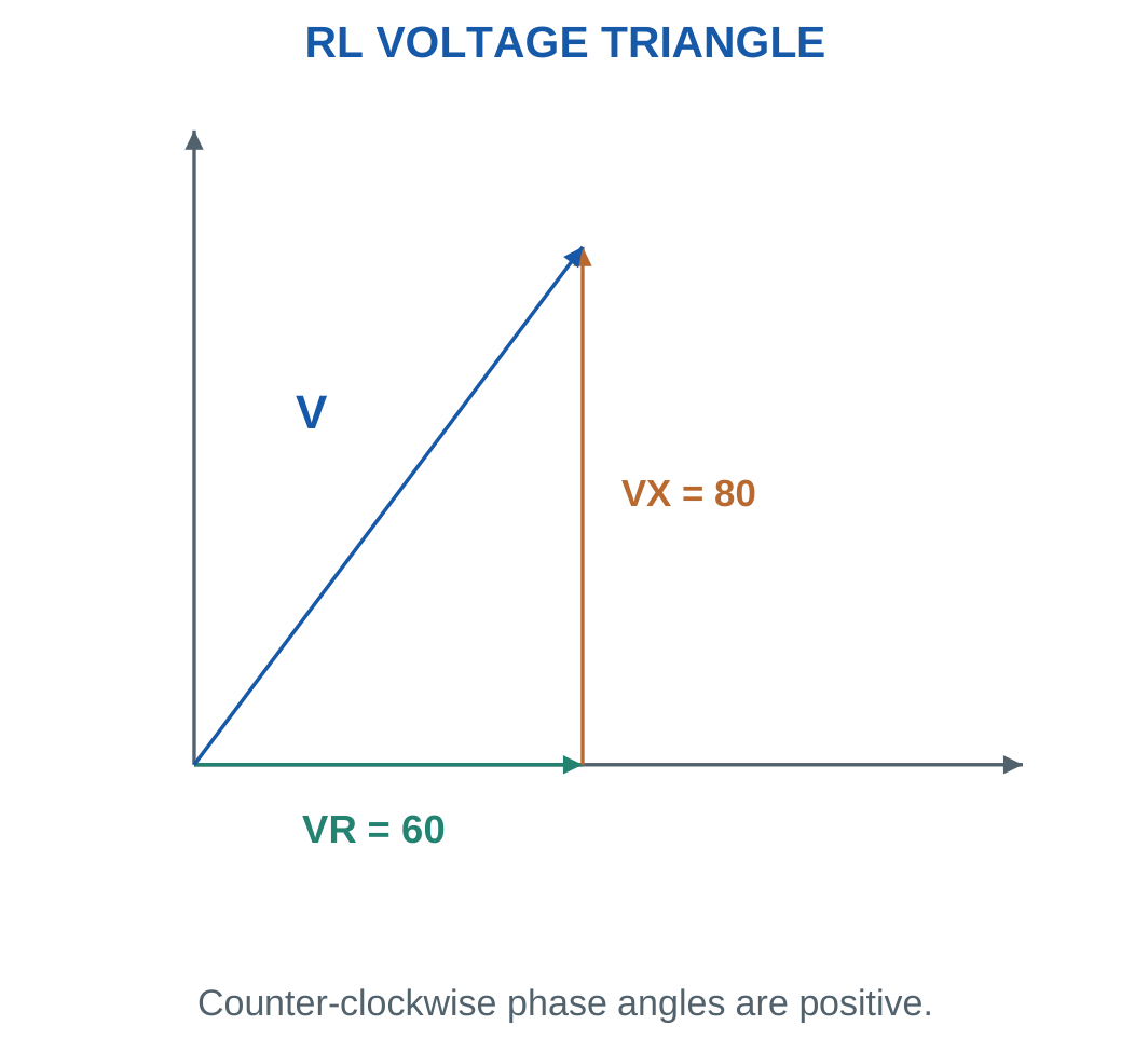
Problem: I = 2 A, f = 50 Hz, VR = 60 V and VL = 80 V.
Supply:
V = √(60² + 80²).
V = 100 V.
Resistance:
R = 60/2.
R = 30 Ω.
Reactance:
XL = 80/2.
XL = 40 Ω.
Inductance:
L = 0.127324 H.
Phase:
53.1301° lagging.
Active power:
P = IVR = 2 × 60.
P = 120 W.
PF = 0.6.
Worked Problem 2.43: Larger Component Drops
Problem: I = 3 A, f = 50 Hz, VR = 90 V and VL = 120 V.
V = √(90² + 120²).
V = 150 V.
R = 90/3.
R = 30 Ω.
XL = 120/3.
XL = 40 Ω.
L = XL/(2πf).
L = 0.127324 H.
Current lags by 53.1301°.
P = 3 × 90.
P = 270 W.
PF = 0.6 lagging.
Worked Problem 2.44: A 60 Hz Voltage Triangle
Problem: I = 1.5 A, f = 60 Hz, VR = 48 V and VL = 36 V.
V = √(48² + 36²).
V = 60 V.
R = 48/1.5.
R = 32 Ω.
XL = 36/1.5.
XL = 24 Ω.
L = 24/(2π × 60).
L = 0.063662 H.
Phase:
36.8699° lagging.
P = 1.5 × 48.
P = 72 W.
PF = 0.8 lagging.
15. Finding an Unknown Coil or Operating Frequency
A practical coil is often represented by series resistance R and ideal inductance L.
If RMS voltage, RMS current and active power are known:
|Z| = V/I
R = P/I²
XL = √(|Z|² − R²)
Then:
L = XL/(2πf)

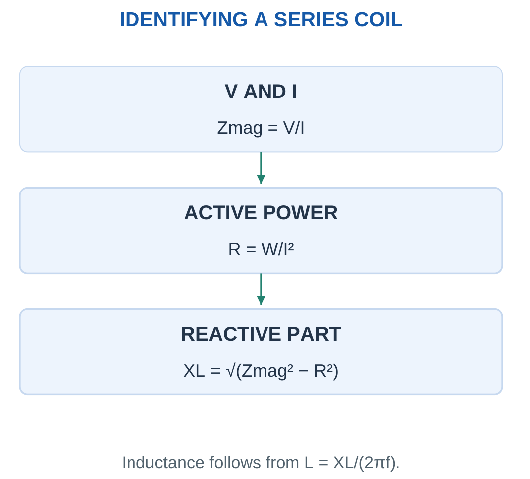
These equations assume a linear series RL model at the stated frequency.
Power factor alone cannot determine both R and L. It provides the ratio R/|Z| and therefore phase information, but another magnitude datum is required.
To determine frequency when V, I, R and L are known, first calculate |Z| = V/I. Recover XL from the impedance triangle and then use:
f = XL/(2πL)
For a specified lag angle:
XL = R tan φ
Therefore:
L = R tan φ/(2πf)
If |Z| is smaller than R, the stated data cannot represent a positive series RL circuit. Check units, RMS conventions and measurement interpretation before proceeding.
Worked Problem 2.45: Identify a Practical Coil
Problem: A coil takes 2 A from 100 V RMS at 50 Hz. Active power is 120 W.
|Z| = 100/2.
|Z| = 50 Ω.
R = 120/2².
R = 30 Ω.
XL = √(50² − 30²).
XL = 40 Ω.
L = 40/(2π × 50).
L = 0.127324 H.
PF = 120/(100 × 2).
PF = 0.6 lagging.
Phase:
53.1301°.
Q = I²XL.
Q = 160 var.
Worked Problem 2.46: Coil at 230 V RMS
Problem: A coil takes 5 A from 230 V RMS at 50 Hz and consumes 920 W.
|Z| = 230/5.
|Z| = 46 Ω.
R = 920/25.
R = 36.8 Ω.
XL = √(46² − 36.8²).
XL = 27.6 Ω.
L = 27.6/(2π × 50).
L = 0.0878535 H.
PF = 0.8 lagging.
φ = 36.8699°.
Q = 25 × 27.6.
Q = 690 var.
Apparent power is 1150 VA.
Worked Problem 2.47: Coil at 60 Hz
Problem: A coil takes 3 A from 120 V RMS at 60 Hz. Active power is 216 W.
|Z| = 120/3.
|Z| = 40 Ω.
R = 216/9.
R = 24 Ω.
XL = √(40² − 24²).
XL = 32 Ω.
L = 32/(2π × 60).
L = 0.0848826 H.
Power factor:
0.6 lagging.
Reactive power:
Q = 288 var.
The physical coil parameters and its operating frequency together determine the observed impedance.
16. Series RC Circuit: Impedance and Current
A series RC circuit has one current through resistance and capacitance.
With current as reference, resistor voltage lies on the positive real axis. Capacitor voltage lags current by 90° and lies on the negative imaginary axis.
Therefore:
Z = R − jXC
Magnitude:
|Z| = √(R² + XC²)
Impedance angle:
θZ = −tan⁻¹(XC/R)


For voltage at zero phase:
θI = −θZ
Therefore current has a positive angle and leads supply voltage.
Power factor is:
PF = R/|Z| leading
Active power:
P = I²R
Reactive power:
Q = −I²XC
Apparent power:
S = VI
Lead and Lag Distinction
Capacitor voltage lags current by 90°. This does not mean series current automatically leads the complete supply voltage by 90°.
The supply is the vector sum of resistor and capacitor voltages. For nonzero resistance, current leads supply by an angle between zero and 90°.
When writing a time equation, use peak current √2I and the positive leading phase relative to the selected supply sine.
Worked Problem 2.48: Complete RC Branch Calculation


Problem: R = 30 Ω, C = 79.5775 μF, V = 100 V RMS and f = 50 Hz.
XC ≈ 40 Ω.
Z = 30 − j40 Ω.
|Z| = 50 Ω.
Impedance angle:
−53.1301°.
Current:
I = 2 A at +53.1301°.
Component voltages:
VR = 60 V.
VC = 80 V.
Power quantities:
P = 120 W.
Q = −160 var.
S = 200 VA.
PF = 0.6 leading.
Worked Problem 2.49: RC Circuit at 230 V
Problem: R = 69 Ω, C = 34.5989 μF, V = 230 V RMS and f = 50 Hz.
XC ≈ 92 Ω.
Z = 69 − j92 Ω.
|Z| = 115 Ω.
Current:
I = 2 A leading by 53.1301°.
Component voltages:
VR = 138 V.
VC = 184 V.
P = 2² × 69.
P = 276 W.
Q = −2² × 92.
Q = −368 var.
S = 230 × 2.
S = 460 VA.
PF = 0.6 leading.
Current waveform:
i = 2.82843 sin(314.159t + 0.927295) A
Worked Problem 2.50: RC Circuit at 60 Hz
Problem: R = 24 Ω, C = 147.366 μF, V = 120 V RMS and f = 60 Hz.
XC ≈ 18 Ω.
Z = 24 − j18 Ω.
|Z| = 30 Ω.
Current magnitude:
I = 120/30.
I = 4 A.
Current leads by:
36.8699°.
Component drops:
VR = 96 V.
VC = 72 V.
Power quantities:
P = 384 W.
Q = −288 var.
S = 480 VA.
PF = 0.8 leading.
Worked Problem 2.51: A 48 V RC Circuit
Problem: R = 9 Ω, C = 265.258 μF, V = 48 V RMS and f = 50 Hz.
XC ≈ 12 Ω.
Z = 9 − j12 Ω.
|Z| = 15 Ω.
I = 48/15.
I = 3.2 A leading by 53.1301°.
VR = 3.2 × 9.
VR = 28.8 V.
VC = 3.2 × 12.
VC = 38.4 V.
P = 92.16 W.
Q = −122.88 var.
S = 153.6 VA.
PF = 0.6 leading.
The current peak is 4.52548 A, so its time equation has that amplitude rather than 3.2 A.
17. Series RC Voltages and Unknown Capacitance
With current as reference:
V = VR − jVC
Therefore:
V² = VR² + VC²
Changing to supply voltage as reference rotates the complete phasor diagram. The physical phase differences remain unchanged.


To recover capacitance from measured capacitor voltage and current:
XC = VC/I
Then:
C = 1/(2πfXC)
If only total V, I and R are supplied:
XC = √[(V/I)² − R²]
Use the positive reactance magnitude in the capacitance equation. The negative sign belongs to the imaginary impedance contribution.
Consistency Checks
For a passive positive-resistance RC circuit, average active power is positive and Q is negative.
A negative impedance angle does not imply negative active power.
At fixed frequency, increasing capacitance reduces reactance. For the same source voltage, current increases and the phase lead decreases.
The capacitor voltage must be recalculated using the new current. It cannot be assumed unchanged simply because the same capacitor position appears in the drawing.
Worked Problem 2.52: Recover RC Components

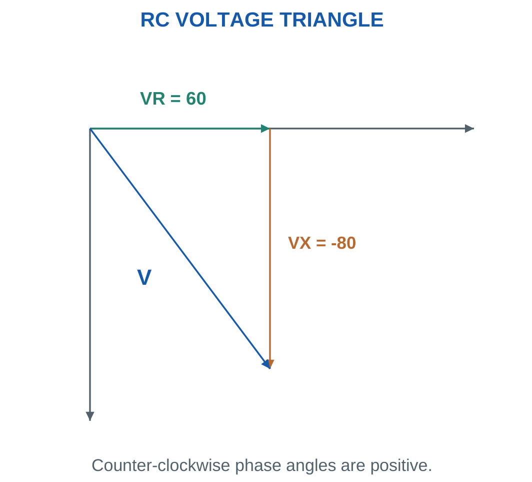
Problem: I = 2 A, f = 50 Hz, VR = 60 V and VC = 80 V.
V = √(60² + 80²).
V = 100 V.
R = 60/2.
R = 30 Ω.
XC = 80/2.
XC = 40 Ω.
C = 1/(2π × 50 × 40).
C = 79.5775 μF.
Current leads supply by 53.1301°.
P = IVR.
P = 120 W.
PF = 0.6 leading.
Worked Problem 2.53: Larger RC Voltage Drops
Problem: I = 3 A, f = 50 Hz, VR = 90 V and VC = 120 V.
V = √(90² + 120²).
V = 150 V.
R = 90/3.
R = 30 Ω.
XC = 120/3.
XC = 40 Ω.
Capacitance:
C = 79.5775 μF.
Phase:
53.1301° leading.
Active power:
P = 3 × 90.
P = 270 W.
PF = 0.6 leading.
Worked Problem 2.54: RC Components at 60 Hz
Problem: I = 1.5 A, f = 60 Hz, VR = 48 V and VC = 36 V.
V = √(48² + 36²).
V = 60 V.
R = 48/1.5.
R = 32 Ω.
XC = 36/1.5.
XC = 24 Ω.
C = 1/(2π × 60 × 24).
C = 110.524 μF.
Current leads by 36.8699°.
P = 1.5 × 48.
P = 72 W.
PF = 0.8 leading.
18. Frequency Dependence of RL and RC Circuits
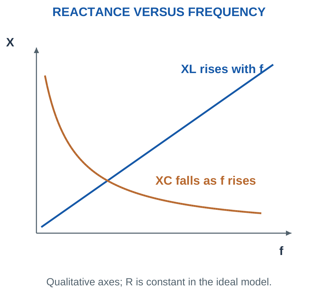
Frequency changes the opposition of reactive components.
For fixed inductance:
XL ∝ f
For fixed capacitance:
XC ∝ 1/f
Resistance remains constant in the ideal model.
Therefore a change in frequency changes impedance magnitude, current magnitude, phase and active power.

For series RL at fixed RMS voltage:
- Increasing frequency increases XL.
- Impedance magnitude increases.
- Current decreases.
- Phase lag increases.
- Power factor decreases.
- Resistor active power decreases.
For series RC at fixed RMS voltage:
- Increasing frequency decreases XC.
- Impedance magnitude decreases.
- Current increases.
- Phase lead decreases.
- Power factor increases.
- Resistor active power increases.
Limiting Behaviour
At very low frequency, a series RL circuit approaches resistive behaviour in the steady sinusoidal model.
At very low frequency, a series RC circuit carries very little sinusoidal current.
At very high frequency, finite-resistance series RC current approaches V/R.
These are steady-state limits. They are not switching-transient equations.
When frequency changes, recalculate reactance, impedance and current before calculating new drops or powers. Physical L and C remain unchanged, but their reactances do not.
Worked Problem 2.55: Lower Frequency in an RL Branch
Problem: R = 30 Ω and XL = 40 Ω at 50 Hz. V = 100 V RMS. Find the response at 25 Hz.
Inductive reactance scales directly with frequency:
XL,new = 40 × 25/50.
XL,new = 20 Ω.
|Z| = √(30² + 20²).
|Z| = 36.0555 Ω.
I = 100/36.0555.
I = 2.7735 A.
PF = 30/36.0555.
PF = 0.83205 lagging.
P = I²R.
P = 230.769 W.
Current increases from its original 2 A because inductive opposition falls.
Worked Problem 2.56: Higher Frequency in an RL Branch
At 100 Hz:
XL,new = 40 × 100/50.
XL,new = 80 Ω.
|Z| = √(30² + 80²).
|Z| = 85.44 Ω.
I = 100/85.44.
I = 1.17041 A.
PF = 30/85.44.
PF = 0.351123 lagging.
P = I² × 30.
P = 41.0959 W.
Doubling frequency does not simply halve current because resistance remains part of impedance.
Worked Problem 2.57: Lower Frequency in an RC Branch
Problem: R = 30 Ω and XC = 40 Ω at 50 Hz. V = 100 V RMS. Find the response at 25 Hz.
Capacitive reactance varies inversely with frequency:
XC,new = 40 × 50/25.
XC,new = 80 Ω.
|Z| = √(30² + 80²).
|Z| = 85.44 Ω.
I = 1.17041 A.
PF = 0.351123 leading.
P = 41.0959 W.
Reducing frequency increases capacitive opposition, so current decreases.
Worked Problem 2.58: Higher Frequency in an RC Branch
At 100 Hz:
XC,new = 40 × 50/100.
XC,new = 20 Ω.
|Z| = √(30² + 20²).
|Z| = 36.0555 Ω.
I = 100/36.0555.
I = 2.7735 A.
PF = 30/36.0555.
PF = 0.83205 leading.
P = I² × 30.
P = 230.769 W.
The current grows toward the limiting value V/R as capacitive reactance becomes smaller.
19. Active Power and Instantaneous Power
Active power is the average rate of energy transfer that is not returned by the ideal reactive exchange.
For sinusoidal RMS voltage and current:
P = VI cos φ
Its unit is the watt.
For the series RL and RC models:
P = I²R
because the ideal reactive element has zero average active power.
Take:
v = √2V sin ωt
and:
i = √2I sin(ωt − φ)
Multiplying and applying the product identity gives:
p = VI[cos φ − cos(2ωt − φ)]

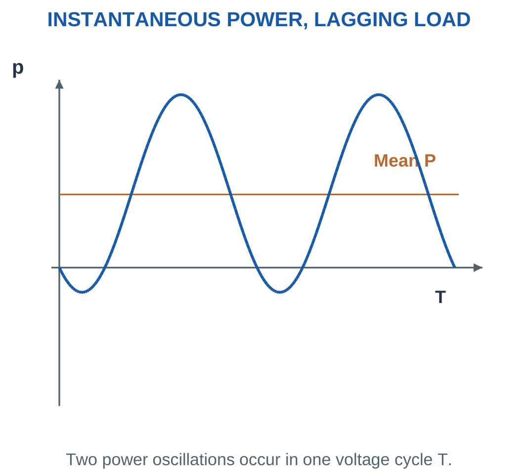
The cosine term has zero average over a complete cycle. Therefore:
Paverage = VI cos φ
Negative instantaneous power represents energy returning toward the source under the passive load reference.
It does not imply negative average power for a passive resistor combined with an ideal inductor or capacitor.
RMS and Peak Conventions
If peak values are used:
P = (VmIm/2) cos φ
If RMS values are used:
P = VI cos φ
Do not add another factor of one half when the values are already RMS.
For a pure resistor, instantaneous power never becomes negative. For a pure reactive element, positive and negative energy-transfer areas cancel over a cycle.
Worked Problem 2.59: Power at 0.8 Lagging PF
Problem: V = 230 V RMS, I = 5 A RMS and PF = 0.8 lagging.
S = VI.
S = 1150 VA.
φ = cos⁻¹0.8.
φ = 36.8699°.
P = 230 × 5 × 0.8.
P = 920 W.
Q = VI sin φ.
Q = +690 var.
Peak values are 325.269 V and 7.07107 A. Substituting them into VmIm cos φ/2 gives the same 920 W.
Worked Problem 2.60: Power at 0.6 Lagging PF
Problem: V = 120 V RMS, I = 10 A RMS and PF = 0.6 lagging.
S = 120 × 10.
S = 1200 VA.
Phase:
53.1301°.
Active power:
P = 720 W.
Reactive power:
Q = +960 var.
Peak voltage is 169.706 V and peak current is 14.1421 A.
The peak-value expression again gives 720 W when exactly one factor of one half is included.
Worked Problem 2.61: A Leading Load
Problem: V = 100 V RMS, I = 8 A RMS and PF = 0.75 leading.
S = 800 VA.
The signed phase is:
φ = −41.4096°.
P = 100 × 8 × 0.75.
P = 600 W.
Q = 800 sin(−41.4096°).
Q = −529.15 var.
Peak values are 141.421 V and 11.3137 A.
The negative reactive power describes capacitive behaviour while active power remains positive.
Worked Problem 2.62: A 0.9 Leading Load
Problem: V = 200 V RMS, I = 4 A RMS and PF = 0.9 leading.
S = 800 VA.
φ = −25.8419°.
P = 200 × 4 × 0.9.
P = 720 W.
Q = 800 sin(−25.8419°).
Q = −348.712 var.
Peak voltage is 282.843 V and peak current is 5.65685 A.
Using peak values with the factor one half reproduces the RMS-based active-power result.
20. Reactive Power, Apparent Power and Complex Power
Apparent power is the product of RMS terminal voltage and current:
S = VI
Its unit is the volt-ampere, VA.
Reactive power for sinusoidal steady state is:
Q = VI sin φ
Its unit is var.
Inductive loads have positive φ and positive Q. Capacitive loads have negative φ and negative Q.
A negative Q does not mean negative active power. It identifies the direction of reactive behaviour under the selected convention.

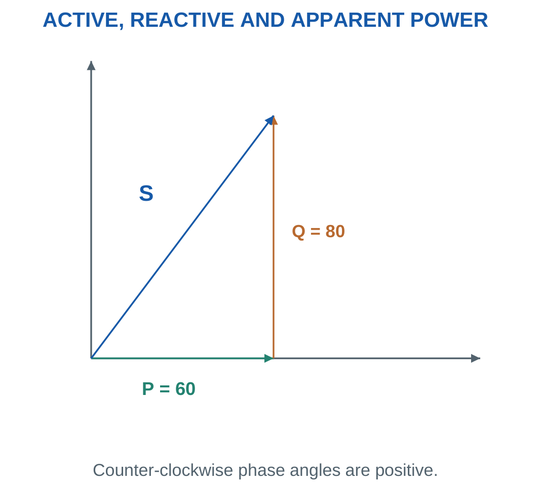
Complex power is:
Scomplex = VI = P + jQ*
The asterisk denotes current conjugation.
The magnitude of complex power is apparent power:
|Scomplex| = S = √(P² + Q²)
Power factor is:
PF = P/S
For positive active power:
tan φ = Q/P
Current conjugation is essential. If voltage is chosen real and current lags, current has a negative imaginary component. Its conjugate makes inductive load Q positive.
Unit Distinctions
Use watts for P, var for Q and VA for S.
Convert kW, kvar and kVA consistently before combining values.
An ideal reactive element can have nonzero S while P is zero. Therefore VI is not generally the active power in watts.
Worked Problem 2.63: Power Triangle from P and Q


Problem: P = 600 W, Q = +800 var and V = 100 V RMS.
S = √(600² + 800²).
S = 1000 VA.
I = S/V.
I = 10 A.
Active current component:
P/V = 6 A.
Reactive current component in complex current:
−jQ/V = −j8 A.
Icomplex = 6 − j8 A.
PF = 0.6 lagging.
φ = 53.1301°.
Worked Problem 2.64: Negative Reactive Power


Problem: P = 1200 W, Q = −900 var and V = 150 V RMS.
S = √(1200² + 900²).
S = 1500 VA.
I = 1500/150.
I = 10 A.
Complex current:
I = P/V − jQ/V.
I = 8 + j6 A.
PF = 0.8 leading.
The signed voltage-minus-current phase is −36.8699°.
Worked Problem 2.65: A 3 kVA Lagging Load

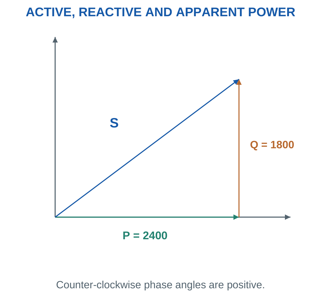
Problem: P = 2400 W, Q = +1800 var and V = 230 V RMS.
S = √(2400² + 1800²).
S = 3000 VA.
I = 3000/230.
I = 13.0435 A.
Active component:
10.4348 A.
Lagging reactive component magnitude:
7.82609 A.
PF = 0.8 lagging.
φ = 36.8699°.
Worked Problem 2.66: A 1 kVA Leading Load
Problem: P = 800 W, Q = −600 var and V = 200 V RMS.
S = √(800² + 600²).
S = 1000 VA.
I = 1000/200.
I = 5 A.
Complex current:
I = 4 + j3 A.
Power factor:
0.8 leading.
The apparent-power magnitude is positive even though reactive power is negative.
21. Power Factor and Current Components
Power factor is:
PF = P/S
For the sinusoidal linear circuits considered here:
PF = cos φ
The numerical magnitude alone does not distinguish leading from lagging.
A load with PF 0.8 may be inductive or capacitive. Additional phase information or a stated circuit model is required.

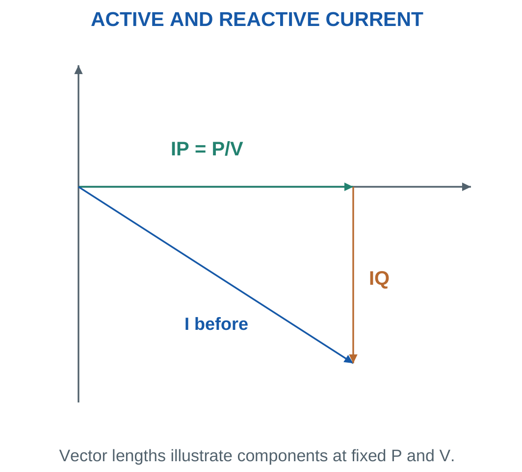
With voltage V at zero phase:
IP = P/V = I cos φ
The complex current is:
Icomplex = P/V − jQ/V
Magnitude is:
I = √[(P/V)² + (Q/V)²]
For fixed active power and voltage:
I = P/(V PF)
Lower power factor requires more RMS source current.
This increases conductor and supply-equipment current requirements. A specified line resistance has loss I²Rline.
Scope of the Cosine Relationship
For distorted nonsinusoidal waveforms, true power factor need not equal only the cosine of a displacement angle.
The present problems assume sinusoidal steady state, so PF = cos φ is appropriate.
Power-factor improvement does not automatically reduce the useful load’s active power. State the quantities held fixed, normally load active power and load-terminal RMS voltage.
Worked Problem 2.67: Separate Current Components
Problem: A 2000 W load operates at 230 V and 0.8 lagging PF.
Total current:
I = 2000/(230 × 0.8).
I = 10.8696 A.
Active component:
IP = P/V.
IP = 8.69565 A.
Lagging component magnitude:
IQ = I√(1 − PF²).
IQ = 6.52174 A.
Complex current:
I = 8.69565 − j6.52174 A.
At unity source PF for the same P and V:
Isource = 8.69565 A.
Useful active load power remains 2000 W.
Worked Problem 2.68: A Lower Initial Power Factor
Problem: A 1200 W load operates at 120 V and 0.6 lagging PF.
I = 1200/(120 × 0.6).
I = 16.6667 A.
Active component:
IP = 1200/120.
IP = 10 A.
Reactive component:
IQ = 13.3333 A lagging.
At unity source power factor:
Isource = 10 A.
The capacitor required to achieve this condition would offset reactive source current. It would not eliminate current in the original inductive branch.
22. Combining Loads Through Active and Reactive Power
For several loads connected to the same single-phase supply, add active powers and signed reactive powers separately.
Ptotal = P1 + P2 + …
Qtotal = Q1 + Q2 + …
Then:
Stotal = √(Ptotal² + Qtotal²)
Isource = Stotal/V

Do not add apparent-power magnitudes indiscriminately.
A 600 W resistor and an ideal 800 var inductor together have apparent power 1000 VA, not 1400 VA. Their current components are perpendicular.
Opposing reactive powers can cancel partly or completely at the source while each branch continues to carry its own current.
This method is particularly convenient when loads are specified by active power and power factor rather than component values.
All combined loads must share the stated frequency and sinusoidal steady-state assumptions.
Worked Problem 2.69: Two Lagging or Unity Loads
Problem: Two loads share 230 V RMS. Load 1 is 1000 W at 0.8 lagging PF. Load 2 is a 600 W unity-PF load.
Q1 = P1 tan(cos⁻¹0.8).
Q1 = 750 var.
Q2 = 0.
Total powers:
Ptotal = 1600 W.
Qtotal = 750 var.
S = √(1600² + 750²).
S = 1767.06 VA.
I = 1767.06/230.
I = 7.68287 A.
PF = 1600/1767.06.
PF = 0.905459 lagging.
Power and Apparent-Power Measurement

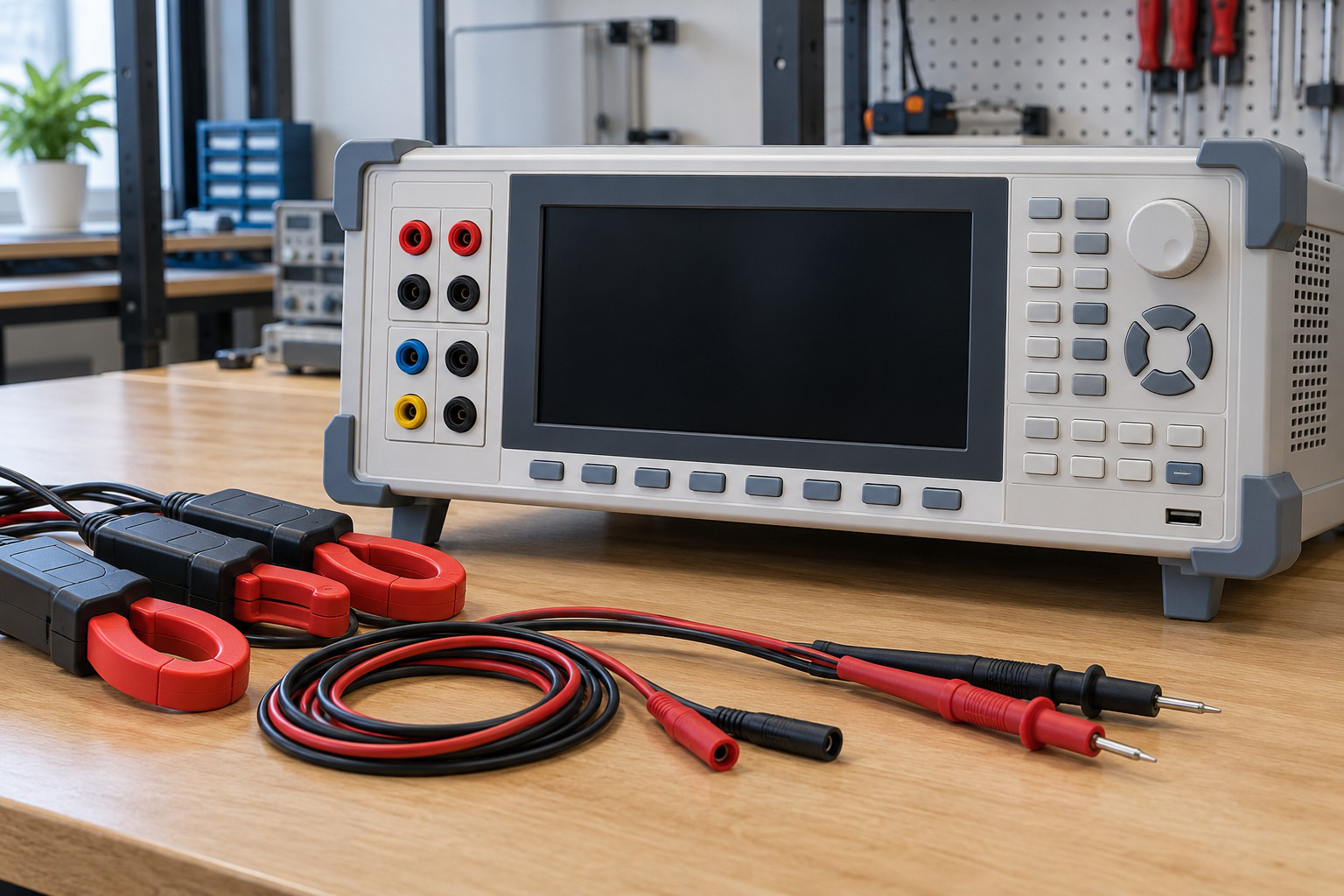
Active, reactive and apparent power are different quantities. A measurement should identify voltage and current conventions, circuit connections and instrument range.
The interpretation of a displayed value depends on the measurement mode and supported waveform conditions.
Worked Problem 2.70: Opposing Reactive Powers
Problem: At 230 V, load 1 is 2000 W at 0.8 lagging PF. Load 2 is 800 W at 0.6 leading PF.
First-load reactive power:
Q1 = +1500 var.
Second-load reactive power:
Q2 = −800 tan(cos⁻¹0.6).
Q2 = −1066.67 var.
Total:
P = 2800 W.
Q = 433.333 var.
S = √(2800² + 433.333²).
S = 2833.33 VA.
I = S/230.
I = 12.3188 A.
PF = 0.988235 lagging.
The leading load offsets most, but not all, of the lagging reactive power.
Worked Problem 2.71: Resistor and Ideal Capacitor
Problem: A 600 W unity-PF load and a capacitor supplying 800 var share 100 V RMS.
Total active power:
P = 600 W.
Signed reactive power:
Q = −800 var.
S = √(600² + 800²).
S = 1000 VA.
I = 1000/100.
I = 10 A.
PF = 600/1000.
PF = 0.6 leading.
The capacitor has no ideal average active power, but it increases source-current magnitude relative to the 6 A resistive current alone.
23. Why a Shunt Capacitor Improves Lagging Power Factor
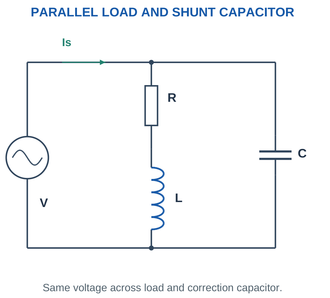
An inductive load draws both an in-phase current component and a lagging reactive component.
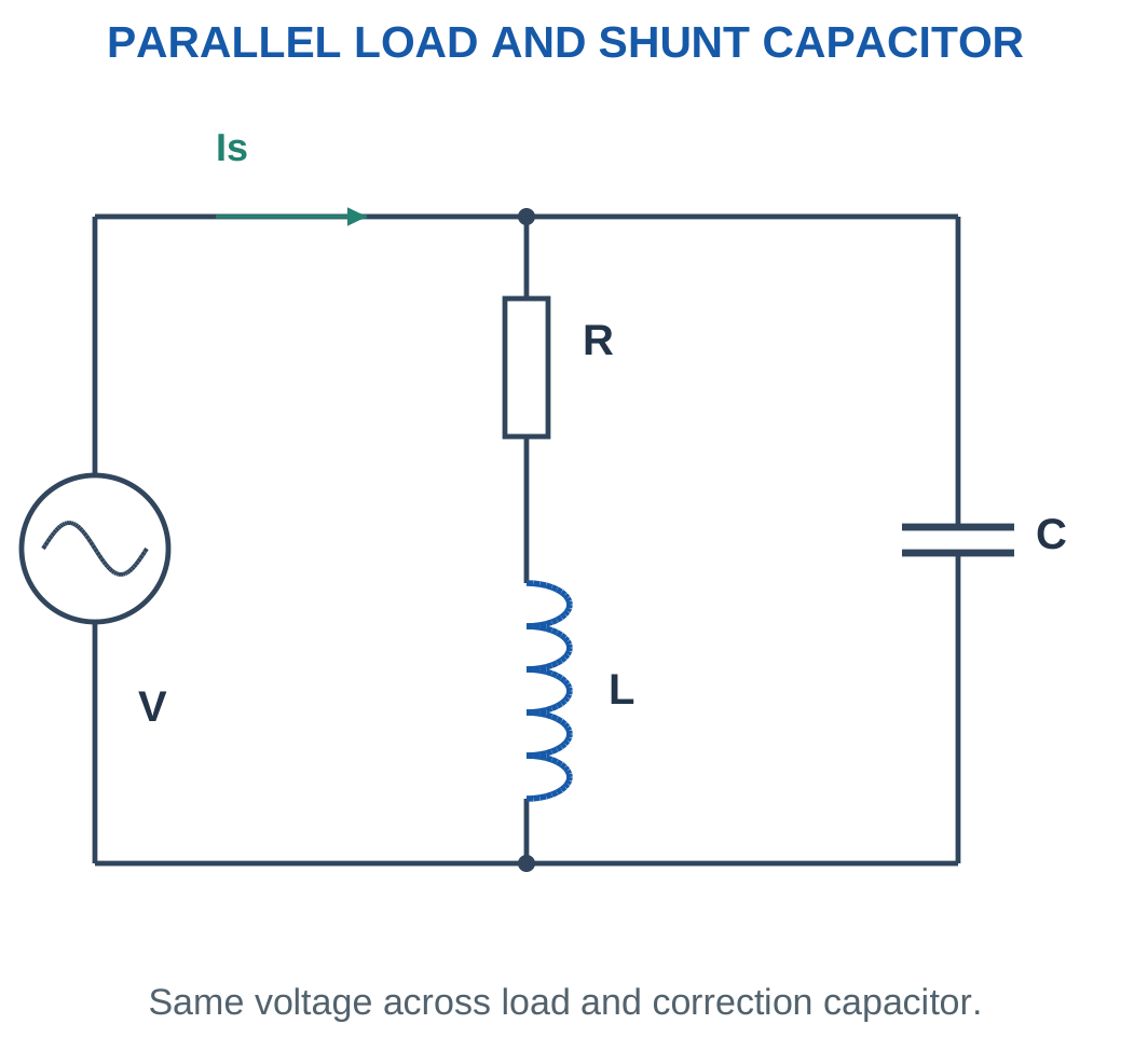
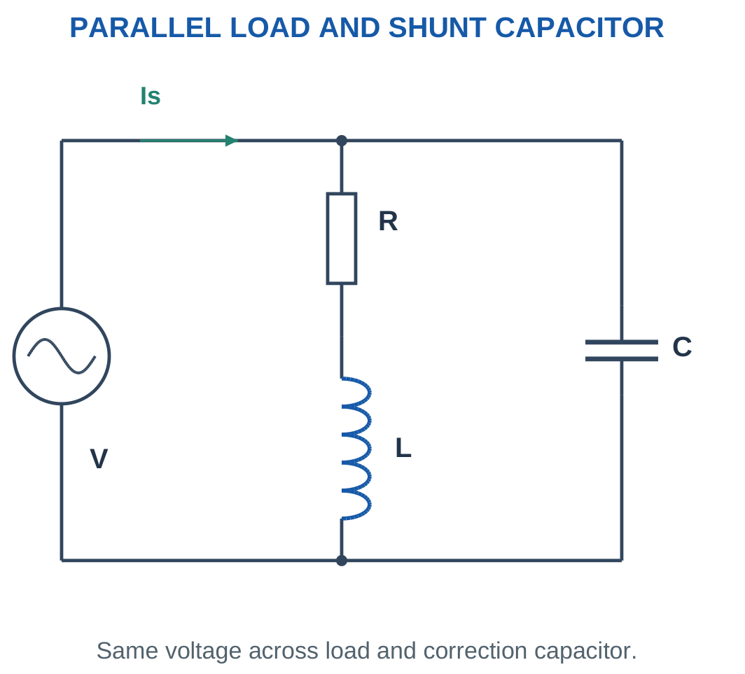
A capacitor connected in parallel across the same supply draws leading reactive current.
The leading and lagging components oppose at the supply terminals.


With an ideal capacitor and unchanged terminal voltage, the original load retains its own active and reactive powers.
The capacitor contributes zero mean active power and negative reactive power.
If Qc is the positive compensation size:
Qsource = Qload − Qc
Source active power remains P in the ideal model.


The source current falls because the magnitude of the vector sum falls.
The capacitor does not remove resistance from the original load. It changes the combined load-plus-capacitor power factor seen by the source.
A series capacitor is a different arrangement because it changes the load branch itself. The correction formulas here apply to a shunt connection.
Power-Factor Capacitor Hardware

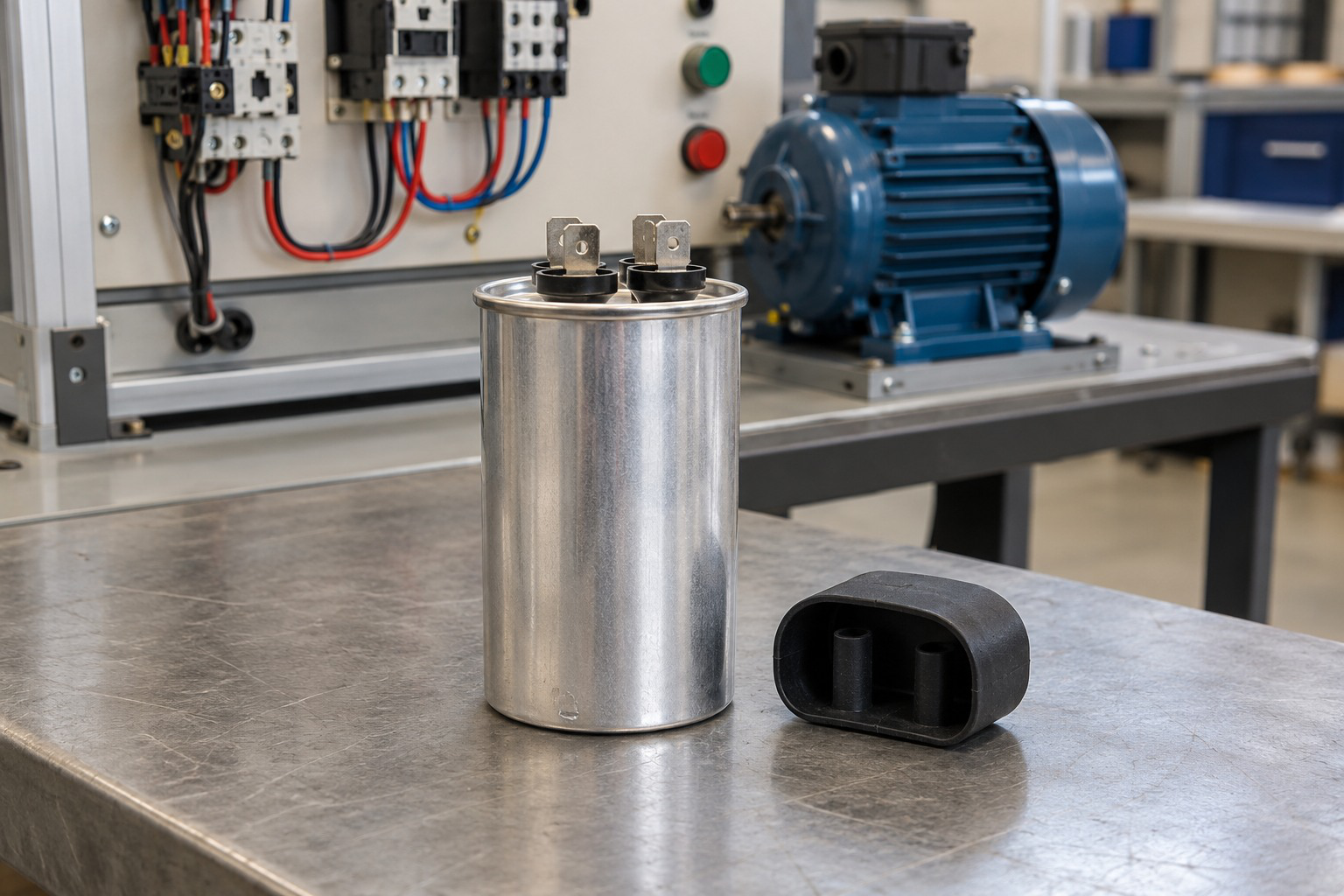
The numerical calculation determines required reactive compensation under the specified voltage and frequency.
Actual component selection also depends on appropriate voltage and service ratings. The ideal calculation is a circuit model rather than a complete equipment design.
Worked Problem 2.72: Improve 0.6 to 0.9 Lagging
Problem: A 1200 W load operates at 120 V RMS, 60 Hz and 0.6 lagging PF. Improve source PF to 0.9 lagging.
Original angle:
φ1 = 53.1301°.
Original reactive power:
Q1 = 1200 tan φ1.
Q1 = 1600 var.
Target angle:
φ2 = 25.8419°.
Target reactive power:
Q2 = 581.187 var.
Compensation:
Qc = Q1 − Q2.
Qc = 1018.81 var.
Capacitance:
C = Qc/(2πfV²).
C = 187.673 μF.
Initial current:
I1 = 16.6667 A.
Corrected current:
I2 = 11.1111 A.
Capacitor current:
Ic = Qc/V.
Ic = 8.49011 A leading.
The corrected current is not I1 minus Ic arithmetically because those current phasors have different directions.
Worked Problem 2.73: Improve 0.75 to 0.95 Lagging
Problem: P = 3000 W, V = 250 V, f = 50 Hz, PF1 = 0.75 lagging and PF2 = 0.95 lagging.
Original angle:
41.4096°.
Original reactive power:
Q1 = 2645.75 var.
Target angle:
18.1949°.
Target reactive power:
Q2 = 986.052 var.
Compensation:
Qc = 1659.7 var.
Capacitance:
C = 84.5278 μF.
Initial current:
I1 = 16 A.
Corrected current:
I2 = 12.6316 A.
Capacitor current:
Ic = 6.6388 A leading.
The active current component remains P/V = 12 A before and after ideal correction.
24. Sizing the Correction Capacitor
For a lagging load with active power P:
Q1 = P tan φ1
For a less-lagging target:
Q2 = P tan φ2
The positive compensation size is:
Qc = P(tan φ1 − tan φ2)
For a single-phase shunt capacitor:
Ic = ωCV.
Therefore:
Qc = VIc = ωCV².
Hence:
C = Qc/(2πfV²)

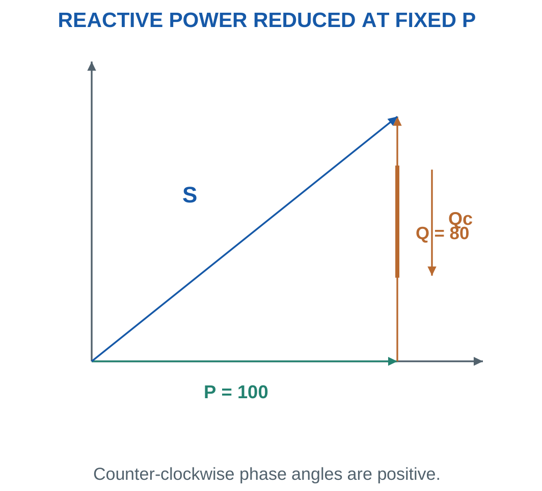
Use P in watts, Qc in var, frequency in hertz and voltage in RMS volts to obtain capacitance in farads.
No additional factor of three belongs in this single-phase formula.
If inverse angles are avoided:
tan φ = √(1 − PF²)/PF
for a positive lagging power factor.
At unity target PF:
φ2 = 0
Q2 = 0
Qc = Q1
After finding capacitance, verify corrected source current using P/(VPF2) and independently using active and residual reactive current components.
Worked Problem 2.74: A 5 kW Load

Problem: P = 5000 W, V = 230 V, f = 50 Hz, PF1 = 0.7 and PF2 = 0.95, both lagging.
φ1 = cos⁻¹0.7.
φ1 = 45.573°.
Q1 = 5101.02 var.
φ2 = cos⁻¹0.95.
φ2 = 18.1949°.
Q2 = 1643.42 var.
Qc = Q1 − Q2.
Qc = 3457.6 var.
C = 3457.6/(2π × 50 × 230²).
C = 208.051 μF.
Currents:
I1 = 31.0559 A.
I2 = 22.8833 A.
Ic = 15.033 A leading.
Worked Problem 2.75: Improve 0.6 to 0.8 Lagging

Problem: P = 1000 W, V = 100 V, f = 50 Hz, PF1 = 0.6 and PF2 = 0.8 lagging.
Q1 = 1333.33 var.
Q2 = 750 var.
Qc = 1333.33 − 750.
Qc = 583.333 var.
Capacitance:
C = 185.681 μF.
Initial source current:
I1 = 16.6667 A.
Corrected source current:
I2 = 12.5 A.
Capacitor current:
Ic = 5.83333 A leading.
The residual source reactive current is Q2/V = 7.5 A lagging.
Worked Problem 2.76: Correction to Unity
Problem: P = 2400 W, V = 240 V, f = 60 Hz and PF1 = 0.8 lagging. Correct to unity.
Original reactive power:
Q1 = 2400 tan(cos⁻¹0.8).
Q1 = 1800 var.
At unity:
Q2 = 0.
Therefore:
Qc = 1800 var.
C = 1800/(2π × 60 × 240²).
C = 82.8932 μF.
Initial current:
I1 = 12.5 A.
Final source current:
I2 = 10 A.
Capacitor current:
Ic = 7.5 A leading.
The original lagging reactive component is cancelled at the source, while reactive currents continue in the individual branches.
Worked Problem 2.77: Improve 0.65 to 0.9 Lagging
Problem: P = 1500 W, V = 200 V and f = 50 Hz.
Original PF is 0.65 lagging, giving:
φ1 = 49.4584°.
Q1 = 1753.69 var.
Target PF is 0.9 lagging, giving:
φ2 = 25.8419°.
Q2 = 726.483 var.
Compensation:
Qc = 1027.21 var.
Capacitance:
C = 81.7429 μF.
Initial current:
I1 = 11.5385 A.
Corrected current:
I2 = 8.33333 A.
Capacitor current:
Ic = 5.13606 A leading.
The unchanged active component is P/V = 7.5 A.
25. Overcorrection and Changing Conditions
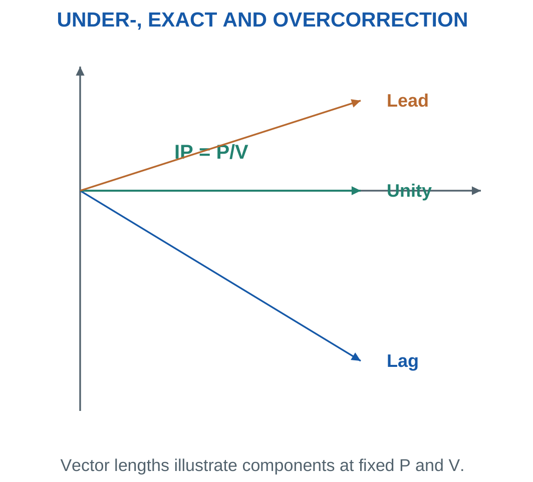
At fixed active power and voltage, source current is minimum when net reactive power is zero.
Adding capacitance beyond that point makes net Q negative. Source power factor becomes leading, and source-current magnitude begins increasing again.

For an installed capacitor:
Qc = 2πfCV²
Calculate actual compensation before finding net Q.
Changes in frequency, voltage or load condition change the final power factor. At fixed f and C, multiplying voltage by k multiplies capacitor reactive power by k².
For a desired leading target, Qtarget is negative. The general compensation equation is:
Qc = Qload − Qtarget
This requires more compensation than unity correction when the original load is inductive.
A capacitor sized for one operating point may overcorrect after the inductive load decreases. Recalculate active and reactive powers rather than assuming the original final PF remains valid.
Worked Problem 2.78: Check an Installed Capacitor
Problem: P = 1200 W, Qload = 900 var, V = 200 V, f = 50 Hz and C = 100 μF.
Qc = 2π × 50 × 100 × 10⁻⁶ × 200².
Qc = 1256.64 var.
Net Q:
Qnet = 900 − 1256.64.
Qnet = −356.637 var.
S = √(1200² + 356.637²).
S = 1251.87 VA.
I = S/200.
I = 6.25937 A.
PF = 0.958562 leading.
The unity-PF minimum current at the same P and V is 1200/200 = 6 A.
Worked Problem 2.79: Overcorrection at 230 V
Problem: P = 2000 W, Qload = 1500 var, V = 230 V, f = 50 Hz and C = 150 μF.
Capacitor compensation:
Qc = 2492.85 var.
Net reactive power:
Qnet = −992.854 var.
Apparent power:
S = 2232.88 VA.
Source current:
I = 9.70818 A.
Power factor:
PF = 0.895704 leading.
The minimum possible source current for the same active power and voltage is 8.69565 A. The excess leading component keeps actual current above that minimum.
Worked Problem 2.80: A Larger Capacitor at 100 V
Problem: P = 600 W, Qload = 800 var, V = 100 V, f = 50 Hz and C = 400 μF.
Qc = 2πfCV².
Qc = 1256.64 var.
Qnet = 800 − 1256.64.
Qnet = −456.637 var.
S = √(600² + 456.637²).
S = 754.001 VA.
I = S/100.
I = 7.54001 A.
PF = 0.795755 leading.
Unity-PF current would be 6 A. More capacitance is therefore not always better.
Worked Problem 2.81: Partial Correction Remains Lagging
Problem: P = 1000 W, Qload = 750 var, V = 200 V, f = 60 Hz and C = 40 μF.
Qc = 2π × 60 × 40 × 10⁻⁶ × 200².
Qc = 603.186 var.
Qnet = 750 − 603.186.
Qnet = 146.814 var.
S = √(1000² + 146.814²).
S = 1010.72 VA.
I = S/200.
I = 5.0536 A.
PF = 0.989394 lagging.
The capacitor improves PF substantially without crossing into leading operation.
26. Current, Line Loss and Energy After Correction
For fixed load active power P and voltage V:
I1 = P/(VPF1)
I2 = P/(VPF2)
Therefore:
I2/I1 = PF1/PF2
Current percentage reduction is:
100[1 − PF1/PF2]
For unchanged line resistance:
Ploss = I²Rline
Thus:
Ploss,2/Ploss,1 = (I2/I1)²
Absolute loss reduction is:
ΔPloss = (I1² − I2²)Rline

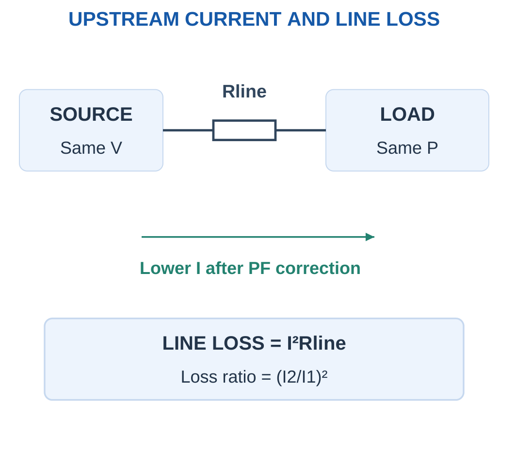
If the reduction continues for t hours:
Energy saved = ΔPloss × t/1000 kWh
when ΔPloss is in watts.
A decrease in apparent power is not automatically an equal decrease in active load power.
These comparisons hold useful load power and terminal voltage fixed and neglect capacitor losses. If upstream voltage drop changes the operating point significantly, the complete network must be analysed.
Worked Problem 2.82: Current and Line-Energy Saving
Problem: A 2000 W load at 230 V improves from PF 0.6 to 0.95. Total path resistance is 0.4 Ω. Find savings over eight hours.
I1 = 2000/(230 × 0.6).
I1 = 14.4928 A.
I2 = 2000/(230 × 0.95).
I2 = 9.15332 A.
Current reduction:
5.33944 A or 36.8421%.
Initial line loss:
84.016 W.
Corrected line loss:
33.5133 W.
Loss reduction:
50.5027 W.
Energy saved:
50.5027 × 8/1000.
0.404021 kWh.
The useful load still consumes 2000 W in the assumed comparison.
Worked Problem 2.83: Unity Correction of a 5 kW Load
Problem: P = 5000 W, V = 250 V, PF changes from 0.75 to unity and path resistance is 0.2 Ω. Operation lasts six hours.
Initial current:
I1 = 26.6667 A.
Corrected current:
I2 = 20 A.
Current reduction:
6.66667 A or 25%.
Initial loss:
I1² × 0.2.
142.222 W.
Corrected loss:
20² × 0.2.
80 W.
Loss reduction:
62.2222 W.
Energy saved:
62.2222 × 6/1000.
0.373333 kWh.
Worked Problem 2.84: A Low Initial Power Factor
Problem: P = 1200 W, V = 120 V, PF improves from 0.5 to 0.9 and path resistance is 0.15 Ω. Operation lasts ten hours.
Initial current:
I1 = 20 A.
Corrected current:
I2 = 11.1111 A.
Current reduction:
8.88889 A or 44.4444%.
Initial path loss:
60 W.
Corrected path loss:
18.5185 W.
Loss reduction:
41.4815 W.
Energy saved:
0.414815 kWh.
The benefit applies to the stated upstream loss boundary, not to an assumed reduction of useful active load power.
27. Single-Phase Wattmeter: Connection and Principle
A wattmeter measures average active power by combining voltage and current information.
Its current coil, CC, is connected in series with the measured load path.
Its pressure coil or voltage coil, PC, is connected across the load terminals in the ideal arrangement used here.

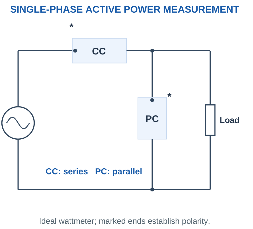
The ideal instrument averages:
v(t)i(t)
For sinusoidal operation:
W = VI cos φ
It therefore reads watts rather than simply volt-amperes.
Marked terminals establish reference polarity. Reversing only one of the voltage or current references reverses the indicated sign. Reversing both preserves the sign.
The current coil is modelled as a low-resistance series element. The pressure coil is a high-resistance shunt element.
Swapping their roles is not another valid ideal connection.
Ideal Measurement Assumptions
The numerical examples assume zero current-coil resistance and negligible pressure-coil current.
If coil resistance or coil consumption is supplied, include the specified loading correction.
A wattmeter’s reading alone does not reveal leading or lagging phase because cosine has the same value for equal positive and negative angles.
Worked Problem 2.85: Wattmeter Reading of an RL Load
Problem: V = 230 V, I = 5 A and PF = 0.8 for an RL load.
Apparent power:
S = 1150 VA.
Wattmeter reading:
W = 230 × 5 × 0.8.
W = 920 W.
Reactive-power magnitude:
√(1150² − 920²).
Q = +690 var.
Phase magnitude:
36.8699°.
The RL description establishes lagging behaviour. The positive wattmeter reading alone would not establish that direction.
Worked Problem 2.86: Wattmeter Reading of an RC Load
Problem: V = 120 V, I = 4 A and PF = 0.6 for an RC load.
S = 120 × 4.
S = 480 VA.
W = 120 × 4 × 0.6.
W = 288 W.
Reactive-power magnitude is 384 var.
For the stated capacitive model:
Q = −384 var.
Current leads by 53.1301°.
The meter still reads positive active power because the positive resistor absorbs average energy.
Worked Problem 2.87: A 0.75 PF RL Load
Problem: V = 100 V, I = 2 A and PF = 0.75.
S = 200 VA.
W = 100 × 2 × 0.75.
W = 150 W.
Reactive power:
Q = √(200² − 150²).
Q = +132.288 var.
Phase magnitude:
41.4096°.
The wattmeter reading is lower than apparent power because current contains a reactive component.
28. Identifying a Load from V, I and W
A voltmeter, ammeter and wattmeter together provide:
S = VI
P = W
PF = W/(VI)
Then:
|φ| = cos⁻¹(PF)
Reactive-power magnitude is:
|Q| = √[(VI)² − W²]

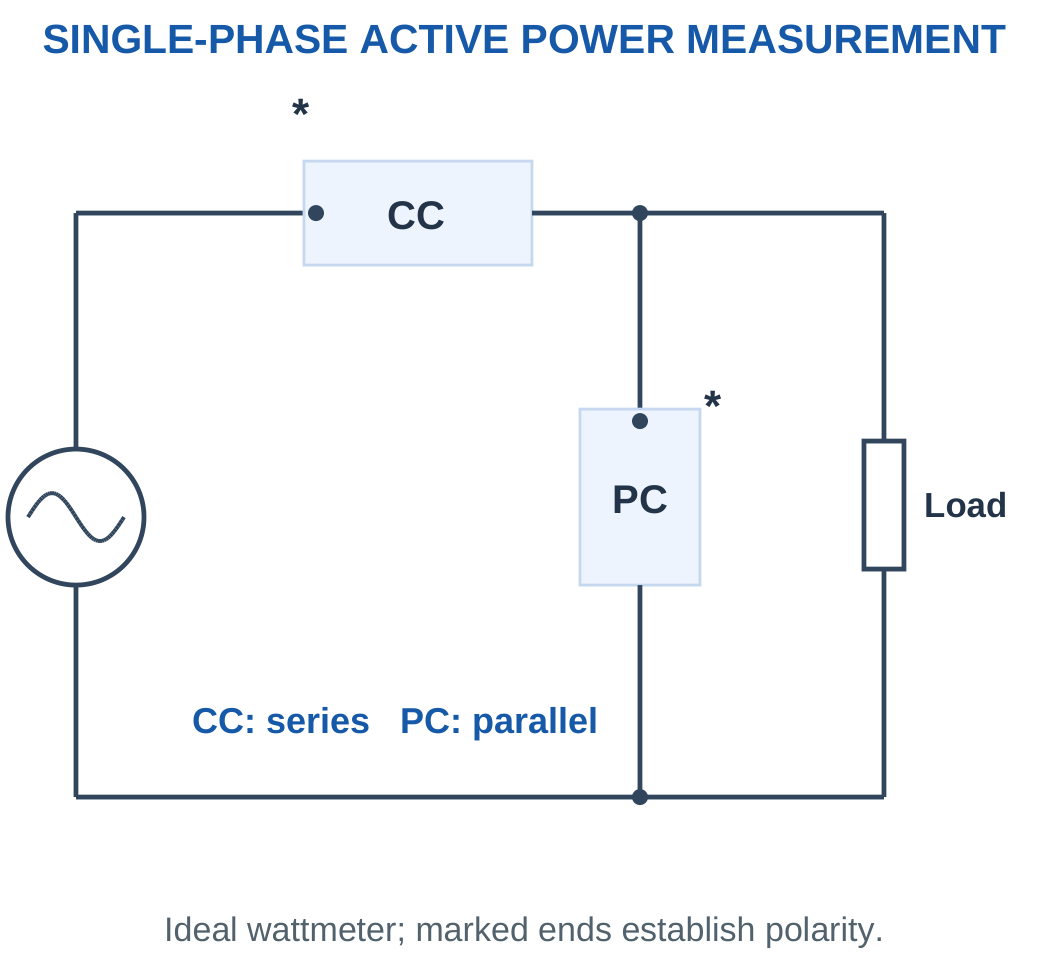
For a stated series RL load:
R = W/I²
|Z| = V/I
XL = √(|Z|² − R²)
L = XL/(2πf)
For a stated series RC load, recover XC similarly and use:
C = 1/(2πfXC)
Physical Bounds
For passive sinusoidal data:
0 ≤ W ≤ VI
If W exceeds VI, calculated PF exceeds unity and the supplied measurements are inconsistent with the assumed model.
Check instrument scale, RMS versus peak values and numerical transcription.
Rounded measurements should not be reported as derived component values with unjustified precision. The displayed worked results use the stated inputs and rounded final values.
Worked Problem 2.88: Identify a Series RL Load
Problem: V = 100 V RMS, I = 2 A RMS, W = 120 W and f = 50 Hz.
S = 200 VA.
PF = 120/200.
PF = 0.6 lagging.
|Z| = 100/2.
|Z| = 50 Ω.
R = 120/4.
R = 30 Ω.
XL = √(50² − 30²).
XL = 40 Ω.
L = 0.127324 H.
Q = +160 var.
Current phase is −53.1301° relative to voltage.
Worked Problem 2.89: Identify a Series RC Load
Problem: V = 200 V, I = 4 A, W = 640 W and f = 50 Hz.
S = 800 VA.
PF = 0.8 leading.
|Z| = 200/4.
|Z| = 50 Ω.
R = 640/16.
R = 40 Ω.
XC = √(50² − 40²).
XC = 30 Ω.
C = 1/(2π × 50 × 30).
C = 106.103 μF.
Q = −480 var.
Current leads voltage by 36.8699°.
Worked Problem 2.90: Identify a 60 Hz RL Load
Problem: V = 120 V, I = 3 A, W = 216 W and f = 60 Hz.
S = 360 VA.
PF = 0.6 lagging.
|Z| = 120/3.
|Z| = 40 Ω.
R = 216/9.
R = 24 Ω.
XL = √(40² − 24²).
XL = 32 Ω.
L = 0.0848826 H.
Q = +288 var.
The current angle is −53.1301° with voltage as reference.
Worked Problem 2.91: Identify a 230 V RC Load
Problem: V = 230 V, I = 5 A, W = 690 W and f = 50 Hz.
S = 1150 VA.
PF = 0.6 leading.
|Z| = 230/5.
|Z| = 46 Ω.
R = 690/25.
R = 27.6 Ω.
XC = √(46² − 27.6²).
XC = 36.8 Ω.
Capacitance:
C = 86.4973 μF.
Reactive power:
Q = −920 var.
The RC description provides the leading direction that the three magnitude readings alone cannot supply.
29. Wattmeter Range, Scale and Reading Checks
Suppose a wattmeter has selected voltage range Vrange, current range Irange and D equal divisions.
Under the stated full-scale range-product model:
Full-scale watts = VrangeIrange
Scale constant:
K = VrangeIrange/D watts per division
For deflection d:
W = Kd

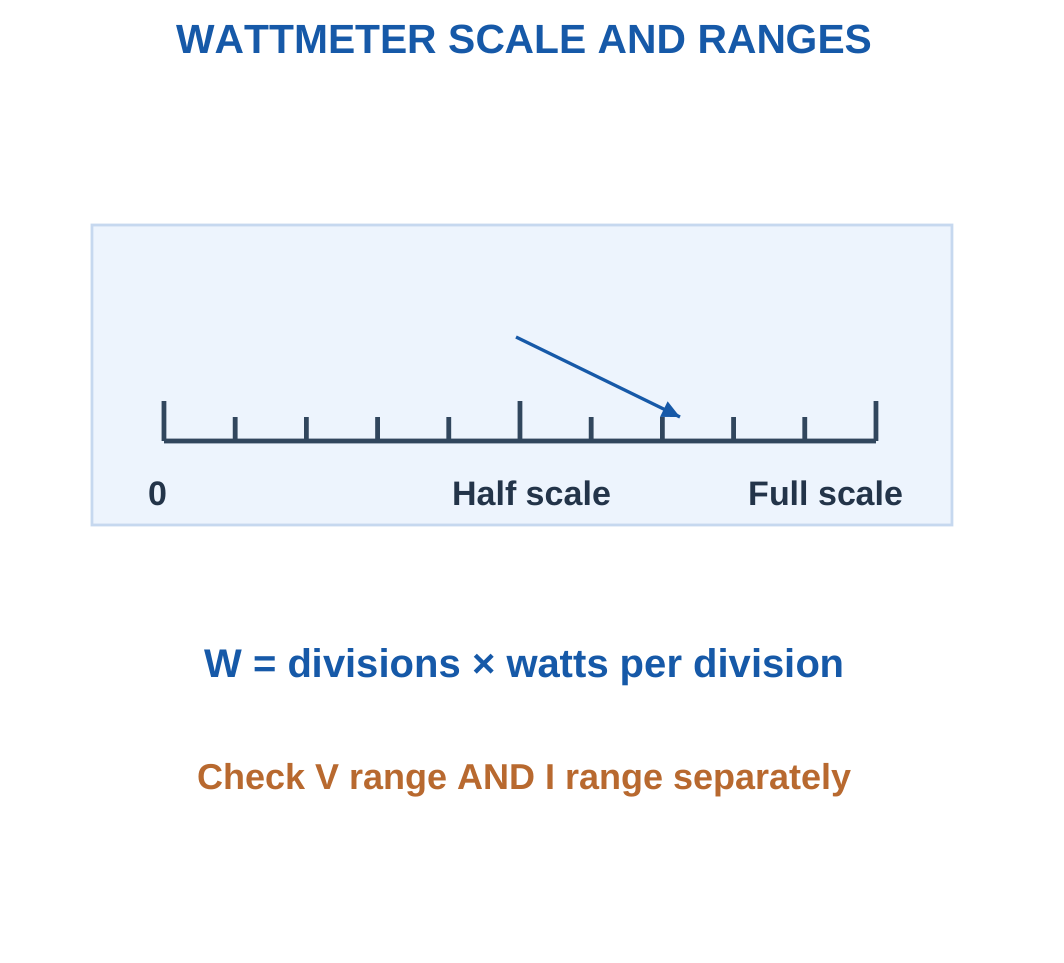
If the problem gives an independent multiplying factor or explicit full-scale watt value, use that supplied information instead of assuming the range product.
A low-power-factor load may give a small watt reading while current is large. Therefore checking only watts against full-scale watts is insufficient.
Both selected coil limits must pass:
Vactual ≤ Vrange
Iactual ≤ Irange
A negative reading can indicate reversed reference polarity or actual reverse active-power flow. Interpret the circuit before replacing the sign with a magnitude.
Worked Problem 2.92: Scale Conversion and Range Check
Problem: Ranges are 300 V and 5 A, with 150 divisions. Deflection is 92 divisions. Separate readings are 230 V and 5 A.
Full-scale power:
300 × 5.
1500 W.
Scale constant:
1500/150.
10 W per division.
Indicated power:
92 × 10.
W = 920 W.
Apparent power:
230 × 5.
S = 1150 VA.
PF = 920/1150.
PF = 0.8.
Voltage is within 300 V. Current equals the selected 5 A limit. Both ideal range checks pass.
Wattmeter Connection Context

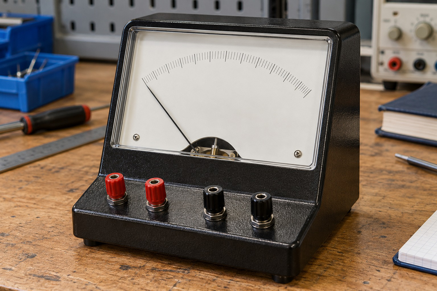
A wattmeter combines current and voltage measurement functions. Coil connections, polarity and selected ranges determine interpretation.
The algebraic sign matters whenever readings are compared or combined. A scale magnitude by itself is not a complete description of the measured power reference.
Worked Problem 2.93: Physically Inconsistent Power-Factor Data
Problem: Ranges are 300 V and 10 A with 150 divisions. Deflection is 120 divisions. Separate readings are 250 V and 8 A.
Full-scale watts:
300 × 10.
3000 W.
Scale constant:
3000/150.
20 W per division.
Indicated power:
120 × 20.
W = 2400 W.
Apparent power:
250 × 8.
S = 2000 VA.
Calculated PF:
2400/2000.
PF = 1.2.
This is inconsistent with the assumed passive sinusoidal measurements.
Both coil ranges pass, but range validity does not make the incompatible numerical readings physically consistent.
Worked Problem 2.94: Current Range Exceeded
Problem: Ranges are 150 V and 5 A with 75 divisions. Deflection is 48 divisions. Separate readings are 100 V and 6 A.
Full-scale watts:
150 × 5.
750 W.
Scale constant:
750/75.
10 W per division.
Indicated power:
48 × 10.
W = 480 W.
Apparent power:
100 × 6.
S = 600 VA.
Calculated PF:
0.8.
Voltage range passes, but:
6 A > 5 A.
The current range is exceeded. The setup fails its range check despite a plausible PF and a scale indication below full scale.
30. Integrated AC Circuit Solutions
A complete AC solution connects waveform information, impedance, current, component voltages and power.
Start by identifying whether the circuit is series or parallel. Series elements share current. Parallel branches share voltage.
Select a reference phasor and retain it throughout the calculation.


Recommended Examination Layout
Write the given quantities with units. Convert peak values to RMS before using RMS power formulas.
Calculate angular frequency and reactance. Form complex impedance before calculating current.
State current magnitude and whether it leads or lags.
Calculate component voltages using the common current. Reconstruct supply voltage by phasor addition.
Calculate P, Q, S and PF. Interpret reactive-power sign.
For correction questions, analyse the original load first and then add signed capacitor reactive power at the same terminal voltage.
Choose an Efficient Starting Point
If R and L or C are supplied, start with impedance.
If V, I and W are supplied, start with S, PF and resistance.
If P and PF are supplied, calculate Q using P tan φ.
Each route should produce compatible physical results. A numerical magnitude without lead or lag information is incomplete when phase is part of the requested answer.
Worked Problem 2.95: Integrated RL Calculation

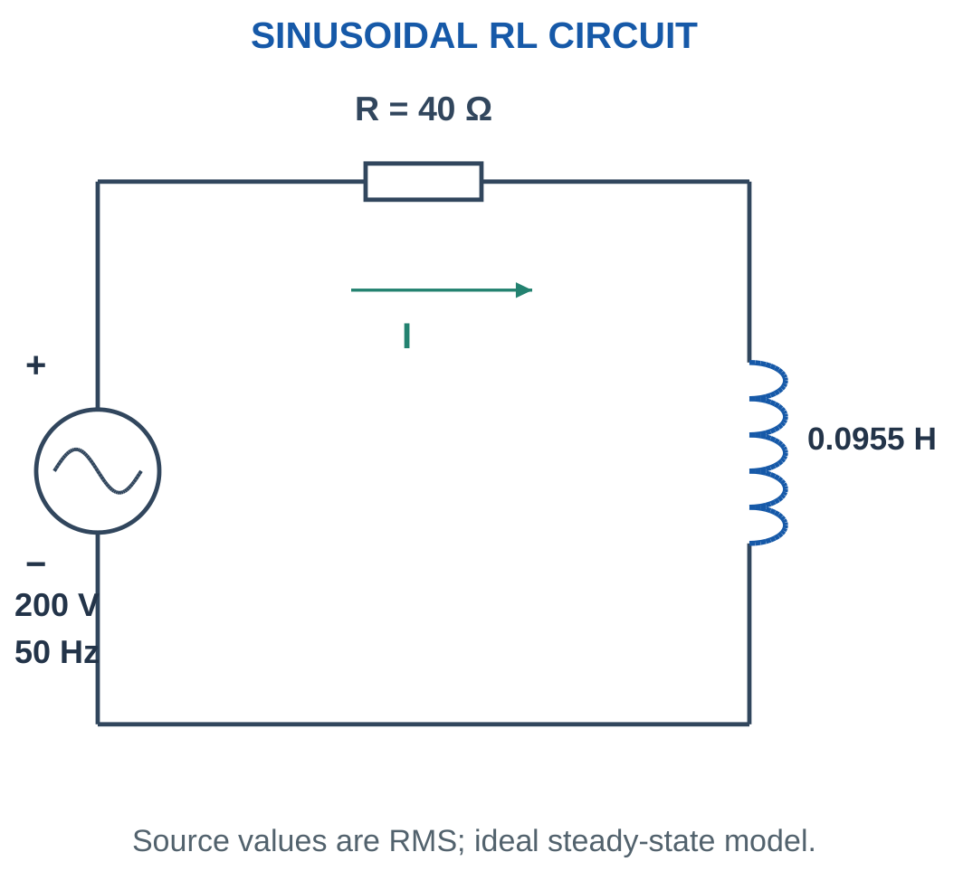
Problem: R = 40 Ω and L = 0.095493 H.
XL = 2π × 50 × 0.095493.
XL ≈ 30 Ω.
Z = 40 + j30 Ω.
|Z| = 50 Ω.
Impedance angle:
36.8699°.
Current:
I = 4 A at −36.8699°.
Component drops:
VR = 160 V.
VL = 120 V.
Power:
P = 640 W.
Q = +480 var.
S = 800 VA.
PF = 0.8 lagging.
Current waveform:
i = 5.65685 sin(314.159t − 0.643501) A
Worked Problem 2.96: Integrated RL Calculation at 60 Hz
Problem: R = 30 Ω, L = 0.106103 H, V = 150 V RMS and f = 60 Hz.
XL ≈ 40 Ω.
Z = 30 + j40 Ω.
|Z| = 50 Ω.
Current:
I = 3 A lagging by 53.1301°.
Resistor voltage:
VR = 90 V.
Inductor voltage:
VL = 120 V.
Power quantities:
P = 270 W.
Q = +360 var.
S = 450 VA.
PF = 0.6 lagging.
Current waveform:
i = 4.24264 sin(376.991t − 0.927295) A
The voltage triangle gives √(90² + 120²) = 150 V.
Worked Problem 2.97: Integrated RC Calculation


Problem: R = 40 Ω and C = 106.103 μF.
XC ≈ 30 Ω.
Z = 40 − j30 Ω.
|Z| = 50 Ω.
Impedance angle:
−36.8699°.
Current:
I = 4 A leading by 36.8699°.
Component voltages:
VR = 160 V.
VC = 120 V.
Power quantities:
P = 640 W.
Q = −480 var.
S = 800 VA.
PF = 0.8 leading.
Current waveform:
i = 5.65685 sin(314.159t + 0.643501) A
The RL and RC examples can have identical current magnitude, active power and apparent power while differing in phase direction and reactive-power sign.
31. Examination Techniques and Error Diagnosis
Check the Type of Electrical Value
Distinguish instantaneous, peak, peak-to-peak, RMS and rectified average values.
For a sine wave:
Rectified average < RMS < Peak
A phase shift does not change any of these magnitude measures. It changes the waveform timing relative to the reference.
Do not divide an arbitrary instantaneous sample by √2 and call the result RMS.
Check Reactance Before Impedance
Inductance in henries is not reactance in ohms.
Capacitance in farads is not reactance in ohms.
Calculate XL or XC using the actual frequency before forming impedance.
Use the positive reactance magnitude and then attach the correct imaginary sign: positive for inductive and negative for capacitive impedance.
Check Current Direction in the Phasor Diagram
When supply voltage is zero phase, current angle is the negative of impedance angle.
Positive inductive impedance angle gives negative current phase.
Negative capacitive impedance angle gives positive current phase.
A correct magnitude with the wrong phase direction gives the wrong reactive-power sign.
Check Voltage Addition
The supply in a series RL or RC circuit is the vector sum of component voltages.
Do not add resistor and reactive voltage magnitudes arithmetically.
Use the Pythagorean relation only when the relevant phasors are perpendicular. For arbitrary phase separation, use rectangular addition or the general cosine expression.
Check Power in Two Ways
Once current is known, calculate:
P = I²R
Then independently calculate:
P = VI cos φ
Agreement checks the current, resistance, phase magnitude and RMS convention.
Similarly compare:
S = VI
with:
S = √(P² + Q²)
A passive-series circuit with a calculated current larger than V/R may indicate that reactance was incorrectly subtracted from resistance as an ordinary scalar.
Check Correction Using Signed Reactive Power
For a shunt capacitor, source active power remains unchanged in the ideal fixed-voltage model.
Subtract compensation from inductive Q, then calculate the new current magnitude.
Do not subtract current magnitudes directly.
If net Q becomes negative, report leading PF. A decimal without its direction omits an essential part of the result.
Check Instrument Data
A PF above unity indicates incompatible data under the passive sinusoidal model.
Possible causes include a missed scale constant, peak and RMS values being mixed, incorrect current or voltage units, or a transcription error.
Check each wattmeter coil range separately. A low active-power reading does not establish that the current coil is within range.
Rounding Practice
Retain useful intermediate precision, particularly in reactance, phase and compensation calculations.
Round final results to a sensible precision and include the appropriate unit.
A result can pass a dimensional check while still failing a topology or phase check. Verification should include both arithmetic and physical interpretation.
32. Formula Sheet with Conditions
| Quantity | Formula | Condition |
|---|---|---|
| Sinusoidal voltage | v = Vm sin(ωt + θ) | State peak amplitude and reference |
| Angular frequency | ω = 2πf | f in hertz |
| Period | T = 1/f | One complete cycle |
| Phase from delay | Δθ = 360fΔt | Δt in seconds |
| Sinusoidal RMS | V = Vm/√2 | Sine wave |
| Current RMS | I = Im/√2 | Sine wave |
| Rectified average | Vavg = 2Vm/π | Full-wave rectified or positive half-cycle |
| Signed average | Zero | Symmetrical sine over full cycle |
| Form factor | π/(2√2) | Sine wave |
| Crest factor | √2 | Sine wave |
| Inductive reactance | XL = 2πfL | L in henries |
| Capacitive reactance | XC = 1/(2πfC) | C in farads |
| Inductive impedance | jXL | Positive XL magnitude |
| Capacitive impedance | −jXC | Positive XC magnitude |
| Series RL | Z = R + jXL | Common current |
| Series RC | Z = R − jXC | Common current |
| Impedance magnitude | √(R² + X²) | One series R and reactive component |
| RMS current | I = V/ | Z |
| RL phase | tan⁻¹(XL/R) | Current lags |
| RC phase magnitude | tan⁻¹(XC/R) | Current leads |
| Series voltage triangle | V² = VR² + VX² | Quadrature component drops |
| Active power | P = VI cos φ | RMS quantities |
| Peak-value active power | P = VmIm cos φ/2 | Peak quantities |
| Reactive power | Q = VI sin φ | Signed φ |
| Apparent power | S = VI | RMS magnitude product |
| Complex power | VI* = P + jQ | Conjugate current |
| Power triangle | S² = P² + Q² | Sinusoidal steady state |
| Power factor | PF = P/S | State leading or lagging |
| Series resistor power | P = I²R | Actual branch current |
| Inductor energy | w = Li²/2 | Instantaneous current |
| Capacitor energy | w = Cv²/2 | Instantaneous voltage |
| Capacitor compensation | Qc = ωCV² | Single-phase shunt capacitor |
| Correction size | Qc = Qload − Qtarget | Signed target Q |
| Lagging-to-less-lagging correction | Qc = P(tan φ1 − tan φ2) | Fixed P |
| Correction capacitance | C = Qc/(2πfV²) | RMS capacitor voltage |
| Source current from P and PF | I = P/(VPF) | Sinusoidal load |
| Line loss | I²Rline | Specified resistance boundary |
| Wattmeter | W = VI cos φ | Ideal sinusoidal measurement |
| Scale constant | K = Full-scale watts / Divisions | Use supplied calibration |
| Energy | Wenergy = Pt | Constant active power |
Formula Conditions
A correct expression applied under the wrong assumptions still produces an incorrect answer.
All phasors in one calculation must have the same frequency and magnitude convention.
The source voltage and current used in power calculation must refer to the same load boundary.
Capacitor-correction voltage is the RMS voltage across that capacitor.
The familiar tangent-difference expression assumes an initially lagging load and a lagging or unity target. A leading target requires signed reactive-power treatment.
33. Short-Answer Questions with Clear Answers
1. Why Is RMS Called the Effective Value?
Answer: RMS gives the DC value that produces the same average heating in a specified ideal resistor.
The comparison depends on the average of i²R. Negative current values still produce positive resistor heating because current is squared.
RMS is therefore not the signed average of current. A symmetrical sine has zero signed average but nonzero RMS value.
2. Is the Average Value of a Sine Wave Zero?
Answer: The signed average over one complete symmetrical cycle is zero because positive and negative areas cancel.
The positive half-cycle average and full-wave rectified average are both 2Vm/π.
State the interval and operation before giving an average value. Without that qualification, the word average can refer to two different quantities.
3. Why Does Inductor Current Lag Voltage?
Answer: The inductor relationship is v = L di/dt.
For sinusoidal current, differentiation advances the waveform by 90°. Voltage therefore leads current by one quarter-cycle.
Current reaches its maximum when ideal inductor voltage is zero. Voltage is greatest when current is changing most rapidly.
4. Why Does Capacitor Current Lead Voltage?
Answer: Capacitor current is i = C dv/dt.
It depends on the slope of voltage rather than voltage alone.
Current magnitude is greatest at a voltage zero crossing and zero at a voltage peak. For a sinusoidal waveform, this produces a 90° current lead in an ideal capacitor.
5. Can a Pure Inductor Draw Current but No Watts?
Answer: Yes.
An ideal inductor alternately stores magnetic energy and returns it to the source. Positive and negative instantaneous energy transfers cancel over a complete cycle.
Its average active power is zero, while RMS current, apparent power and reactive power can all be nonzero.
6. Why Are RL Voltages Not Added Arithmetically?
Answer: Resistor voltage and ideal inductor voltage are 90° apart when expressed relative to their common current.
Their phasors add, while their magnitudes satisfy:
V = √(VR² + VL²)
Their instantaneous signed values still satisfy KVL at every instant.
7. What Does Negative Reactive Power Mean?
Answer: Under the passive convention used here, negative Q represents capacitive reactive behaviour.
It corresponds to current leading voltage.
It does not by itself mean negative average active power. A series RC load can absorb positive watts while having negative reactive power.
8. Does PF = 0.8 Identify Leading or Lagging Operation?
Answer: No.
The cosine has the same value for positive and negative phase angles of equal magnitude.
A circuit description, phase observation or another suitable datum is required to identify direction. Report 0.8 lagging for an inductive load or 0.8 leading for a capacitive load when that information is available.
9. Why Is a Correction Capacitor Connected in Parallel?
Answer: A shunt capacitor draws leading current at the same load-terminal voltage.
In the ideal analysis, the original load remains connected to the same voltage and retains its original branch behaviour.
The capacitor modifies the combined source current rather than becoming a series part of the original load.
10. Does Unity Source PF Mean Zero Capacitor Current?
Answer: No.
The capacitor current can cancel the inductive reactive component at the source while remaining nonzero in its own branch.
Unity source PF means net source reactive power is zero. It does not imply that every reactive branch has zero current or zero stored energy.
11. Why Does Overcorrection Increase Source Current?
Answer: Current is minimum at zero net reactive power for fixed active power and voltage.
Beyond that point, additional capacitance creates a leading reactive component.
The active component remains fixed, while the growing perpendicular component increases the magnitude of the source-current vector.
12. Can a Wattmeter Alone Identify Leading Power Factor?
Answer: No.
The ideal reading is VI cos φ. Equal positive and negative phase angles give the same reading.
A wattmeter provides active power relative to its marked references. Additional phase or circuit information is required to identify whether current leads or lags voltage.
13. Why Is a Low Watt Reading Not Proof of an Acceptable Current Range?
Answer: At low power factor, VI can be large while VI cos φ is small.
A current coil can therefore carry more than its selected range even when the indicated watts are relatively low.
Check actual voltage and current against their individual selected ranges independently.
14. Is 50 Hz the Same as 50 rad/s?
Answer: No.
At 50 Hz:
ω = 2π × 50 = 100π rad/s
Therefore:
ω ≈ 314.159 rad/s
Hertz counts complete cycles each second. Angular frequency counts radians each second. One cycle contains 2π radians.
15. Does the Sine-Wave RMS Factor Apply to Every Waveform?
Answer: No.
The factor 1/√2 follows from the average of sin² being one half.
For another waveform, calculate the mean square from its actual shape or supplied samples. Unequal sample durations require time weighting rather than an unweighted arithmetic mean.
34. Complete Examination Answers
1. Derive the RMS Value of a Sinusoidal Voltage
Answer:
Let:
v = Vm sin ωt
and let T be one complete period.
By definition:
Vrms² = (1/T)∫₀ᵀv²dt
Substitute the sinusoidal equation:
Vrms² = (Vm²/T)∫₀ᵀsin²ωt dt.
Use:
sin²α = (1 − cos 2α)/2
Therefore:
Vrms² = (Vm²/2T)∫₀ᵀ(1 − cos 2ωt)dt.
Over one complete period, the cosine term integrates to zero. The remaining integral is T.
Hence:
Vrms² = Vm²/2
Taking the positive square root:
Vrms = Vm/√2
The same derivation gives:
Irms = Im/√2
For a resistor, average heating is Irms²R. A DC current equal to Irms produces the same average heating in that resistor.
The derivation is specific to a sinusoid. The general RMS definition must be used for other waveform shapes.
2. Derive Average Value and Form Factor
Answer:
For a positive half-cycle:
v = Vm sin θ
The angular interval extends from zero to π radians.
Average value is:
Vavg = (1/π)∫₀ᵖⁱVm sin θ dθ
Integrating:
Vavg = (Vm/π)[−cos θ]₀ᵖⁱ.
At θ = π, cosine is −1. At θ = 0, cosine is +1.
Therefore:
Vavg = 2Vm/π
Numerically:
Vavg ≈ 0.6366Vm
The full-wave rectified average is the same because the negative half-cycle is reflected upward.
The signed full-cycle average remains zero.
Form factor is RMS divided by rectified average:
Form factor = (Vm/√2)/(2Vm/π).
Therefore:
Form factor = π/(2√2)
Form factor ≈ 1.1107
Crest factor is peak divided by RMS:
Crest factor = √2 ≈ 1.4142
Both factors are dimensionless and independent of amplitude for a sine wave.
3. Explain a Series RL Circuit Using Phasors
Answer:
A series RL circuit carries the same current through the resistor and ideal inductor.
Choose current as the reference phasor.
Resistor voltage is:
VR = IR
and is in phase with current.
Inductor voltage is:
VL = IXL
and leads current by 90°.
KVL gives:
V = VR + jVL.
Therefore:
V = I(R + jXL)
The impedance is:
Z = R + jXL
Its magnitude is:
|Z| = √(R² + XL²)
The impedance angle is:
φ = tan⁻¹(XL/R)
Current magnitude is V/|Z|. When supply voltage is the zero-degree reference, current angle is −φ, so current lags.
Power factor is R/|Z|.
Active power is I²R. Reactive power is positive I²XL.
The voltage triangle gives:
V² = VR² + VL²
The ideal inductor stores and returns magnetic energy but has no average active dissipation.
A complete answer identifies the reference, constructs impedance, calculates current and checks voltage and power relationships.
4. Explain a Series RC Circuit Using Phasors
Answer:
A series RC circuit carries common current through the resistor and capacitor.
Choose current as reference.
Resistor voltage is IR and lies on the positive real axis. Capacitor voltage has magnitude IXC and lags current by 90°, so it points down the imaginary axis.
KVL gives:
V = I(R − jXC)
Therefore:
Z = R − jXC
Its magnitude is:
|Z| = √(R² + XC²)
Its angle is negative:
θZ = −tan⁻¹(XC/R)
For supply voltage at zero degrees, current angle is −θZ and is positive. Thus current leads supply voltage.
Power factor is R/|Z| leading.
Active power is I²R.
Reactive power is:
Q = −I²XC
Apparent power is VI.
Component-voltage magnitudes satisfy:
V² = VR² + VC²
The capacitor’s current lead relative to its own voltage is 90°, while the current lead relative to the complete supply is generally smaller when resistance is nonzero.
This distinction prevents confusion between a pure capacitor and a series RC branch.
5. Explain the Power Triangle and Complex Power
Answer:
For RMS phasors:
Scomplex = VI = P + jQ*
The current is conjugated so that the standard passive-load reactive-power sign is obtained.
The real component is:
P = VI cos φ
measured in watts.
The imaginary component is:
Q = VI sin φ
measured in var.
The magnitude is:
S = VI
measured in VA.
The power triangle places P horizontally and signed Q vertically. Apparent power is the hypotenuse.
Therefore:
S² = P² + Q²
and:
PF = P/S
For positive active power:
tan φ = Q/P
Inductive Q is positive. Capacitive Q is negative.
A negative Q changes the triangle direction but does not imply negative P.
For combined loads, add P values and signed Q values separately. Then find the magnitude of the resulting complex power.
Adding apparent-power magnitudes is valid only under the appropriate common-angle condition. In general, it ignores the phase relationship between load currents.
6. Derive the Shunt Capacitor Correction Formula
Answer:
Consider an inductive load with active power P at unchanged terminal RMS voltage V.
Initial power factor is cos φ1, so:
Q1 = P tan φ1
The desired lagging target has:
Q2 = P tan φ2
A shunt capacitor supplies negative reactive power. If Qc denotes its positive compensation size:
Q2 = Q1 − Qc.
Therefore:
Qc = P(tan φ1 − tan φ2)
An ideal capacitor across RMS voltage V draws:
Ic = ωCV
Its reactive-power magnitude is:
Qc = VIc.
Therefore:
Qc = ωCV²
Hence:
C = P(tan φ1 − tan φ2)/(ωV²)
Using ω = 2πf:
C = P(tan φ1 − tan φ2)/(2πfV²)
At unity target power factor, φ2 = 0 and Qc equals the original inductive reactive power.
Load active power remains unchanged in the ideal fixed-voltage comparison. Source current falls because the net reactive component decreases.
For a leading target, use signed Qtarget in the general equation rather than treating both tangent terms as positive lagging quantities.
7. Explain Single-Phase Wattmeter Power Measurement
Answer:
A single-phase wattmeter combines a current-dependent signal and a voltage-dependent signal.
The current coil is connected in series with the load path. The pressure coil is connected across the load terminals.
In the ideal model, the instrument averages the instantaneous product:
p(t) = v(t)i(t)
For sinusoidal voltage and current:
W = VI cos φ
The reading is active power in watts.
The instrument therefore accounts for phase displacement. Multiplying separate voltmeter and ammeter readings gives apparent power, not generally the wattmeter reading.
Marked coil terminals establish reference polarity. Reversing one reference reverses the indicated power sign. Reversing both leaves the sign unchanged.
With separate V and I readings:
PF = W/(VI)
Reactive-power magnitude is:
|Q| = √[(VI)² − W²]
Leading or lagging direction requires additional information because cosine does not distinguish equal positive and negative angles.
Check both voltage and current ranges separately. A low-power-factor load may produce a low watt indication while carrying a large current.
Use the supplied scale constant or multiplying factor when converting a deflection into watts.
8. Explain Why Power-Factor Improvement Reduces Line Loss
Answer:
For fixed load active power P and RMS voltage V:
I = P/(VPF)
Increasing power factor reduces current while retaining the stated useful active load power.
For initial and final conditions:
I2/I1 = PF1/PF2
If conductor resistance remains unchanged:
Ploss = I²Rline
Therefore:
Ploss,2/Ploss,1 = (PF1/PF2)²
The absolute reduction is:
ΔPloss = (I1² − I2²)Rline
If this reduction continues for t hours:
Energy saved = ΔPloss × t/1000 kWh
for ΔPloss in watts.
The saving belongs to the specified upstream resistance boundary.
It is incorrect to interpret the reduction in apparent power as an equal reduction in active load energy.
The derivation assumes fixed load-terminal voltage, unchanged useful active power and negligible capacitor loss.
If correction changes voltage sufficiently to alter the load operating point, the complete network must be analysed rather than relying only on this fixed-condition comparison.
Final Revision Checklist
Waveform Checks
- Identify whether each value is instantaneous, peak, RMS or average.
- Convert milliseconds to seconds before calculating phase.
- Use a common sine or cosine convention.
- Keep radians and degrees consistent.
- State the averaging interval.
- Use sine-wave conversion factors only for sinusoidal waveforms.
Phasor Checks
- Use one frequency in each phasor calculation.
- Use one magnitude convention.
- Add and subtract in rectangular form.
- Select the correct quadrant.
- Keep the common reference unchanged.
- Interpret negative angles using the selected reference.
- Do not add component magnitudes without checking phase.
Circuit Checks
- Series branches share current.
- Parallel branches share voltage.
- Inductive impedance has positive imaginary part.
- Capacitive impedance has negative imaginary part.
- RL current lags supply voltage.
- RC current leads supply voltage.
- A pure reactive element has zero mean active power.
- A practical coil may require winding resistance.
Power and Measurement Checks
- P uses watts.
- Q uses var.
- S uses VA.
- Complex power uses current conjugation.
- State leading or lagging power factor.
- Add signed reactive powers when combining loads.
- Check correction through residual Q.
- Check voltage and current coil ranges independently.
- A PF above unity signals incompatible passive sinusoidal data.
- Use actual active-power reduction when calculating energy savings.
Final Verification Habit
A complete answer identifies the circuit model and reference, writes the governing equations, substitutes consistent units and interprets the final magnitude and phase.
Verify the voltage triangle, active power and power triangle where applicable.
The purpose of the checks is to connect the numerical answer with the waveform timing and physical circuit behaviour.