University: Dr. A.P.J. Abdul Kalam Technical University, AKTU
Programme: B.Tech First Year, Semester I and Semester II
Course Codes: AEE101A / AEE201A
Branches: Common to All
Unit: I
Unit Name: Basic Electrical Quantities and DC Circuits
Introduction to Basic Electrical Quantities and DC Circuits
Electrical engineering begins with understanding how electric charge moves, how sources transfer energy and how circuit connections determine voltage and current. These ideas are used in electrical machines, electronic systems, power networks, measurement instruments, control systems and everyday electrical equipment.
A DC circuit provides a useful starting point because the steady-state examples use quantities that remain constant with time. The current direction does not alternate, the source values are specified and positive linear resistors relate voltage and current through Ohm’s law. This makes it possible to concentrate on circuit connections, reference directions, energy transfer and systematic solution methods.
The unit begins with charge, current, potential difference, EMF, resistance and conductance. It then develops series and parallel combinations, voltage and current division, electrical power, energy calculations and practical source models. Kirchhoff’s laws provide the foundation for analysing networks that cannot be solved by an immediate resistor combination.
Nodal analysis uses unknown node potentials and Kirchhoff’s Current Law. Mesh analysis uses loop-current variables and Kirchhoff’s Voltage Law. Thevenin’s theorem replaces a linear source network with a simpler two-terminal equivalent when the external load is the main quantity of interest.
The purpose of studying these methods is to calculate the requested quantities while keeping the physical meaning clear. Current is a rate of charge transfer. Voltage is a difference between two potentials. Power is the rate at which energy is transferred. A resistor absorbs energy while charge continues through the circuit.
Reading a Circuit Before Calculating
Begin every solution by identifying the source network, the external load and the terminals mentioned in the question. A diagram can be stretched or redrawn without changing the circuit when all connections are preserved. Marking each complete wire node with one label makes these relationships easier to see.
Record whether the source is ideal or includes a stated internal resistance. This distinction determines whether its terminal voltage changes when load current changes. A fixed ideal voltage source maintains its stated voltage, while a practical series-resistance model develops an internal voltage drop.
Choose references that make the equations easy to audit. A current arrow defines a positive direction for a variable; it does not predict the eventual physical direction. A voltage polarity defines an ordered difference between two points.
Keep both references unchanged during the calculation. Retain a negative result where it appears and explain its meaning after solving. Finally, check conservation of charge, potential changes around a closed path and electrical power balance.
Unit 1 Topic Map
| Topic | Main Coverage |
|---|---|
| Basic electrical quantities | Charge, current, voltage, EMF, resistance and conductance |
| Circuit connections | Nodes, branches, loops, meshes, opens and shorts |
| Resistor networks | Series, parallel and mixed combinations |
| Divider rules | Unloaded voltage divider, loaded divider and current divider |
| Power and energy | Resistor dissipation, source power, energy and running cost |
| Practical sources | Internal resistance, terminal voltage and load regulation |
| Kirchhoff’s laws | KCL, KVL and reference conventions |
| Nodal analysis | One-node, two-node and current-injection networks |
| Mesh analysis | Shared resistors, two meshes and multiple sources |
| Thevenin’s theorem | Open-circuit voltage, equivalent resistance and load calculations |
| Measurement | Voltmeter loading and ammeter burden resistance |
| Revision | Formula sheet, short answers and long answers |
Syllabus Coverage
- Electric charge and current.
- Potential difference and EMF.
- Resistance, resistivity and conductance.
- Ohm’s law.
- Series and parallel resistor combinations.
- Voltage-divider and current-divider rules.
- DC electrical power and energy.
- Kirchhoff’s Current Law.
- Kirchhoff’s Voltage Law.
- Branch-current references.
- Simple nodal analysis.
- Simple mesh analysis.
- Thevenin’s theorem and load calculations.
- Basic electrical measurement and circuit checking.
Numerical Conventions
Unless a problem states otherwise, wires and sources are ideal. Positive resistors are linear elements with constant resistance under the assumed operating conditions.
Use the supplied numerical values. Retain useful precision during the working and round the displayed result at the end. A negative answer must be interpreted against the current arrow or voltage polarity originally assigned.
Use the same element’s voltage and current when calculating its power. Do not combine source voltage with a branch current unless those quantities actually belong to the same two-terminal element.
1. Electrical Quantities and the DC Circuit Model
An electrical circuit provides connected paths through which charges can move and energy can be transferred. Sources supply or absorb energy, conductors connect components and loads convert electrical energy into forms such as heat, light or mechanical work.
Direct current means current with a fixed direction. In the steady DC examples considered here, the electrical quantities are constant. The term DC does not by itself mean that every possible waveform must be perfectly constant; the numerical model used in this unit is the steady constant-value model unless another condition is stated.

| Quantity | Symbol | SI Unit |
|---|---|---|
| Electric charge | Q | Coulomb, C |
| Electric current | I | Ampere, A |
| Potential difference | V | Volt, V |
| Electromotive force | E | Volt, V |
| Resistance | R | Ohm, Ω |
| Conductance | G | Siemens, S |
| Power | P | Watt, W |
| Energy | W or Eenergy | Joule, J |
A circuit diagram is a connection model. It is not necessarily a drawing of the physical positions of components on a table or inside an instrument. Components drawn far apart may share the same node through an ideal wire.
Ideal wires have zero resistance. Every point joined by an uninterrupted ideal conductor belongs to the same node and has the same potential. This does not imply that every point in the entire circuit has the same potential; components separate nodes by developing voltage differences.
For a complete resistive circuit, the source and the connected network determine current. A resistor does not consume charge. It converts electrical energy into heat while charge continues through the conducting path.
First Habit
Before calculating, label the requested current direction and voltage polarity. A negative answer reverses the chosen reference. It does not automatically mean an impossible circuit.
Worked Problem 1.1: Interpret a Simple DC Load
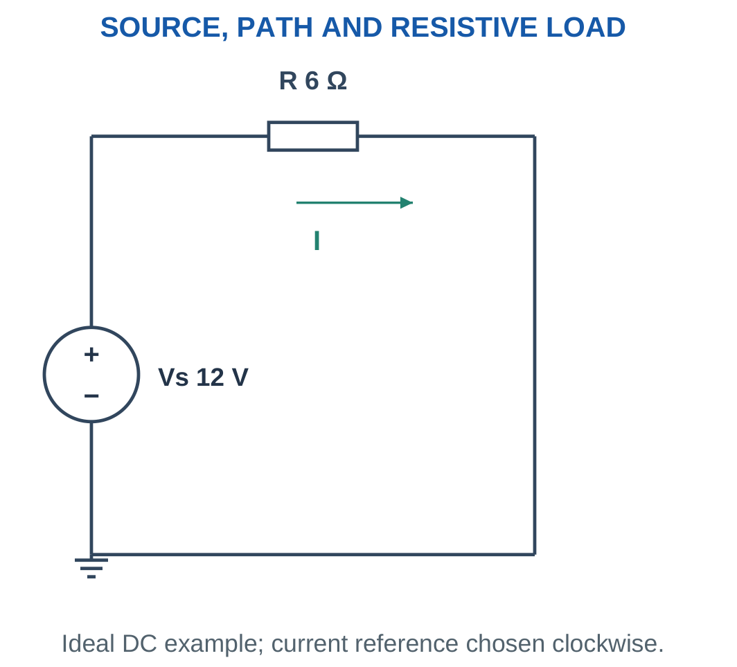
Problem: An ideal 12 V source supplies a 6 Ω resistor. Find load current and power, and identify where energy is transferred.
Step 1: Calculate current.
I = V/R
I = 12/6 = 2 A.
Step 2: Calculate load power.
Pload = VI
Pload = 12 × 2 = 24 W.
The resistor absorbs 24 W and converts electrical energy into heat. In this ideal single-load circuit, the source delivers the same 24 W.
The current remains 2 A throughout the unbranched path. The resistor does not use up current as charge passes through it.
2. Electric Charge and Conservation of Charge
Electric charge is a property of matter. The elementary charge magnitude is approximately:
e = 1.602 × 10⁻¹⁹ C
An electron carries charge −e. A collection of n electrons has signed charge:
Q = −ne
When only charge magnitude is requested:
|Q| = ne
The number of particles is positive. The negative sign belongs to the charge carried by each electron and therefore to the collection’s total signed charge.

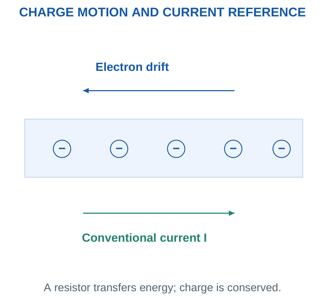
Charge is conserved. It can be transferred or redistributed, but an ordinary resistor does not destroy it. In steady operation, the charge rate entering a two-terminal resistor equals the charge rate leaving it.
This principle is the physical foundation for Kirchhoff’s Current Law. If charge were continually entering a junction faster than it left, charge would accumulate there and the steady-state model would no longer apply.
Common charge units include coulombs, millicoulombs and microcoulombs:
- 1 mC = 10⁻³ C.
- 1 µC = 10⁻⁶ C.
- 1 nC = 10⁻⁹ C.
Even a small charge measured in coulombs corresponds to a very large number of elementary charges.
Numerical Convention
Use the value of elementary charge supplied in the question. If the problem specifies 1.602 × 10⁻¹⁹ C, retain that value consistently rather than changing the precision midway.
Worked Problem 1.2: Count Electrons from Charge Magnitude
Problem: A collection of electrons has charge magnitude 1 µC. Using e = 1.602 × 10⁻¹⁹ C, estimate the number of electrons and the signed charge.
Step 1: Convert the charge magnitude.
|Q| = 1 × 10⁻⁶ C.
Step 2: Calculate the number of electrons.
n = |Q|/e.
n = (1 × 10⁻⁶)/(1.602 × 10⁻¹⁹).
n ≈ 6.2422 × 10¹² electrons.
The signed charge of the collection is:
Q = −1 × 10⁻⁶ C.
Worked Problem 1.3: Count Electrons for a Second Charge
Problem: A collection of electrons has charge magnitude 3.204 µC. Find the number of electrons and the signed charge.
Step 1: Convert the charge.
|Q| = 3.204 × 10⁻⁶ C.
Step 2: Apply the elementary-charge relationship.
n = (3.204 × 10⁻⁶)/(1.602 × 10⁻¹⁹).
n = 2 × 10¹³ electrons.
The collection has signed charge:
Q = −3.204 × 10⁻⁶ C.
DC Source and Load Test


A source transfers energy to a load while charge continues through the circuit. Terminal voltage can differ from EMF under a practical source model. The selected current direction determines the interpretation of a signed current result.
A physical arrangement should always be translated into a clear circuit model before calculation. Leads, component terminals and reference points must correspond to the connections used in the equations.
3. Electric Current: Charge Flow and Reference Direction
Electric current is the rate at which charge passes a cross-section of a conducting path.
Average current is:
Iavg = ΔQ/Δt
For constant current:
Q = It
Instantaneous current is:
i = dQ/dt
The introductory numerical examples use constant current or explicitly stated piecewise-constant intervals.

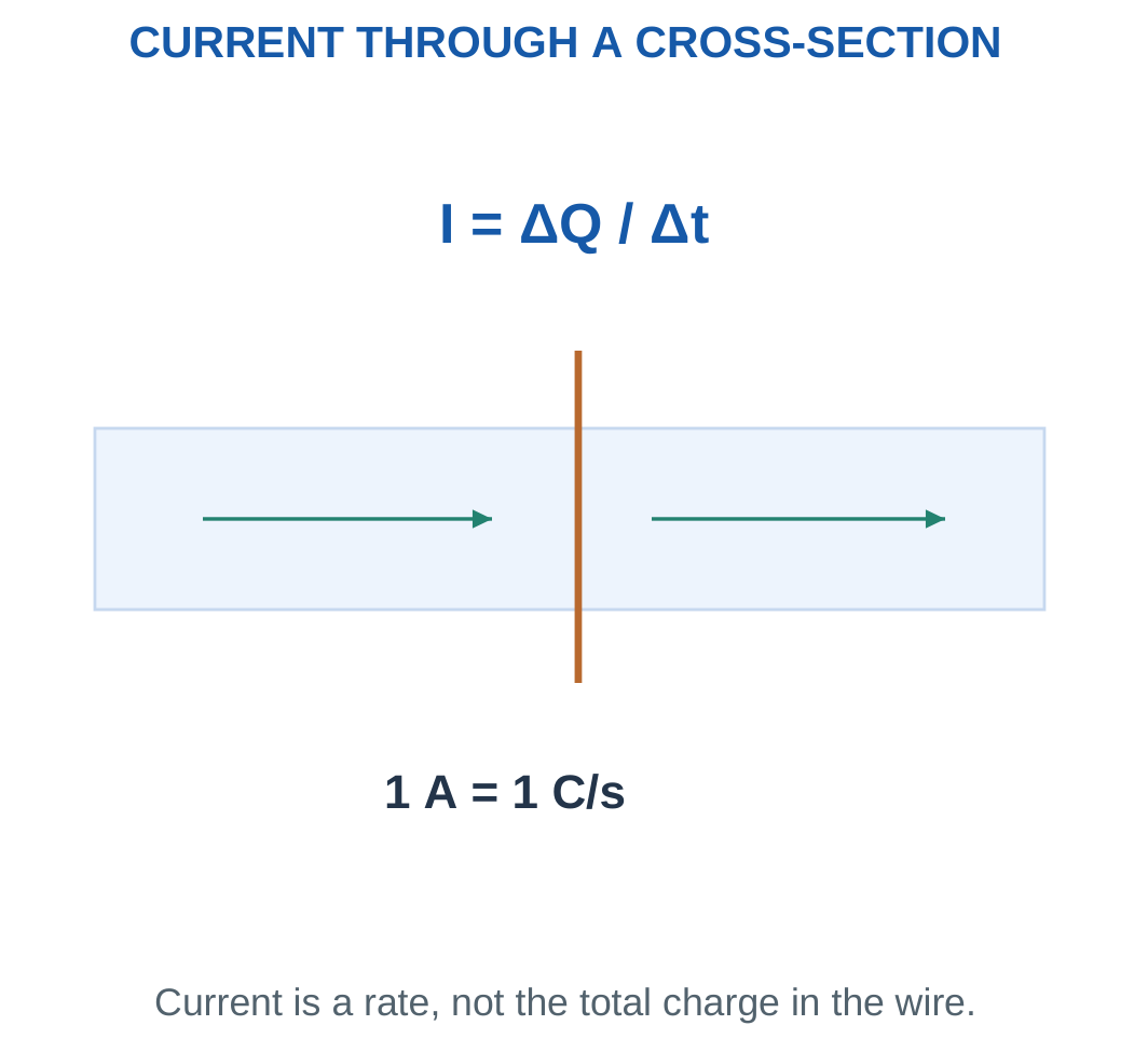
One ampere means one coulomb per second. A current of 2 A therefore represents a charge-transfer rate of 2 C each second at the selected cross-section.
Conventional current follows the direction positive charge would move. In an ordinary metallic conductor, electrons drift in the opposite direction. Circuit calculations use conventional current.
A current arrow is a reference. If an arrow is drawn from A to B and the solved current is −2 A, the actual conventional current is 2 A from B to A.
Changing an arrow after solving requires changing the sign of its variable. Silently reversing the arrow while retaining the same signed variable creates an inconsistent solution.
Time Conversion
Use seconds with amperes to obtain coulombs. A current of 100 mA for one minute transfers:
Q = 0.1 × 60 = 6 C.
It does not transfer 0.1 C or 100 C. The time conversion must be performed before interpreting the result.
Worked Problem 1.4: Charge Transferred at Constant Current
Problem: A constant 250 mA flows for 120 s. Find charge in coulombs and ampere-hours.
Step 1: Convert current.
I = 250 mA = 0.25 A.
Step 2: Calculate charge in coulombs.
Q = It = 0.25 × 120.
Q = 30 C.
Step 3: Calculate ampere-hours.
Charge = 0.25 × 120/3600.
Charge = 0.00833333 Ah.
Worked Problem 1.5: Charge at a Smaller Current
Problem: A constant 20 mA flows for 300 s. Find transferred charge in coulombs and ampere-hours.
I = 20 mA = 0.02 A.
Q = 0.02 × 300.
Q = 6 C.
Charge in Ah = 0.02 × 300/3600.
Charge = 0.00166667 Ah.
Worked Problem 1.6: Charge at a Larger Current
Problem: A constant 2000 mA flows for 30 s. Find transferred charge.
I = 2000 mA = 2 A.
Q = 2 × 30.
Q = 60 C.
Charge in Ah = 2 × 30/3600.
Charge ≈ 0.0167 Ah.
Worked Problem 1.7: Average Current over Two Intervals
Problem: Current is 2 A for 3 s and 0.5 A for the next 7 s in the same direction. Find total charge and average current.
Step 1: Calculate charge for each interval.
Q1 = 2 × 3 = 6 C.
Q2 = 0.5 × 7 = 3.5 C.
Step 2: Add charge and time.
Qtotal = 6 + 3.5 = 9.5 C.
ttotal = 3 + 7 = 10 s.
Step 3: Calculate average current.
Iavg = 9.5/10.
Iavg = 0.95 A.
The arithmetic average of the two current values would be incorrect because the intervals are unequal. Average current is total transferred charge divided by total elapsed time.
4. Voltage, Potential Difference and Energy per Charge
Voltage between two points expresses electrical potential difference.
Define:
VAB = VA − VB
A voltage of one volt corresponds to one joule of energy transfer per coulomb.
For a constant potential difference, the magnitude of energy transferred is:
W = VQ
The sign of an energy change requires attention to charge sign, motion direction and the chosen energy convention. When a question asks only for magnitude, use the magnitude of the voltage difference and the stated charge magnitude.

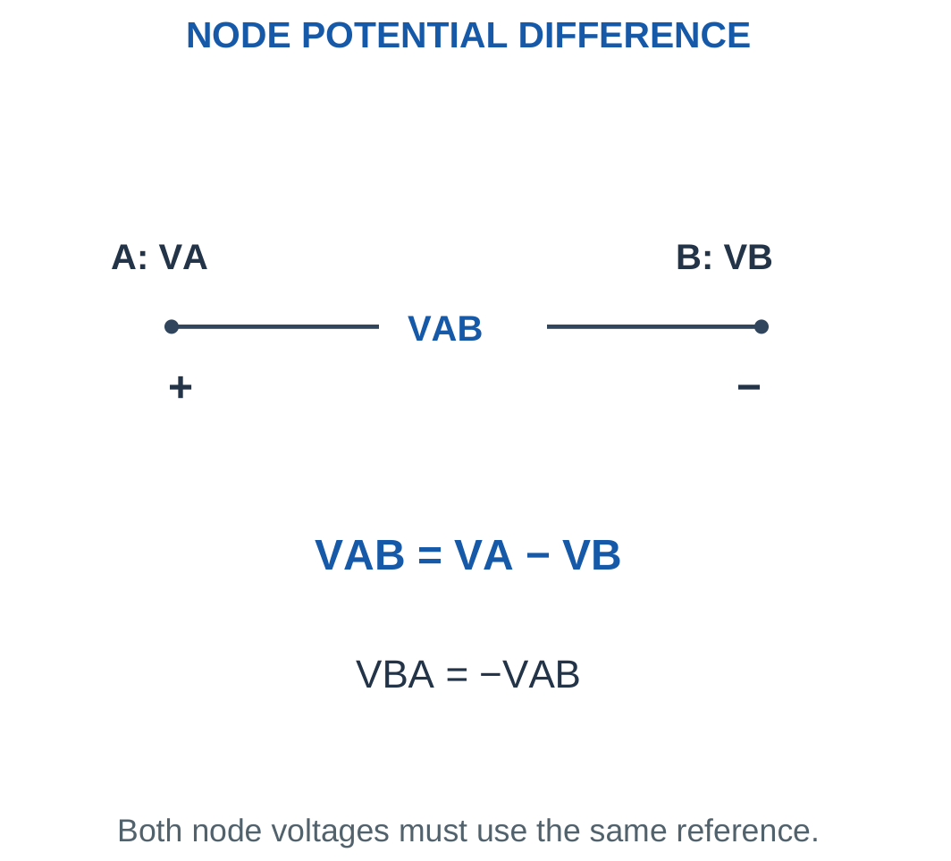
The reference node is assigned zero volts by choice. It does not have to be an earth electrode. If VA = 7 V and VB = 2 V relative to a common reference, then VAB = 5 V.
Choosing another reference shifts both node potentials by the same amount but does not change their difference. Circuit behaviour depends on potential differences rather than the arbitrary numerical value assigned to the reference node.
A component’s voltage polarity is independent of its chosen current reference until a sign convention is stated. In a positive resistor, actual conventional current enters the higher-potential terminal.
For a source, current may enter or leave the positive terminal. This distinction determines whether the source absorbs or delivers power.
Common Mistake
Voltage is measured across two points. Current is measured through a branch. Saying that voltage flows through a resistor mixes two different electrical quantities.
Worked Problem 1.8: Node Difference and Reversed Polarity
Problem: VA = 12 V and VB = 5 V relative to a common reference. Find VAB, VBA and the magnitude of energy associated with 2 C crossing this potential difference.
VAB = VA − VB.
VAB = 12 − 5.
VAB = 7 V.
VBA = −VAB.
VBA = −7 V.
Energy magnitude = |VAB|Q = 7 × 2.
Energy magnitude = 14 J.
Worked Problem 1.9: A Negative Node Potential
Problem: VA = 3 V and VB = −2 V. Find VAB, VBA and energy magnitude for 0.5 C.
VAB = 3 − (−2).
VAB = 5 V.
VBA = −5 V.
Energy magnitude = 5 × 0.5.
Energy magnitude = 2.5 J.
Subtracting a negative node potential increases the difference. The reference node does not prevent another node from having a negative potential.
Worked Problem 1.10: Negative Voltage Difference
Problem: VA = −4 V and VB = 1 V. Find VAB, VBA and energy magnitude for 3 C.
VAB = −4 − 1.
VAB = −5 V.
VBA = 5 V.
Energy magnitude = 5 × 3.
Energy magnitude = 15 J.
The negative VAB means A is 5 V below B. It does not mean the voltage difference lacks physical meaning.
5. EMF and Practical Source Terminal Voltage
Electromotive force, or EMF, is energy supplied by a source per unit charge.
E = Energy supplied / Charge
Its unit is the volt. Despite the historical word force, EMF is not a mechanical force measured in newtons.
An ideal voltage source maintains its specified terminal voltage regardless of current in the mathematical model. A practical source may be represented by an ideal EMF E in series with internal resistance r.

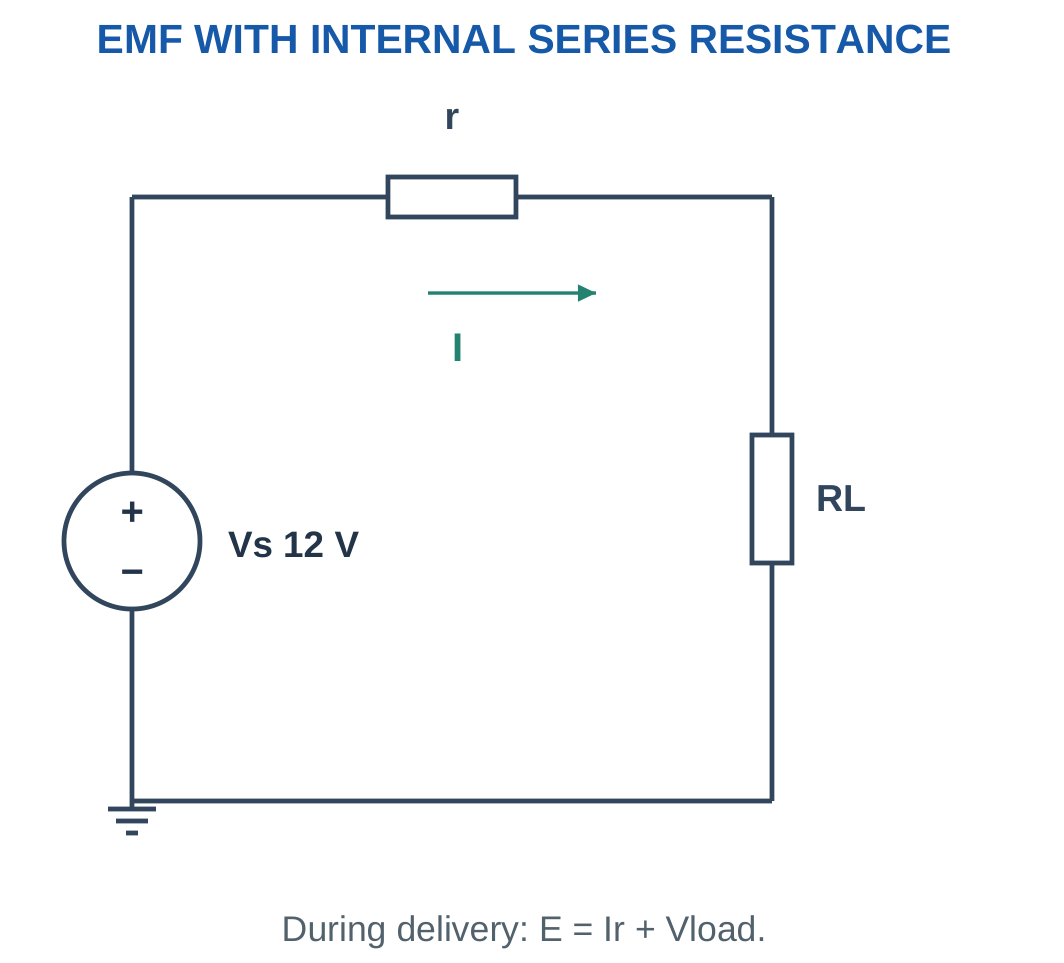
For the stated series-resistance model delivering current I:
Vterminal = E − Ir
With external load RL:
I = E/(r + RL)
Vterminal = IRL
Internal resistor heating is:
Pinternal = I²r
At open circuit, I = 0 and the model gives Vterminal = E. During delivery through nonzero internal resistance, terminal voltage is below EMF.
If current enters the source’s positive terminal, the source can absorb power. The terminal relationship must then be interpreted using the signed current reference. An unsigned charging current should not be inserted blindly into a discharge formula.
Idealisation
An ideal source’s ability to maintain voltage is a mathematical property of the model. It does not establish that a real battery can provide unlimited current.
Worked Problem 1.11: EMF versus Terminal Voltage
Problem: A source has EMF 12 V and internal resistance 1 Ω. It supplies a 5 Ω load. Find current, terminal voltage and internal power.
I = E/(r + RL).
I = 12/(1 + 5).
I = 2 A.
Vterminal = E − Ir.
Vterminal = 12 − 2 × 1.
Vterminal = 10 V.
Pinternal = I²r = 2² × 1.
Pinternal = 4 W.
Load power is 2² × 5 = 20 W. The ideal EMF supplies 12 × 2 = 24 W, equal to load power plus internal heating.
Worked Problem 1.12: A 9 V Source Model
Problem: E = 9 V, r = 0.5 Ω and RL = 4 Ω. Find current, terminal voltage and internal loss.
I = 9/(0.5 + 4).
I = 2 A.
Vterminal = 9 − 2 × 0.5.
Vterminal = 8 V.
Pinternal = 2² × 0.5.
Pinternal = 2 W.
Worked Problem 1.13: A 6 V Source Model
Problem: E = 6 V, r = 0.2 Ω and RL = 2.8 Ω. Find current, terminal voltage and internal power.
I = 6/(0.2 + 2.8).
I = 2 A.
Vterminal = 6 − 2 × 0.2.
Vterminal = 5.6 V.
Pinternal = 2² × 0.2.
Pinternal = 0.8 W.
The external load receives 5.6 V rather than the complete 6 V EMF because the internal resistance develops a 0.4 V drop.
6. Resistance, Resistivity and Conductor Geometry
Resistance relates the voltage across an element to its current under stated operating conditions.
For a uniform conductor:
R = ρL/A
where:
- R is resistance in ohms.
- ρ is resistivity in Ω·m.
- L is conductor length in metres.
- A is conducting cross-sectional area in square metres.

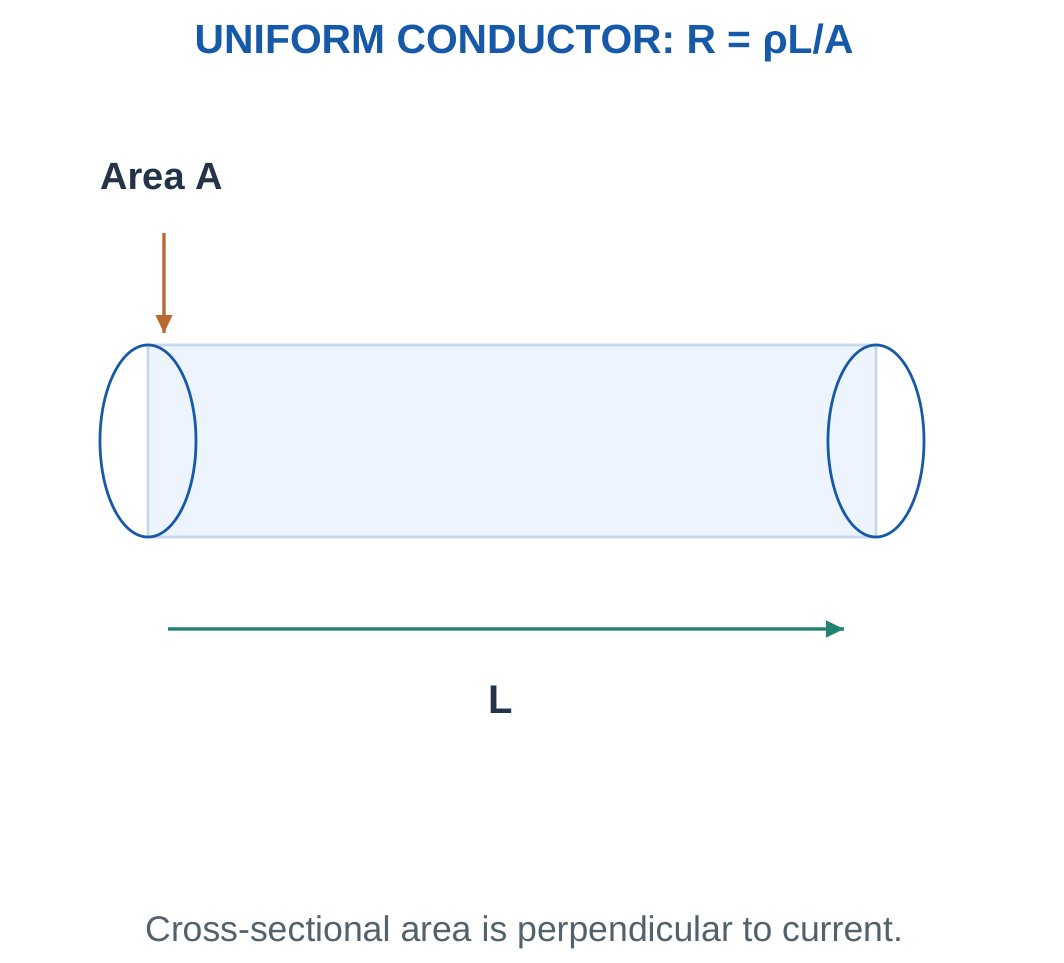
Resistivity is a material property under specified conditions such as temperature. Resistance depends on both the material property and geometry. Their units and meanings are different.
Doubling the length doubles resistance when area and resistivity remain unchanged. Doubling area halves resistance when the other quantities remain unchanged.
If length and area both change, include both factors. For example, doubling length and halving area multiplies resistance by four.
The conducting area is the metal cross-section, not the overall diameter including insulation. When a cable contains a separate return conductor, the specified current path may require including both outgoing and return lengths.
For a positive linear resistor, resistance remains constant within the assumed operating range. Real components have tolerances, temperature dependence and maximum power ratings.
Unit Trap
One square millimetre is:
1 mm² = 10⁻⁶ m²
It is not 10⁻³ m². Area conversion requires squaring the length conversion.
Worked Problem 1.14: Resistance from Geometry
Problem: A conductor has resistivity 1.7 × 10⁻⁸ Ω·m, length 20 m and cross-section 1 mm². Find resistance.
Step 1: Convert area.
A = 1 × 10⁻⁶ m².
Step 2: Apply the conductor formula.
R = ρL/A.
R = (1.7 × 10⁻⁸ × 20)/(1 × 10⁻⁶).
R = 0.34 Ω.
Worked Problem 1.15: A Longer, Thicker Conductor
Problem: Resistivity is 1.7 × 10⁻⁸ Ω·m, length is 50 m and area is 2.5 mm². Find resistance.
A = 2.5 × 10⁻⁶ m².
R = (1.7 × 10⁻⁸ × 50)/(2.5 × 10⁻⁶).
R = 0.34 Ω.
This conductor has the same resistance as the previous example because the increase in length is matched by the increase in conducting area.
Conductor Cross-Section

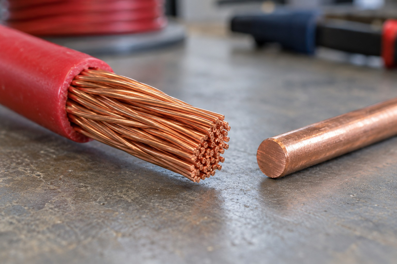
Conductor resistance depends on material, length and cross-sectional area in the stated model. Insulation thickness is not conducting area. Geometry and temperature must be matched when comparing two conductors.
7. Ohm’s Law and the Voltage–Current Characteristic
For an ohmic resistor under constant physical conditions:
V = IR
Equivalent forms are:
I = V/R
R = V/I
The measured voltage and current must refer to the same resistor and use a consistent polarity convention.

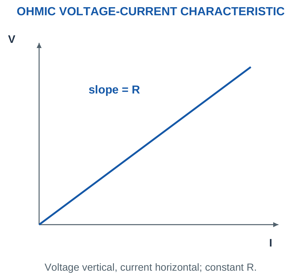
When voltage is on the vertical axis and current on the horizontal axis:
Slope = ΔV/ΔI = R
When current is vertical and voltage horizontal:
Slope = ΔI/ΔV = 1/R = G
The axes must therefore be identified before interpreting the slope.
For a nonlinear device, the ratio V/I at one operating point and the local slope need not be equal. Constant-resistance Ohm’s law is a particular linear model.
A resistor does not independently choose both its voltage and its current. The source and network determine their compatible values.
For example, a 10 Ω resistor across 5 V carries 0.5 A. Replacing it with 20 Ω at the same voltage reduces current to 0.25 A.
Model Boundary
Use the constant resistance stated in the problem. Do not introduce diode voltage drops, transistor operating regions or AC reactance into a resistive DC example unless the problem includes those elements.
Worked Problem 1.16: Resistor Current and Power
Problem: A 24 Ω resistor has 12 V across it. Find current and absorbed power.
I = 12/24.
I = 0.5 A = 500 mA.
P = V²/R = 12²/24.
P = 6 W.
Worked Problem 1.17: A Kilohm Resistor
Problem: A 1000 Ω resistor has 5 V across it.
I = 5/1000.
I = 0.005 A = 5 mA.
P = 5²/1000.
P = 0.025 W = 25 mW.
Worked Problem 1.18: A 120 Ω Resistor
Problem: A 120 Ω resistor has 24 V across it.
I = 24/120.
I = 0.2 A = 200 mA.
P = 24²/120.
P = 4.8 W.
Worked Problem 1.19: A 2.2 kΩ Resistor
Problem: A 2200 Ω resistor has 3.3 V across it.
I = 3.3/2200.
I = 0.0015 A = 1.5 mA.
P = 3.3²/2200.
P = 0.00495 W = 4.95 mW.
Worked Problem 1.20: Read a Graph Slope
Problem: A graph has voltage vertical and current horizontal. It passes through 2 V at 0.1 A and 6 V at 0.3 A. Find resistance and the reciprocal graph slope.
R = ΔV/ΔI.
R = (6 − 2)/(0.3 − 0.1).
R = 20 Ω.
For the current-versus-voltage graph:
G = 1/R = 1/20.
G = 0.05 S.
The numerical slope has a different unit when the axes are reversed. The resistance has not changed; only the plotted relationship has been reversed.
8. Conductance and Engineering Units
Conductance is the reciprocal of resistance:
G = 1/R
Its SI unit is the siemens, S.
Ohm’s law can be written:
I = GV
Conductance is useful for parallel networks because parallel branch conductances add directly.
| Prefix | Multiplier | Example |
|---|---|---|
| Mega, M | 10⁶ | 1 MΩ = 1,000,000 Ω |
| Kilo, k | 10³ | 1 kΩ = 1000 Ω |
| Milli, m | 10⁻³ | 1 mA = 0.001 A |
| Micro, µ | 10⁻⁶ | 1 µA = 0.000001 A |
A convenient circuit combination is volts divided by kilohms giving milliamperes:
V/kΩ = mA
Similarly:
mA × kΩ = V
Power requires its own unit check:
V × mA = mW
Using A² with Ω gives watts, while using mA² with kΩ gives milliwatts after consistent scaling.


Reciprocal Check
A resistance of 1 kΩ has conductance 1 mS.
It does not have conductance 1 kS. Taking a reciprocal changes the numerical scale as well as the unit.
Worked Problem 1.21: Resistance to Conductance
Problem: Find conductance of 500 Ω in S and mS, and current at 10 V.
G = 1/500.
G = 0.002 S = 2 mS.
I = GV = 0.002 × 10.
I = 0.02 A = 20 mA.
Worked Problem 1.22: A 2000 Ω Resistance
G = 1/2000.
G = 0.0005 S = 0.5 mS.
At 10 V:
I = 0.0005 × 10.
I = 0.005 A = 5 mA.
Worked Problem 1.23: A 1 MΩ Resistance
G = 1/1,000,000.
G = 1 × 10⁻⁶ S = 0.001 mS.
At 10 V:
I = 10 × 10⁻⁶ A.
I = 10 µA = 0.01 mA.
A large resistance corresponds to a small conductance. This reciprocal behaviour is a useful immediate check before completing a calculation.
9. Nodes, Branches, Loops, Opens and Shorts
A node consists of points joined by ideal conductor. These points share one potential.
A branch is a path between nodes containing an element or a defined series path. A loop is a closed path through the circuit. A mesh is a loop containing no other loop inside it in a planar circuit drawing.

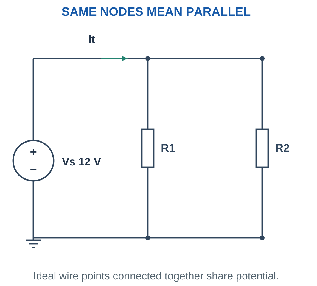
Two resistors are in series when the same current must pass through both without dividing at their common junction.
Two resistors are in parallel when both terminals share the same two nodes. Sharing only one node does not make them parallel.
A bridge-shaped network may not permit an immediate series or parallel reduction. The arrangement of symbols can hide the actual node relationships, so node labels should be established before combining components.
An ideal open branch enforces:
Iopen = 0
It can support a nonzero terminal voltage.
An ideal short circuit enforces:
Vshort = 0
It can carry a nonzero current determined by the surrounding network.
A resistor bypassed by an ideal wire has zero voltage across it. Therefore its current is zero for a positive finite resistance, while the wire may carry the complete path current.
Redraw Intelligently
Move ideal wires and stretch the drawing without changing connectivity. Label the nodes before deciding which components combine.
A redraw is useful only when it preserves every connection. Accidentally joining two distinct nodes produces a different circuit.
Worked Problem 1.24: Open Load with a Series Resistor
Problem: A 12 V source connects through 1 kΩ to open terminal a. Terminal b is the source negative reference. Find current, resistor drop and Vab.
The open output prevents a complete current path.
I = 0 A.
Resistor drop:
VR = IR = 0 × 1000.
VR = 0 V.
Terminal a remains at source positive potential:
Vab = 12 V.
An open branch can therefore have a nonzero voltage even though its current is zero.
Worked Problem 1.25: A Bypassed Resistor
Problem: A 10 Ω resistor is connected in parallel with an ideal wire between A and B. The surrounding circuit carries 2 A through the combined path. Find resistor voltage and current.
The wire forces:
VAB = 0 V.
The resistor shares those terminals:
Iresistor = 0/10.
Iresistor = 0 A.
The stated 2 A therefore passes through the ideal wire in this model.
10. Resistors Connected in Series
Series resistors carry the same branch current.
Applying KVL:
V = IR1 + IR2 + IR3 + …
Factoring out current:
V = I(R1 + R2 + R3 + …).
Therefore:
Req = R1 + R2 + R3 + …

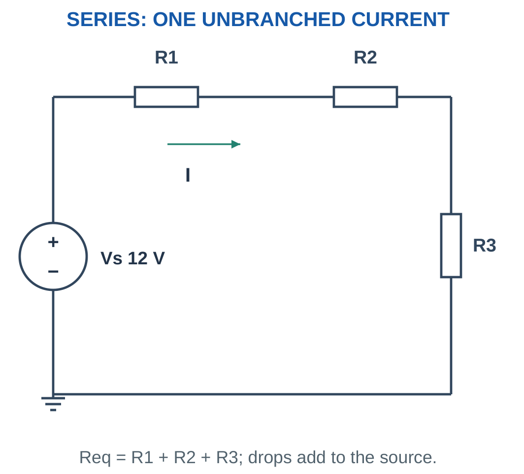
For a source V across the complete chain:
I = V/Req
Individual drops are:
Vi = IRi
The total positive series resistance is greater than any individual constituent.
For n identical resistors:
Req = nR
If one element becomes open, the ideal series-path current becomes zero. The resulting voltage distribution must be reconsidered; the previous operating drops cannot simply be retained.
Series resistors do not necessarily dissipate equal power. Since current is common:
Pi = I²Ri
The larger resistance dissipates more power at that common current.
Sanity Check
If a positive series equivalent is smaller than one of its components, either the topology or the arithmetic is wrong.
Worked Problem 1.26: Series Equivalent, Drops and Powers
Problem: A 12 V source drives 2 Ω, 4 Ω and 6 Ω in series.
Req = 2 + 4 + 6.
Req = 12 Ω.
I = 12/12.
I = 1 A.
Individual drops:
- V1 = 1 × 2 = 2 V.
- V2 = 1 × 4 = 4 V.
- V3 = 1 × 6 = 6 V.
Individual powers:
- P1 = 1² × 2 = 2 W.
- P2 = 1² × 4 = 4 W.
- P3 = 1² × 6 = 6 W.
The drops add to 12 V and the powers add to source power, 12 W.
Worked Problem 1.27: A 24 V Series Network
Problem: A 24 V source drives 3 Ω, 5 Ω and 4 Ω in series.
Req = 3 + 5 + 4.
Req = 12 Ω.
I = 24/12.
I = 2 A.
Drops in listed order are:
6 V, 10 V and 8 V.
Powers in listed order are:
12 W, 20 W and 16 W.
Total absorbed power is 48 W, equal to 24 × 2.
Resistors Connected in a Single Path

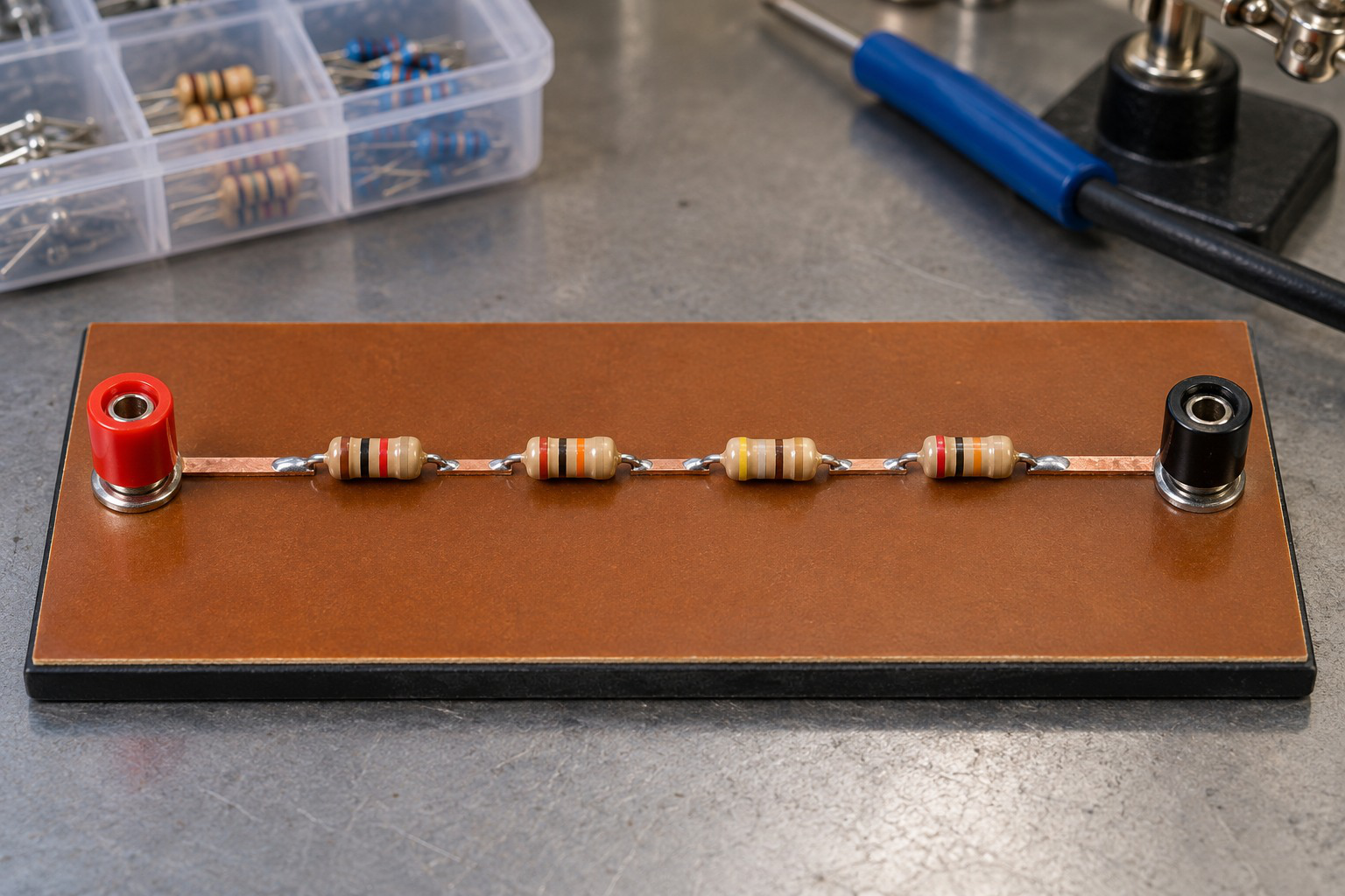
Series elements share branch current. Their individual drops and powers depend on their resistance values. Schematic connections rather than physical spacing define the series relationship.
Worked Problem 1.28: Series Resistors in Ohms
Problem: A 9 V source drives 150 Ω, 300 Ω and 450 Ω in series.
Req = 150 + 300 + 450.
Req = 900 Ω.
I = 9/900.
I = 0.01 A = 10 mA.
Drops are:
1.5 V, 3 V and 4.5 V.
Powers are:
0.015 W, 0.03 W and 0.045 W.
Their sum is 0.09 W, equal to source power 9 × 0.01.
11. Resistors Connected in Parallel
Parallel resistors share the same two terminal nodes. Therefore they have the same voltage.
For parallel branches:
I1 = V/R1.
I2 = V/R2.
I3 = V/R3.
KCL gives:
It = V/R1 + V/R2 + V/R3.
Therefore:
1/Req = 1/R1 + 1/R2 + 1/R3 + …
For two resistors:
Req = R1R2/(R1 + R2)

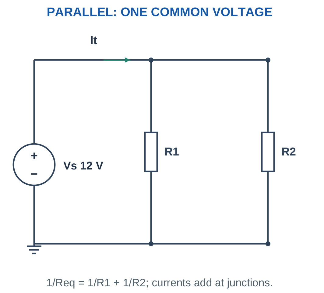
For positive finite parallel resistors, equivalent resistance is smaller than the smallest branch resistance.
For n equal branches:
Req = R/n
A lower-resistance branch draws more current at the common voltage. Adding another positive parallel branch increases total conductance and reduces equivalent resistance.
Under an ideal fixed-voltage source, existing branch voltages remain unchanged when another parallel branch is added. A practical source with internal resistance can behave differently because its terminal voltage depends on total current.
Two-Resistor Shortcut
The product-over-sum formula applies directly to two parallel resistors. For three or more resistors, use the reciprocal sum or combine a valid pair first.
Do not multiply all resistances and divide by their simple sum for a three-branch network. That expression is not the general parallel formula.
Worked Problem 1.29: Two Parallel Branches
Problem: Resistors 6 Ω and 12 Ω are connected across 12 V.
1/Req = 1/6 + 1/12.
Req = 4 Ω.
I1 = 12/6.
I1 = 2 A.
I2 = 12/12.
I2 = 1 A.
It = 2 + 1.
It = 3 A.
Source current from the equivalent is 12/4 = 3 A, confirming the result.
Worked Problem 1.30: Three Parallel Branches
Problem: Resistors 12 Ω, 24 Ω and 8 Ω are connected across 24 V.
1/Req = 1/12 + 1/24 + 1/8.
Req = 4 Ω.
Branch currents are:
- I1 = 24/12 = 2 A.
- I2 = 24/24 = 1 A.
- I3 = 24/8 = 3 A.
It = 6 A.
The 8 Ω branch draws the greatest current because it has the smallest resistance.
Worked Problem 1.31: Parallel Kilohm Resistors
Problem: Resistors 1000 Ω and 2000 Ω are across 5 V.
Req = (1000 × 2000)/(1000 + 2000).
Req = 666.6667 Ω.
I1 = 5/1000 = 5 mA.
I2 = 5/2000 = 2.5 mA.
It = 7.5 mA.
Parallel Load Branches

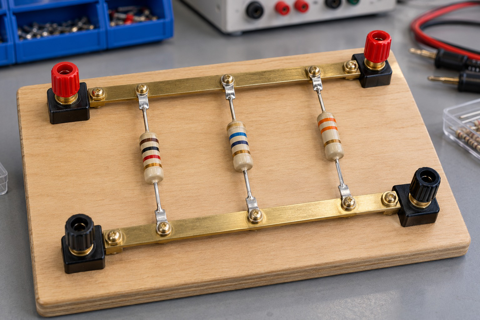
Parallel branches share one node-pair voltage while current divides. Branch currents add at the junction. A negative signed result reverses the chosen reference direction without invalidating charge conservation.
12. Series–Parallel Network Reduction
A mixed resistor network is reduced one valid combination at a time.
The basic procedure is:
- Identify the actual nodes.
- Find a genuine series chain or parallel group.
- Replace that group with its equivalent.
- Redraw the remaining circuit.
- Continue until the source sees one equivalent resistance.
- Calculate source current.
- Work backward to recover original branch voltages and currents.


For R1 in series with R2 parallel to R3:
Rp = R2R3/(R2 + R3)
Rt = R1 + Rp
It = Vs/Rt
Vparallel = ItRp
I2 = Vparallel/R2
I3 = Vparallel/R3
Do not use the complete source voltage across R2 or R3 when R1 develops a nonzero series drop.
Do not assign source current to every parallel branch. Source current divides at the junction, and the individual branch currents must add back to it.
Verification Habit
Check KCL at the current split and KVL around either complete source-to-return path. In a purely resistive ideal-source network, total resistor power must equal source power.
Worked Problem 1.32: Reduce and Recover Every Branch


Problem: A 12 V source drives 2 Ω in series with 6 Ω parallel to 3 Ω.
Rp = (6 × 3)/(6 + 3).
Rp = 2 Ω.
Rt = 2 + 2.
Rt = 4 Ω.
It = 12/4.
It = 3 A.
Vparallel = 3 × 2.
Vparallel = 6 V.
I2 = 6/6.
I2 = 1 A.
I3 = 6/3.
I3 = 2 A.
The branch currents add to 3 A. The series resistor drops 6 V, leaving 6 V across the parallel combination.
Worked Problem 1.33: A Scaled Mixed Network

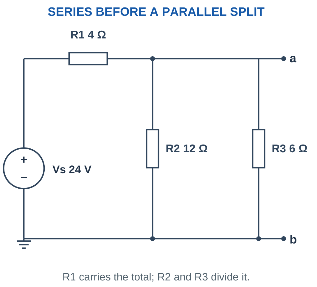
Problem: Vs = 24 V, R1 = 4 Ω, R2 = 12 Ω and R3 = 6 Ω.
Rp = (12 × 6)/(12 + 6).
Rp = 4 Ω.
Rt = 4 + 4.
Rt = 8 Ω.
It = 24/8.
It = 3 A.
Vparallel = 3 × 4.
Vparallel = 12 V.
I2 = 12/12 = 1 A.
I3 = 12/6 = 2 A.
The current split is 1 A and 2 A.
Worked Problem 1.34: Equal Parallel Branches

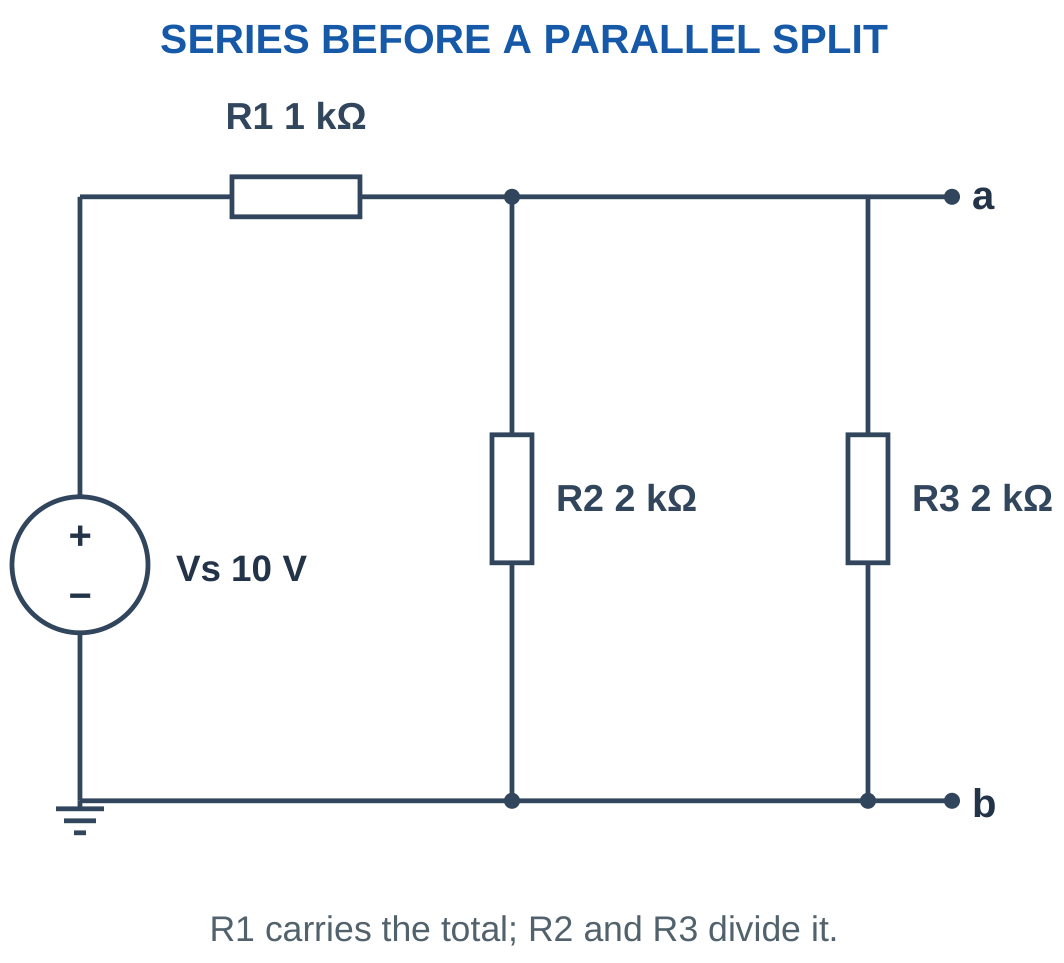
Problem: Vs = 10 V, R1 = 1000 Ω, R2 = 2000 Ω and R3 = 2000 Ω.
Rp = 2000/2.
Rp = 1000 Ω.
Rt = 1000 + 1000.
Rt = 2000 Ω.
It = 10/2000.
It = 5 mA.
Vparallel = 0.005 × 1000.
Vparallel = 5 V.
I2 = 5/2000 = 2.5 mA.
I3 = 5/2000 = 2.5 mA.
The equal branch currents add to 5 mA as required.
Worked Problem 1.35: Unequal Lower Branches


Problem: Vs = 18 V, R1 = 3 Ω, R2 = 12 Ω and R3 = 4 Ω.
Rp = (12 × 4)/(12 + 4).
Rp = 3 Ω.
Rt = 3 + 3.
Rt = 6 Ω.
It = 18/6.
It = 3 A.
Vparallel = 3 × 3.
Vparallel = 9 V.
I2 = 9/12.
I2 = 0.75 A.
I3 = 9/4.
I3 = 2.25 A.
The lower-resistance branch receives three times the current of the higher-resistance branch.
13. Voltage-Divider Rule
An unloaded voltage divider consists of series resistors across a source, with output measured across a selected resistor or series group.
For R1 and R2 across Vs:
I = Vs/(R1 + R2).
Voltage across R2 is:
Vout = IR2.
Therefore:
Vout = VsR2/(R1 + R2)
For a larger series chain:
Vi = VsRi/ΣR


The output fraction depends on the resistance ratio. Total divider current depends on total resistance.
Scaling both resistors by the same positive factor preserves unloaded output voltage. However, it changes divider current, resistor power and sensitivity to an external load.
For a desired fraction a = Vout/Vs:
R2/R1 = a/(1 − a)
This applies for 0 < a < 1 in the simple positive-resistance ground-referenced divider.
Do Not Memorise Blindly
Mark output terminals before selecting the numerator. Voltage across R1 uses R1 in the numerator, while voltage across R2 uses R2.
A passive unloaded divider cannot produce an output larger than the applied source magnitude under this simple arrangement.
Worked Problem 1.36: Unloaded Divider
Problem: Vs = 12 V, R1 = 2000 Ω and R2 = 1000 Ω. Find output across R2 and divider current.
I = 12/(2000 + 1000).
I = 4 mA.
Vout = 12 × 1000/3000.
Vout = 4 V.
The upper resistor develops the remaining 8 V.
Worked Problem 1.37: A 10 V Divider
Problem: Vs = 10 V, R1 = 3000 Ω and R2 = 2000 Ω.
I = 10/5000.
I = 2 mA.
Vout = 10 × 2000/5000.
Vout = 4 V.
Worked Problem 1.38: Equal Divider Resistors
Problem: Vs = 5 V and both resistors are 10 kΩ.
I = 5/20,000.
I = 0.25 mA.
Vout = 5 × 10,000/20,000.
Vout = 2.5 V.
Equal series resistances divide the applied voltage equally when the output is unloaded.
Worked Problem 1.39: A One-Quarter Output
Problem: Vs = 24 V, R1 = 15 kΩ and R2 = 5 kΩ.
I = 24/20,000.
I = 1.2 mA.
Vout = 24 × 5000/20,000.
Vout = 6 V.
The lower resistor is one quarter of total resistance, so its voltage is one quarter of the source.
14. Loaded Voltage Divider and Measurement Loading
A load RL connected from the divider tap to reference is in parallel with the lower resistor R2.
The lower equivalent becomes:
Rlower = R2 || RL
The loaded output is:
Vout = Vs(R2 || RL)/[R1 + (R2 || RL)]

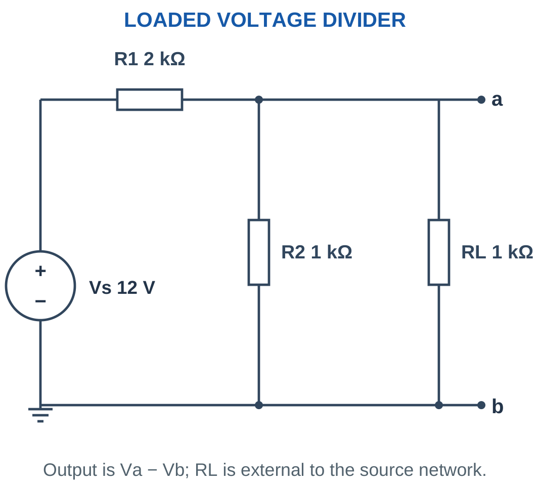
The original unloaded divider ratio is no longer exact after connecting a finite load.
A voltmeter with finite input resistance acts as a load. A high input resistance reduces loading error, but the error is not mathematically zero unless an ideal meter model is used.
For positive resistors under an ideal fixed source, a finite load across the lower leg reduces that leg’s equivalent resistance and lowers the tap voltage.
Choosing smaller divider resistors can reduce relative loading for a given external load, but increases divider current and power consumption.
Practical Interpretation
A divider is a voltage-scaling network. It does not automatically behave as a regulated power supply for a changing load.
The current through the upper resistor is the sum of lower-resistor current and external load current. Therefore load current must not be confused with total divider input current.
Worked Problem 1.40: Divider Loading Error

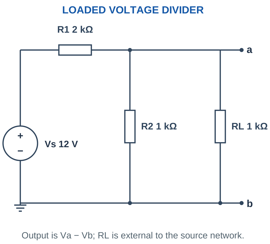
Problem: Vs = 12 V, R1 = 2000 Ω, R2 = 1000 Ω and RL = 1000 Ω.
Rlower = 1000 || 1000.
Rlower = 500 Ω.
Vloaded = 12 × 500/(2000 + 500).
Vloaded = 2.4 V.
IL = 2.4/1000.
IL = 2.4 mA.
Unloaded voltage:
V0 = 12 × 1000/3000.
V0 = 4 V.
Percentage reduction:
Reduction = (4 − 2.4)/4 × 100.
Reduction = 40%.
Worked Problem 1.41: Equal Divider and Load Resistances

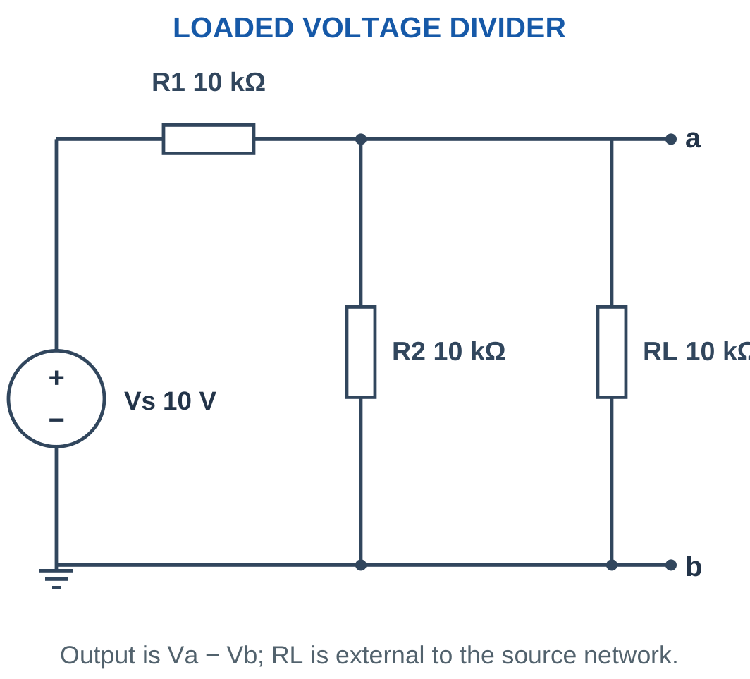
Problem: Vs = 10 V, R1 = 10 kΩ, R2 = 10 kΩ and RL = 10 kΩ.
Rlower = 10 kΩ || 10 kΩ.
Rlower = 5 kΩ.
Vloaded = 10 × 5/(10 + 5).
Vloaded ≈ 3.3333 V.
IL = 3.3333/10,000.
IL ≈ 0.3333 mA.
Unloaded voltage is 5 V.
Reduction = (5 − 3.3333)/5 × 100.
Reduction ≈ 33.3333%.
Worked Problem 1.42: A Relatively Light Load

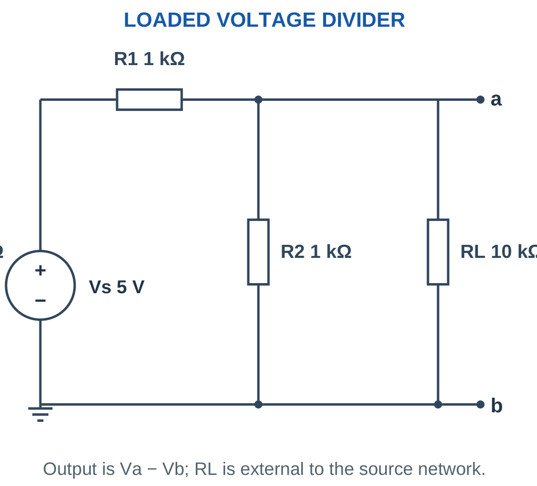
Problem: Vs = 5 V, R1 = 1000 Ω, R2 = 1000 Ω and RL = 10,000 Ω.
Rlower = (1000 × 10,000)/(1000 + 10,000).
Rlower ≈ 909.0909 Ω.
Vloaded = 5 × 909.0909/(1000 + 909.0909).
Vloaded ≈ 2.381 V.
IL = 2.381/10,000.
IL ≈ 0.2381 mA.
Unloaded voltage is 2.5 V.
Percentage reduction ≈ 4.7619%.
Worked Problem 1.43: A 24 V Loaded Divider


Problem: Vs = 24 V, R1 = 6000 Ω, R2 = 3000 Ω and RL = 6000 Ω.
Rlower = 3000 || 6000.
Rlower = 2000 Ω.
Vloaded = 24 × 2000/(6000 + 2000).
Vloaded = 6 V.
IL = 6/6000.
IL = 1 mA.
Unloaded output is:
V0 = 24 × 3000/9000 = 8 V.
Percentage reduction = 25%.
15. Current-Divider Rule
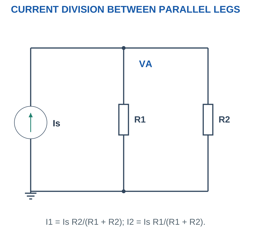
Parallel branches have the same voltage. Their currents are inversely proportional to their resistances.
For two branches:
I1 = ItR2/(R1 + R2)
I2 = ItR1/(R1 + R2)
The opposite resistor appears in each numerator.

For several parallel branches, conductance gives:
Ii = ItGi/ΣG
This follows because each branch current is GiV and total current is VΣG.
Confirm that the branches share both nodes before applying the rule. Components are not a current divider merely because they appear below the same line in a drawing.
If an ideal voltage source fixes the branch voltage, the currents can instead be found directly from V/R. Both approaches agree when applied to the same circuit.
Fast Checks
- Branch currents must add to total current.
- Equal parallel resistances receive equal currents.
- The smaller positive resistance receives the larger current.
- The common voltage calculated from either branch must agree.
Worked Problem 1.44: A 3 A Current Divider
Problem: Total current is 3 A through parallel 6 Ω and 3 Ω branches.
I1 through 6 Ω:
I1 = 3 × 3/(6 + 3).
I1 = 1 A.
I2 through 3 Ω:
I2 = 3 × 6/(6 + 3).
I2 = 2 A.
Common voltage:
V = 1 × 6 = 2 × 3.
V = 6 V.
Worked Problem 1.45: A 6 A Current Divider
Problem: It = 6 A, R1 = 4 Ω and R2 = 8 Ω.
I1 = 6 × 8/(4 + 8).
I1 = 4 A.
I2 = 6 × 4/(4 + 8).
I2 = 2 A.
V = 4 × 4 = 2 × 8.
V = 16 V.
Worked Problem 1.46: Current Division in Milliamperes
Problem: It = 12 mA, R1 = 1 kΩ and R2 = 2 kΩ.
I1 = 12 × 2/(1 + 2).
I1 = 8 mA.
I2 = 12 × 1/(1 + 2).
I2 = 4 mA.
Common voltage:
V = 8 mA × 1 kΩ.
V = 8 V.
Worked Problem 1.47: A 10 mA Divider
Problem: It = 10 mA, R1 = 3 kΩ and R2 = 6 kΩ.
I1 = 10 × 6/(3 + 6).
I1 ≈ 6.6667 mA.
I2 = 10 × 3/(3 + 6).
I2 ≈ 3.3333 mA.
V = 6.6667 mA × 3 kΩ.
V = 20 V.
The results satisfy the inverse-resistance relationship and add to the supplied current.
16. Power in DC Resistive Circuits
Electrical power is the rate at which energy is transferred.
Under the passive sign convention:
p = vi
when current enters the labelled positive-voltage terminal.
For a positive resistor:
P = VI = I²R = V²/R
Absorbed resistor power is nonnegative.

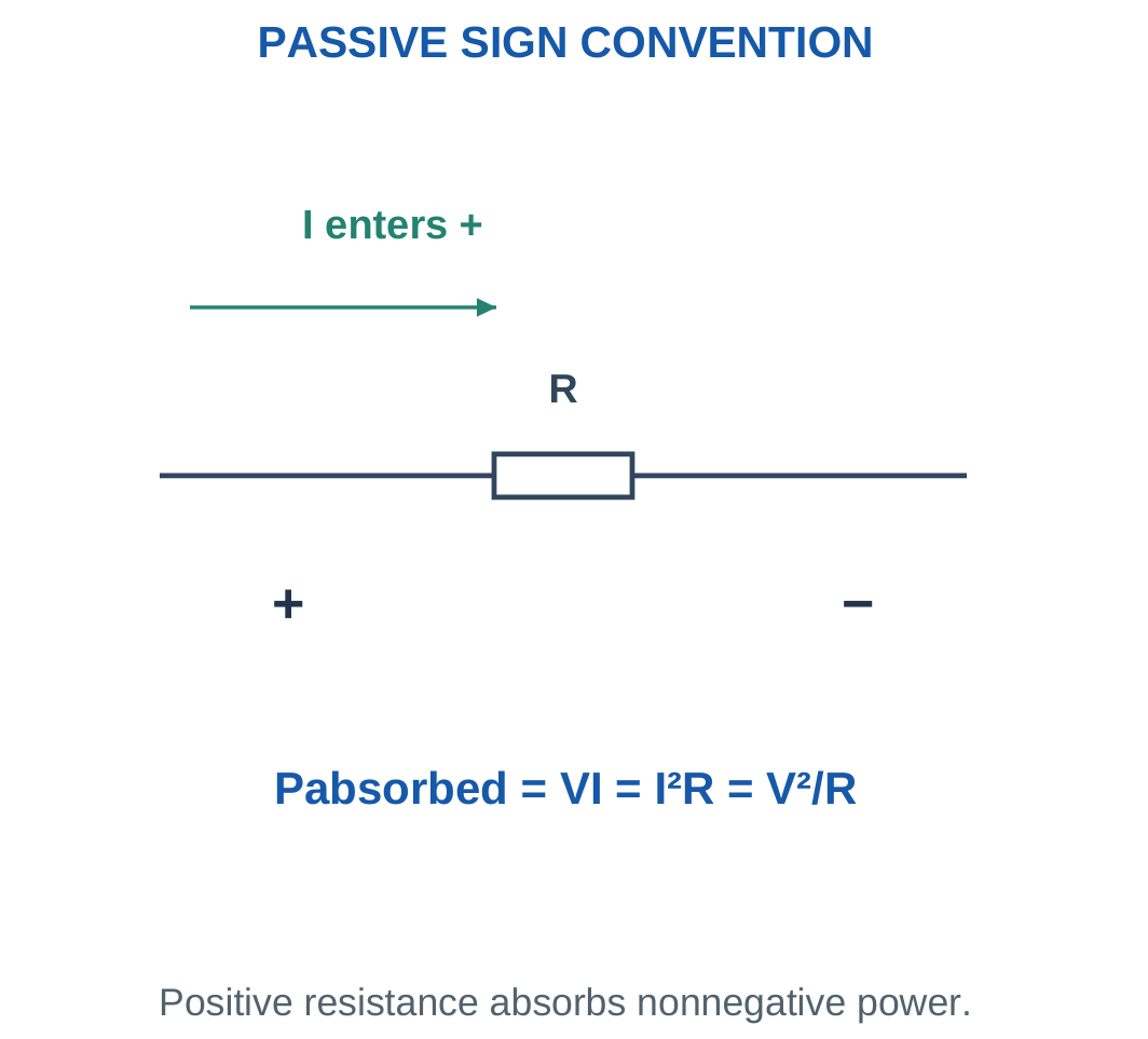
Use I²R when resistor current is known. Use V²/R when the resistor voltage is known.
A fixed-voltage comparison and a fixed-current comparison produce different trends:
- At fixed voltage, increasing R reduces power because P = V²/R.
- At fixed current, increasing R increases power because P = I²R.
These statements are consistent because the controlled quantity differs.
A resistor may have the required resistance value while being inadequately rated for calculated dissipation. Compare operating power with the supplied allowable rating under its stated conditions.
Unit Check
12 V × 20 mA = 240 mW = 0.24 W.
Writing 240 W would introduce a thousand-fold error.
Worked Problem 1.48: Rating Assessment
Problem: A 120 Ω resistor has 12 V across it. Its stated allowable dissipation is 0.5 W.
I = 12/120.
I = 0.1 A.
P = 12²/120.
P = 1.2 W.
Since 1.2 W exceeds 0.5 W, the stated nominal condition fails the rating comparison.
Worked Problem 1.49: A Lower Dissipation
Problem: A 100 Ω resistor has 5 V across it and a stated allowable dissipation of 0.5 W.
I = 5/100.
I = 0.05 A.
P = 5²/100.
P = 0.25 W.
The calculated dissipation is below the stated 0.5 W limit under the assumed conditions.
Worked Problem 1.50: A 24 V Load Resistor
Problem: A 240 Ω resistor has 24 V across it. Its allowable dissipation is stated as 3 W.
I = 24/240.
I = 0.1 A.
P = 24²/240.
P = 2.4 W.
The nominal comparison passes because 2.4 W is below 3 W. The assessment uses the specified operating and rating assumptions.
Resistive Load and Power Dissipation


A resistive load converts electrical energy into heat. Matching current and voltage are required for power calculation. Component size or the presence of a heat sink alone does not establish an acceptable temperature.
17. Source Power, Absorption and Power Balance
A source may supply or absorb energy depending on current direction relative to its voltage polarity.
Under the passive sign convention:
- Positive p = vi means absorption.
- Negative p = vi means delivery.
The word source identifies a circuit model. It does not mean that its power must always be negative.

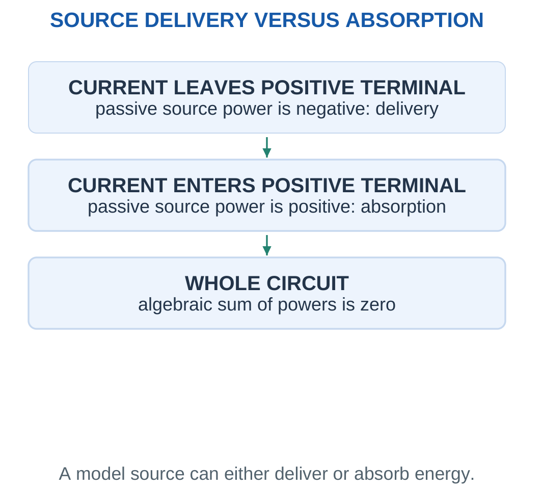
For a complete ideal resistive DC network:
Σp = 0
Equivalently:
Total delivered power = Total absorbed power
Include every source and resistor within the chosen circuit boundary.
When two voltage sources oppose through a resistor, the larger source can deliver energy partly to the resistor and partly to the other source model.
This is a mathematical statement about the supplied ideal models. It does not define a charging method for an arbitrary real battery.
Final Sign Check
Do not force every source power to be negative. Determine its sign from the solved current and marked voltage polarity.
A source whose current is zero has zero power even if its voltage is nonzero.
Worked Problem 1.51: One Source Delivers and Another Absorbs
Problem: Sources E1 = 12 V and E2 = 6 V have negative terminals joined. A 3 Ω resistor connects their positive terminals. Define current from E1 positive toward E2 positive.
I = (12 − 6)/3.
I = 2 A.
Current leaves E1 positive, so:
pE1 = −12 × 2.
pE1 = −24 W.
Current enters E2 positive, so:
pE2 = 6 × 2.
pE2 = 12 W.
Resistor power:
pR = 2² × 3.
pR = 12 W.
Power balance:
−24 + 12 + 12 = 0.
Worked Problem 1.52: A Second Opposing-Source Circuit
Problem: E1 = 10 V, E2 = 4 V and R = 2 Ω with the same references.
I = (10 − 4)/2.
I = 3 A.
pE1 = −10 × 3.
pE1 = −30 W.
pE2 = 4 × 3.
pE2 = 12 W.
pR = 3² × 2.
pR = 18 W.
Power balance:
−30 + 12 + 18 = 0.
Isolated Low-Voltage Bench Supply

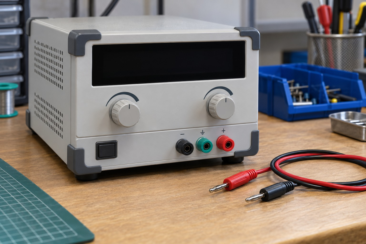
A supply provides circuit energy while the selected model defines its terminal voltage and internal behaviour. Current limiting and load conditions affect a real output.
A displayed setting should not be confused with a guaranteed voltage at every point in a loaded circuit. Lead resistance and internal source behaviour may matter when included in the model.
18. Energy, Watt-Hours and Running Cost
Power is an energy-transfer rate. Energy accumulates over time.
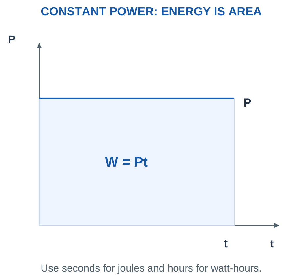
For constant power:
W = Pt
With P in watts and t in seconds, W is in joules.
With P in watts and t in hours, energy is in watt-hours.
1 Wh = 3600 J
1 kWh = 3.6 × 10⁶ J

For a supplied tariff calculation:
Cost = Energy in kWh × Rate per kWh
Add other charges only when the question specifies them.
The numerical tariffs below are hypothetical supplied values. They are used to demonstrate the calculation rather than represent a current electricity price.
For several loads or operating states:
Wtotal = ΣPiti
Charge capacity in Ah is not energy by itself. A voltage model is required to convert charge transfer into electrical energy.
Numerical Habit
Convert minutes to hours for Wh or to seconds for J. Carry the units through the multiplication.
Do not multiply a value in watts by minutes and then label the answer Wh without conversion.
Worked Problem 1.53: Energy and Hypothetical Cost
Problem: A 100 W load runs for 5 h. The supplied tariff is 8 currency units/kWh.
Energy = 100 × 5.
Energy = 500 Wh = 0.5 kWh.
In joules:
W = 500 × 3600.
W = 1,800,000 J.
Cost = 0.5 × 8.
Cost = 4 currency units.
Worked Problem 1.54: A 60 W Load
Problem: A 60 W load runs for 8 h. The hypothetical tariff is 7 currency units/kWh.
Energy = 60 × 8.
Energy = 480 Wh = 0.48 kWh.
W = 480 × 3600.
W = 1,728,000 J.
Cost = 0.48 × 7.
Cost = 3.36 currency units.
Worked Problem 1.55: A Higher-Power Load for a Shorter Time
Problem: A 1500 W load runs for 0.5 h. The supplied tariff is 6.5 currency units/kWh.
Energy = 1500 × 0.5.
Energy = 750 Wh = 0.75 kWh.
W = 750 × 3600.
W = 2,700,000 J.
Cost = 0.75 × 6.5.
Cost = 4.875 currency units.
Worked Problem 1.56: Two Operating States
Problem: A device draws 20 W for 2 h and 2 W for another 10 h. Find total energy and average power over those 12 h.
W1 = 20 × 2 = 40 Wh.
W2 = 2 × 10 = 20 Wh.
Wtotal = 60 Wh.
Pavg = Wtotal/ttotal.
Pavg = 60/12.
Pavg = 5 W.
The average is weighted by operating duration. It is not the arithmetic mean of 20 W and 2 W because those states last for different times.
19. Internal Resistance and Load Regulation
For a source with EMF E and series internal resistance r supplying RL:
I = E/(r + RL)
Terminal voltage is:
Vterminal = ERL/(r + RL)
Reducing RL increases current. The larger internal drop Ir then lowers terminal voltage in this model.

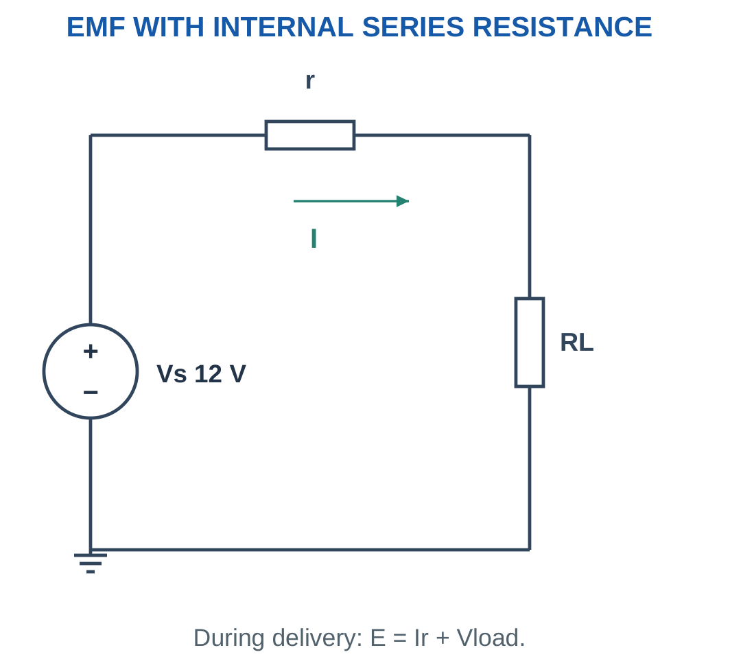
The internal resistance can represent a simplified source resistance or wiring resistance. It is separate from external load resistance.
If open-circuit EMF E and loaded terminal voltage V at current I are known:
r = (E − V)/I
This form uses the delivering-current convention.
At a mathematical external short with nonzero r, current is E/r and external terminal voltage is zero. Real sources may include additional protection and current-limit behaviour beyond this simple linear model.
Useful Comparison
An ideal source and a practical source can predict different effects when an additional parallel load is attached.
An ideal voltage source maintains branch voltage. A practical source may develop a greater internal drop because total current increases.
Worked Problem 1.57: Infer Internal Resistance
Problem: Open-circuit EMF is 12 V. At a delivered current of 2 A, terminal voltage is 11 V.
r = (12 − 11)/2.
r = 0.5 Ω.
Connected load resistance:
RL = 11/2.
RL = 5.5 Ω.
Internal drop is 1 V, consistent with 2 × 0.5.
Worked Problem 1.58: A 9 V Source
Problem: E = 9 V, terminal voltage is 8.4 V and current is 0.6 A.
r = (9 − 8.4)/0.6.
r = 1 Ω.
RL = 8.4/0.6.
RL = 14 Ω.
Worked Problem 1.59: A 6 V Source
Problem: E = 6 V, terminal voltage is 5.4 V and current is 1.5 A.
r = (6 − 5.4)/1.5.
r = 0.4 Ω.
RL = 5.4/1.5.
RL = 3.6 Ω.
The source model can now be used for another load only while its assumed linear behaviour remains applicable.
20. Kirchhoff’s Current Law
Kirchhoff’s Current Law states that the algebraic sum of currents at a node is zero in the steady lumped-circuit model.
ΣI = 0
An equivalent statement is:
Total current entering = Total current leaving
The law follows from conservation of charge when no net charge accumulates at the node.

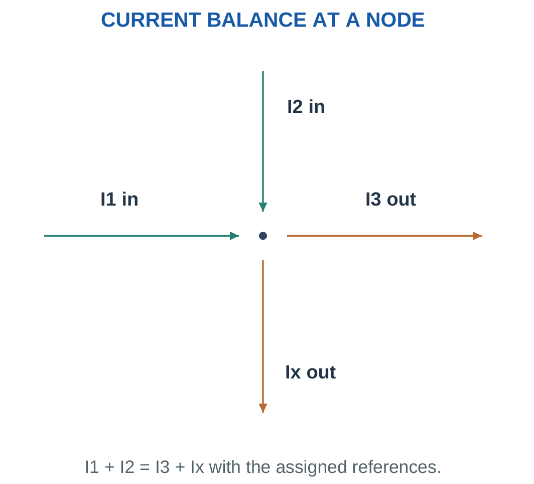
Choose one consistent convention:
- All currents leaving positive.
- All currents entering positive.
- Entering currents on one side and leaving currents on the other.
The conventions are equivalent when signs are handled consistently.
If 5 A and 2 A enter while 3 A and Ix leave:
5 + 2 = 3 + Ix.
Therefore Ix = 4 A.
A node can extend along an ideal wire containing several drawn junction dots. Those dots do not create separate node voltages when joined directly by ideal conductor.
KCL can also be applied to a larger closed boundary if every current crossing the boundary is included.
Avoid This Error
Current is not used up by a resistor. Current may split at a junction, but its algebraic balance remains zero.
A negative solved current should remain signed in the node equation and then be described in words using its actual direction.
Worked Problem 1.60: Positive Unknown Leaving Current
Problem: Currents 5 A and 2 A enter. A known 3 A leaves. Ix is referenced leaving.
7 = 3 + Ix.
Ix = 4 A leaving.
The positive result confirms the assigned leaving direction.
Worked Problem 1.61: KCL in Smaller Currents
Problem: Currents 0.02 A and 0.03 A enter. A known 0.01 A leaves. Ix is referenced leaving.
0.02 + 0.03 = 0.01 + Ix.
Ix = 0.04 A = 40 mA leaving.
All currents must use a consistent unit scale when substituted into the equation.
Worked Problem 1.62: Negative Unknown Current
Problem: Currents 1 A and 2 A enter. A known 5 A leaves. Ix is assumed leaving.
1 + 2 = 5 + Ix.
Ix = −2 A.
Actual current is:
2 A entering the node.
The negative result supplies the direction needed to satisfy charge conservation.
Worked Problem 1.63: A Negative Milliampere Result
Problem: Currents 6 mA and 4 mA enter. A known 12 mA leaves. Ix is referenced leaving.
6 + 4 = 12 + Ix.
Ix = −2 mA.
The physical current is 2 mA entering. Replacing the signed answer by positive 2 mA without reversing the interpreted direction would be incorrect.
21. Kirchhoff’s Voltage Law
Kirchhoff’s Voltage Law states that the algebraic sum of voltage changes around a closed path is zero for the lumped DC model.
ΣV = 0
A complete traversal returns to the initial potential. The law expresses consistent potential differences and energy transfer around the path.

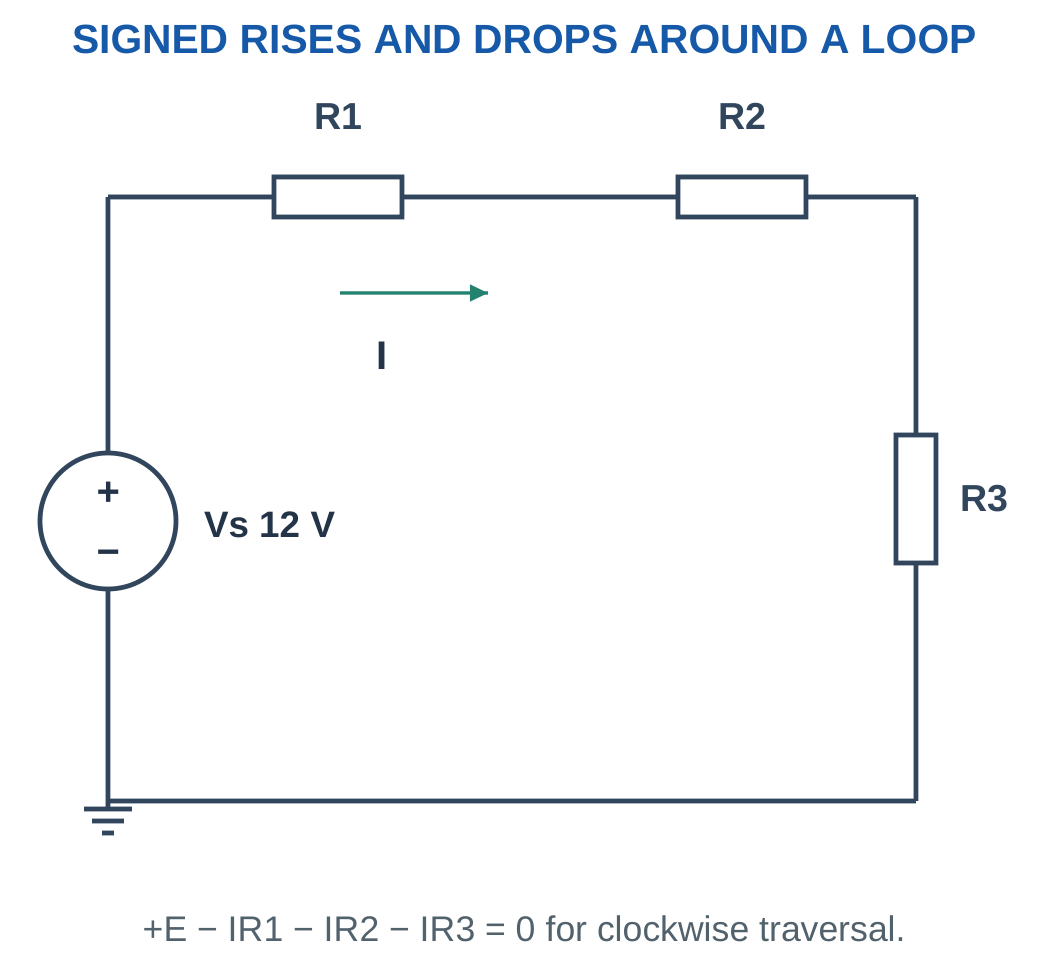
For resistor traversal:
- With its referenced current, use −IR as the potential change.
- Against its referenced current, use +IR.
For an ideal voltage source:
- From − to +, use +E.
- From + to −, use −E.
The source sign follows its polarity and traversal direction. It does not follow whether the source is drawn on the left or the right.
Reversing loop traversal multiplies every term by −1. It does not change the physical solution.
Self-Check
Never reverse only one term when reversing loop direction. Every potential change must follow the same traversal.
The same KVL equation can be written as rises equal drops or as an algebraic sum equal to zero.
Worked Problem 1.64: Solve a Single Loop
Problem: A 12 V source drives series 2 Ω and 4 Ω resistors.
Traverse from source negative to positive and then through the resistors with current.
12 − 2I − 4I = 0.
12 − 6I = 0.
I = 2 A.
Drops:
V1 = 2 × 2 = 4 V.
V2 = 2 × 4 = 8 V.
4 + 8 = 12 V.
Adjustable Resistance
A potentiometer can provide an adjustable divider. Its wiper voltage depends on connection and loading.
The total end-to-end resistance and the separate wiper segments are different quantities. Apply a divider equation only after identifying which segment is upper, which is lower and whether the wiper is loaded.
Worked Problem 1.65: A Kilohm Loop
Problem: A 10 V source drives 1 kΩ and 4 kΩ in series.
KVL:
10 − 1000I − 4000I = 0.
I = 10/5000.
I = 2 mA.
Drops:
V1 = 2 V.
V2 = 8 V.
The sum is 10 V.
Worked Problem 1.66: A 9 V Loop
Problem: A 9 V source drives 300 Ω and 600 Ω.
9 − 300I − 600I = 0.
I = 9/900.
I = 10 mA.
Drops:
V1 = 0.01 × 300 = 3 V.
V2 = 0.01 × 600 = 6 V.
3 + 6 = 9 V.
22. Branch Currents and Reference Choices
A branch current is the physical current through a selected branch with an assigned direction.
It is not always identical to a mesh-current variable. In a branch shared by two meshes, the physical branch current is an algebraic combination of the mesh currents.
For a resistor between A and B with current referenced from A to B:
IAB = (VA − VB)/R
Reversing the reference gives:
IBA = −IAB

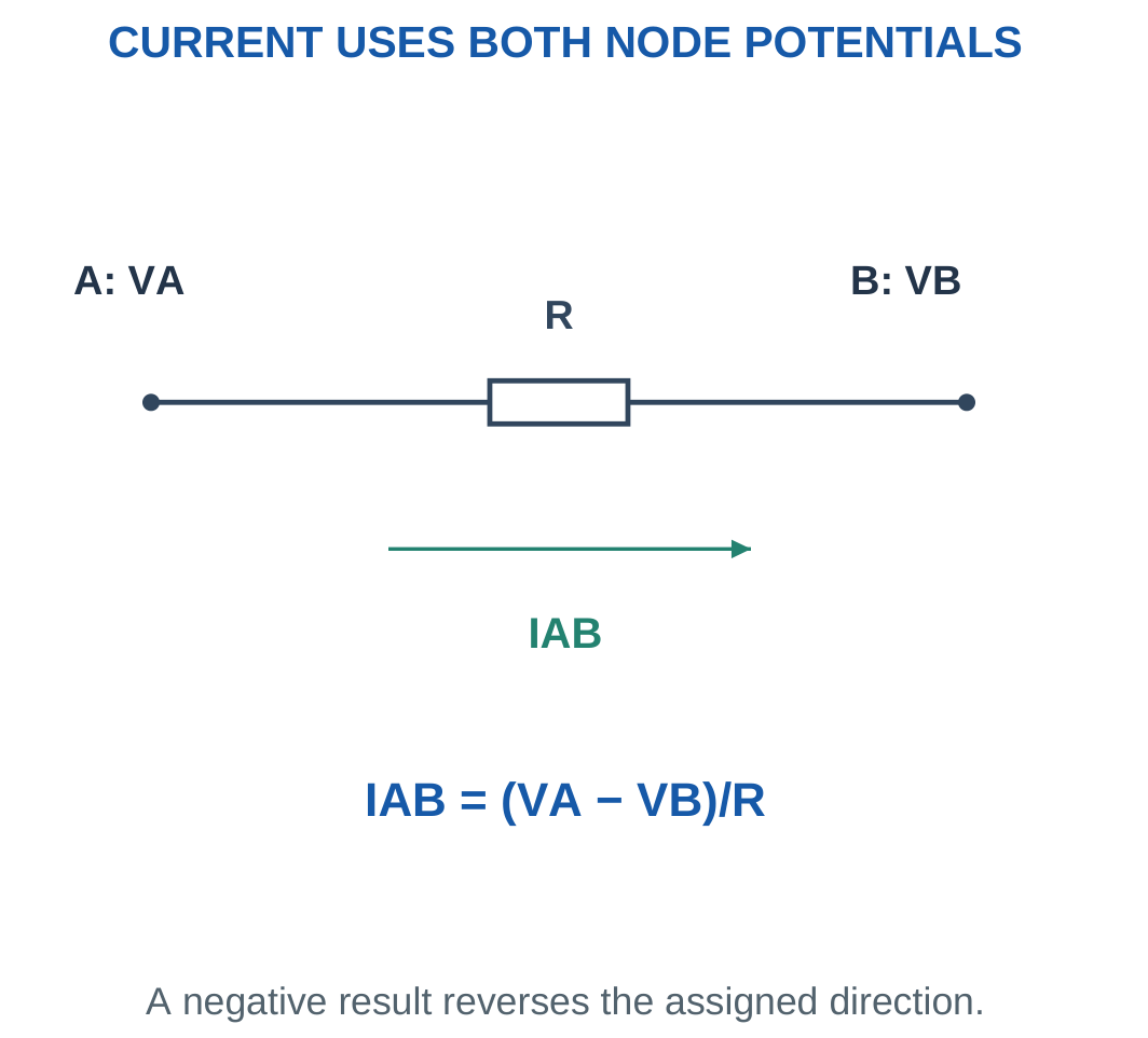
Resistor power remains:
P = IAB²R
It is independent of the arbitrary arrow direction because the current is squared.
A negative node voltage means the node is below the chosen reference. A negative branch current means current opposes the chosen arrow. Neither result should be rejected solely because it is negative.
Distinguish Quantities
A negative resistor voltage paired with a negative passive-reference current still gives positive absorbed power.
Signs describe references. A positive resistor does not become an energy source merely because one reference variable is negative.
Worked Problem 1.67: Positive A-to-B Current
Problem: VA = 8 V, VB = 2 V and R = 3 Ω.
IAB = (8 − 2)/3.
IAB = 2 A.
P = 2² × 3.
P = 12 W.
Current flows from A toward B because A has the higher potential.
Worked Problem 1.68: Negative A-to-B Current
Problem: VA = 1 V, VB = 5 V and R = 2 Ω.
IAB = (1 − 5)/2.
IAB = −2 A.
Actual current is 2 A from B toward A.
P = (−2)² × 2.
P = 8 W.
Worked Problem 1.69: A Negative Node Potential
Problem: VA = −3 V, VB = 1 V and R = 1000 Ω.
IAB = (−3 − 1)/1000.
IAB = −4 mA.
Actual current is 4 mA from B to A.
P = 0.004² × 1000.
P = 0.016 W = 16 mW.
23. Nodal Analysis: Systematic Procedure
Nodal analysis finds node potentials relative to a chosen reference using KCL and component voltage-current relations.
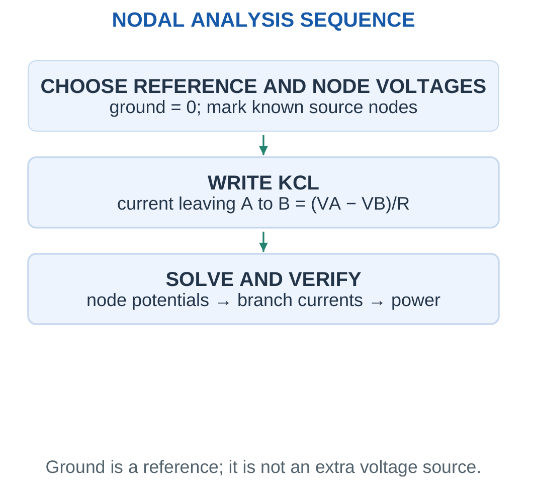
The procedure is:
- Choose a convenient reference node.
- Label all other node potentials.
- Identify any potentials fixed directly by ideal voltage sources.
- Write KCL at each unknown node.
- Express resistor currents using actual terminal differences.
- Solve the resulting linear equations.
- Recover requested branch currents, voltages and powers.
- Check signed KCL and power balance.

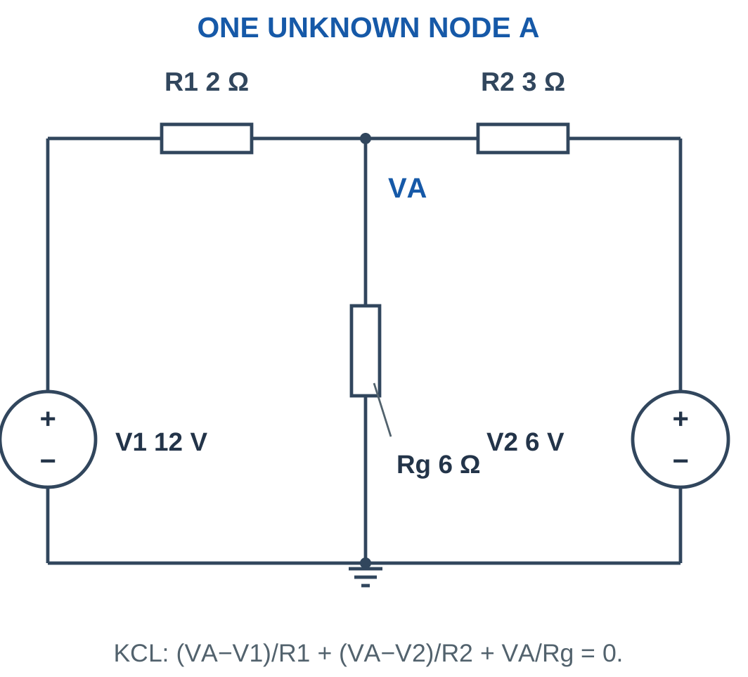
For an unknown node A connected to known potentials V1 and V2 and to ground:
(VA − V1)/R1 + (VA − V2)/R2 + VA/Rg = 0
This is an all-leaving-current equation.
A source connected directly between a node and reference can fix that node potential immediately. More complicated source placements may require supernode analysis, which is beyond the simple introductory networks considered here.
Equation Check
Every resistor term needs the starting-node potential minus the ending-node potential.
Writing VA/R for every branch is correct only when every other endpoint is actually ground.
Worked Problem 1.70: Build One KCL Equation
Problem: A connects through 2 Ω to 12 V, through 3 Ω to 6 V and through 6 Ω to ground.
KCL:
(VA − 12)/2 + (VA − 6)/3 + VA/6 = 0.
Multiply by 6:
3VA − 36 + 2VA − 12 + VA = 0.
6VA − 48 = 0.
VA = 8 V.
Leaving currents are −2 A, 2/3 A and 4/3 A. Their sum is zero.
24. One-Unknown-Node Voltage-Source Networks
For an unknown node connected through positive resistors to known potentials:
VAΣ(1/Ri) = Σ(Vi/Ri).
Therefore:
VA = Σ(Vi/Ri)/Σ(1/Ri)
A branch connected to ground has Vi = 0.

The result is a conductance-weighted average of the connected known potentials when the network contains only positive resistors at that unknown node.
Consequently, VA lies between the smallest and largest known connected potentials. A current source or another additional element can change this bound, so the condition must be checked before using it.
After finding VA, calculate every requested branch current. A lower-voltage source may receive current while a higher-voltage source delivers current.
Efficient Working
Using kΩ with mA is convenient for small networks. The same equation works in base SI units, but every term must use a consistent scale.
Do not stop at a node potential when the problem asks for branch current or load power.
Worked Problem 1.71: One-Node Network

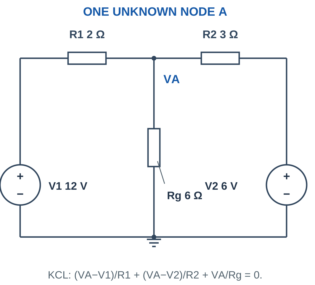
Problem: R1 = 2 Ω to V1 = 12 V, R2 = 3 Ω to V2 = 6 V and Rg = 6 Ω to ground.
VA(1/2 + 1/3 + 1/6) = 12/2 + 6/3.
VA × 1 = 8.
VA = 8 V.
Currents leaving A:
- Toward 12 V: (8 − 12)/2 = −2 A.
- Toward 6 V: (8 − 6)/3 = 0.6667 A.
- Toward ground: 8/6 = 1.3333 A.
Their signed sum is zero.
Worked Problem 1.72: A 10 V and 5 V Network


Problem: R1 = 5 Ω to 10 V, R2 = 5 Ω to 5 V and Rg = 10 Ω to ground.
VA(1/5 + 1/5 + 1/10) = 10/5 + 5/5.
0.5VA = 3.
VA = 6 V.
Leaving currents are:
−0.8 A, 0.2 A and 0.6 A.
The current from the 10 V source enters the node and divides between the other paths.
Worked Problem 1.73: A 24 V and 12 V Network

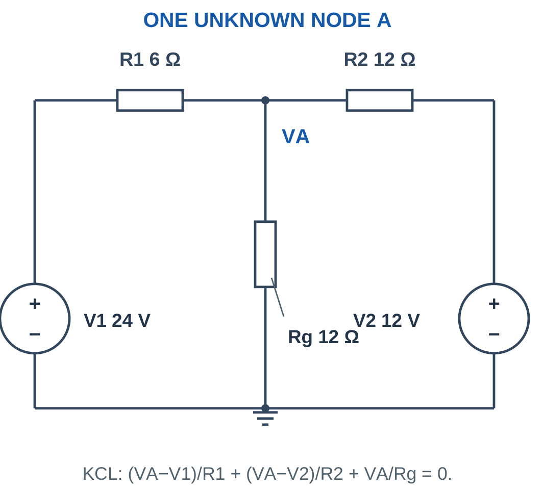
Problem: R1 = 6 Ω to 24 V, R2 = 12 Ω to 12 V and Rg = 12 Ω to ground.
VA(1/6 + 1/12 + 1/12) = 24/6 + 12/12.
VA/3 = 5.
VA = 15 V.
Leaving currents:
- Toward 24 V: −1.5 A.
- Toward 12 V: 0.25 A.
- Toward ground: 1.25 A.
These currents balance exactly before rounding.
Worked Problem 1.74: A Negative Known Potential

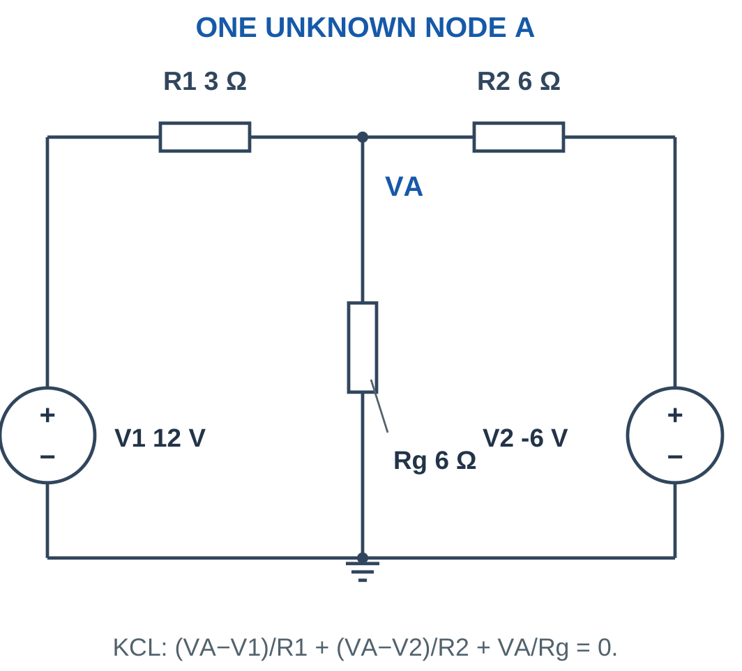
Problem: R1 = 3 Ω to 12 V, R2 = 6 Ω to −6 V and Rg = 6 Ω to ground.
VA(1/3 + 1/6 + 1/6) = 12/3 + (−6)/6.
(2/3)VA = 3.
VA = 4.5 V.
Leaving currents:
- To 12 V: (4.5 − 12)/3 = −2.5 A.
- To −6 V: (4.5 + 6)/6 = 1.75 A.
- To ground: 4.5/6 = 0.75 A.
−2.5 + 1.75 + 0.75 = 0.
Worked Problem 1.75: A Kilohm One-Node Network


Problem: R1 = 1 kΩ to 5 V, R2 = 2 kΩ to 0 V and Rg = 2 kΩ to ground.
Using kΩ and mA:
VA(1 + 1/2 + 1/2) = 5.
2VA = 5.
VA = 2.5 V.
Leaving currents are:
−2.5 mA, 1.25 mA and 1.25 mA.
25. Two-Node Nodal Analysis
When two node potentials are unknown, write one independent KCL equation at each node and solve the pair simultaneously.
A resistor Rm between A and B contributes:
(VA − VB)/Rm
to the all-leaving equation at A and:
(VB − VA)/Rm
to the all-leaving equation at B.
These terms are equal and opposite.


For a ladder with Vs through R1 to A, R2 from A to ground, R3 from A to B and R4 from B to ground:
(VA − Vs)/R1 + VA/R2 + (VA − VB)/R3 = 0
(VB − VA)/R3 + VB/R4 = 0
Solve by substitution, elimination or a clearly specified matrix method.
The B equation can often be rearranged as:
VB = [R4/(R3 + R4)]VA
This also follows from the unloaded divider formed by R3 and R4 relative to node A.
Do Not Stop Early
Node voltages are intermediate quantities when the requested answer is load current or power.
For R4 connected from B to ground:
I4 = VB/R4
P4 = VB²/R4
Use the actual resistor voltage rather than automatically using VA or the source voltage.
Worked Problem 1.76: Two-Node Resistor Ladder

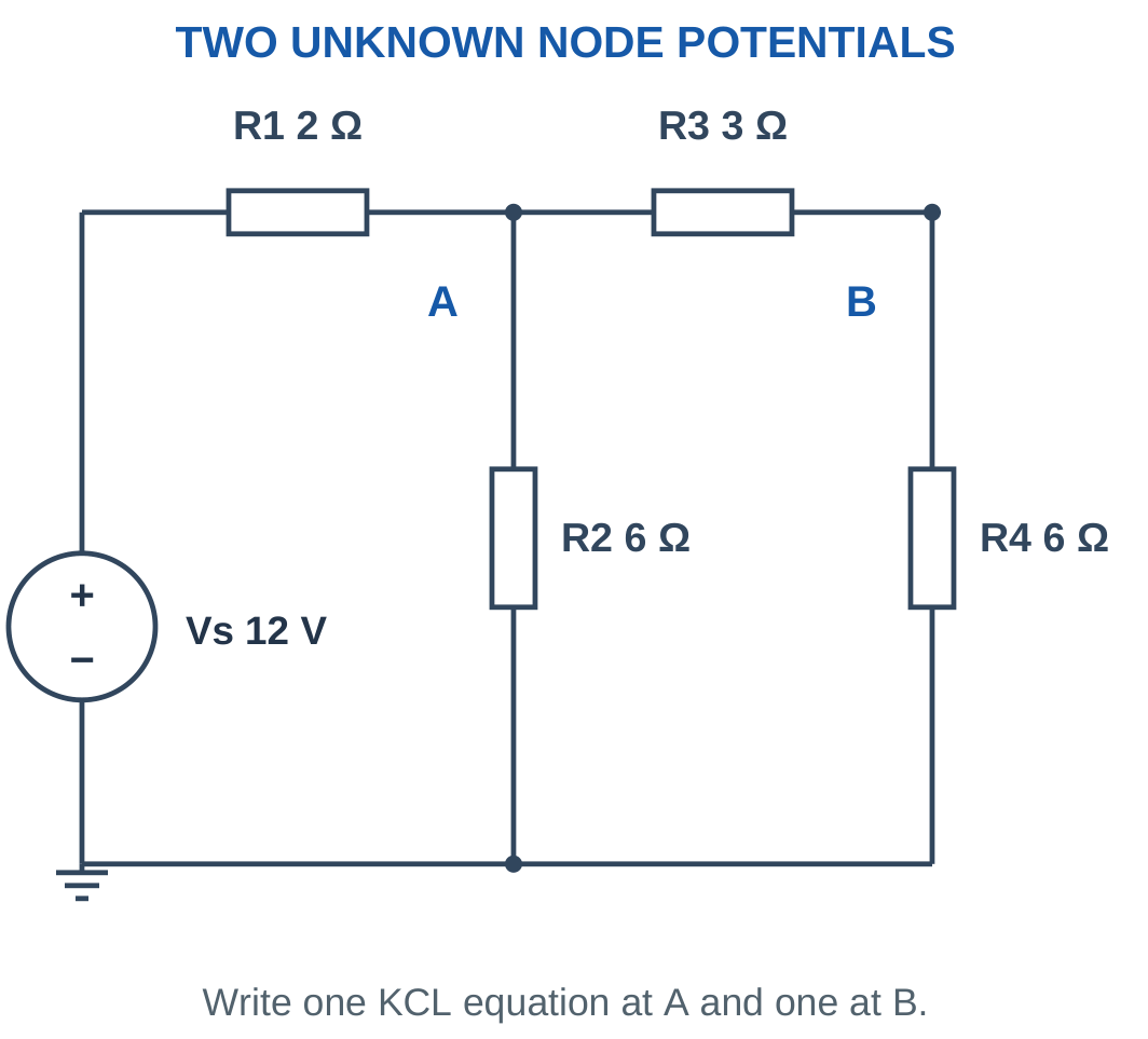
Problem: Vs = 12 V, R1 = 2 Ω, R2 = 6 Ω, R3 = 3 Ω and R4 = 6 Ω.
At A:
(VA − 12)/2 + VA/6 + (VA − VB)/3 = 0.
At B:
(VB − VA)/3 + VB/6 = 0.
The second equation gives:
VB = (6/9)VA = (2/3)VA.
Substitute into the A equation:
[1/2 + 1/6 + 1/9]VA = 6.
VA ≈ 7.7143 V.
VB ≈ 5.1429 V.
Load current:
I4 = 5.1429/6.
I4 ≈ 0.8571 A.
Source current:
Is = (12 − 7.7143)/2.
Is ≈ 2.1429 A.
Worked Problem 1.77: A Scaled Ladder

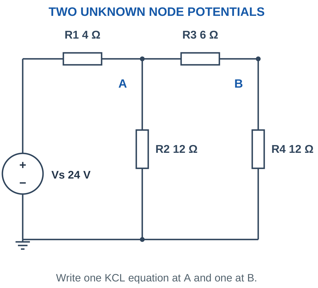
Problem: Vs = 24 V, R1 = 4 Ω, R2 = 12 Ω, R3 = 6 Ω and R4 = 12 Ω.
At A:
(VA − 24)/4 + VA/12 + (VA − VB)/6 = 0.
At B:
(VB − VA)/6 + VB/12 = 0.
Therefore:
VB = (12/18)VA = (2/3)VA.
Substitution gives:
[1/4 + 1/12 + 1/18]VA = 6.
VA ≈ 15.4286 V.
VB ≈ 10.2857 V.
I4 = VB/12.
I4 ≈ 0.8571 A.
Source current:
Is ≈ 2.1429 A.
The node voltages double relative to the previous example while the relevant resistance values also double, preserving the currents.
Worked Problem 1.78: Kilohm Ladder

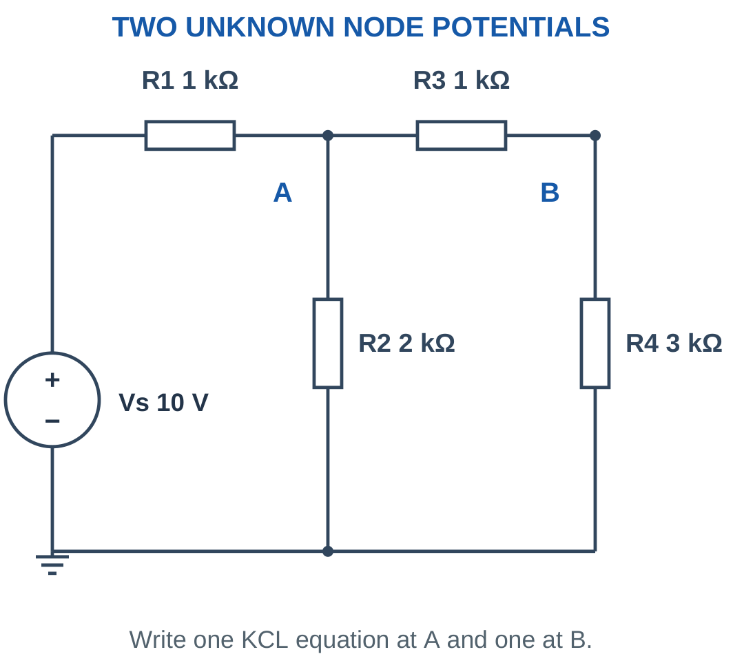
Problem: Vs = 10 V, R1 = 1 kΩ, R2 = 2 kΩ, R3 = 1 kΩ and R4 = 3 kΩ.
Using kΩ:
(VA − 10)/1 + VA/2 + (VA − VB)/1 = 0.
(VB − VA)/1 + VB/3 = 0.
The B equation gives:
VB = (3/4)VA.
Substituting:
[1 + 1/2 + 1/4]VA = 10.
VA ≈ 5.7143 V.
VB ≈ 4.2857 V.
I4 = 4.2857/3.
I4 ≈ 1.42857 mA.
Source current:
Is = (10 − 5.7143)/1.
Is ≈ 4.28571 mA.
Worked Problem 1.79: A Second Two-Node Ladder

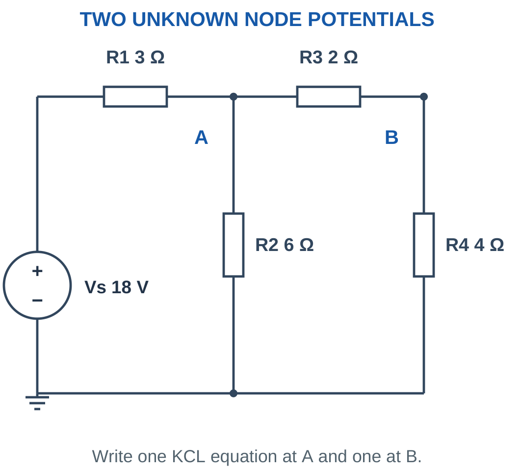
Problem: Vs = 18 V, R1 = 3 Ω, R2 = 6 Ω, R3 = 2 Ω and R4 = 4 Ω.
At A:
(VA − 18)/3 + VA/6 + (VA − VB)/2 = 0.
At B:
(VB − VA)/2 + VB/4 = 0.
Therefore:
VB = (4/6)VA = (2/3)VA.
Substitution gives:
[1/3 + 1/6 + 1/6]VA = 6.
VA = 9 V.
VB = 6 V.
I4 = 6/4.
I4 = 1.5 A.
Source current:
Is = (18 − 9)/3.
Is = 3 A.
The current through R2 is 9/6 = 1.5 A, so source current divides equally between the grounded R2 branch and the R3–R4 path.
26. Nodal Analysis with Current Injection
An ideal current source fixes its branch current in the arrow direction. The surrounding network determines the voltage needed to support that current.
For a source injecting Is into a node connected to grounded resistors R1 and R2:
Is = VA/R1 + VA/R2.
Therefore:
VA = Is(R1 || R2)

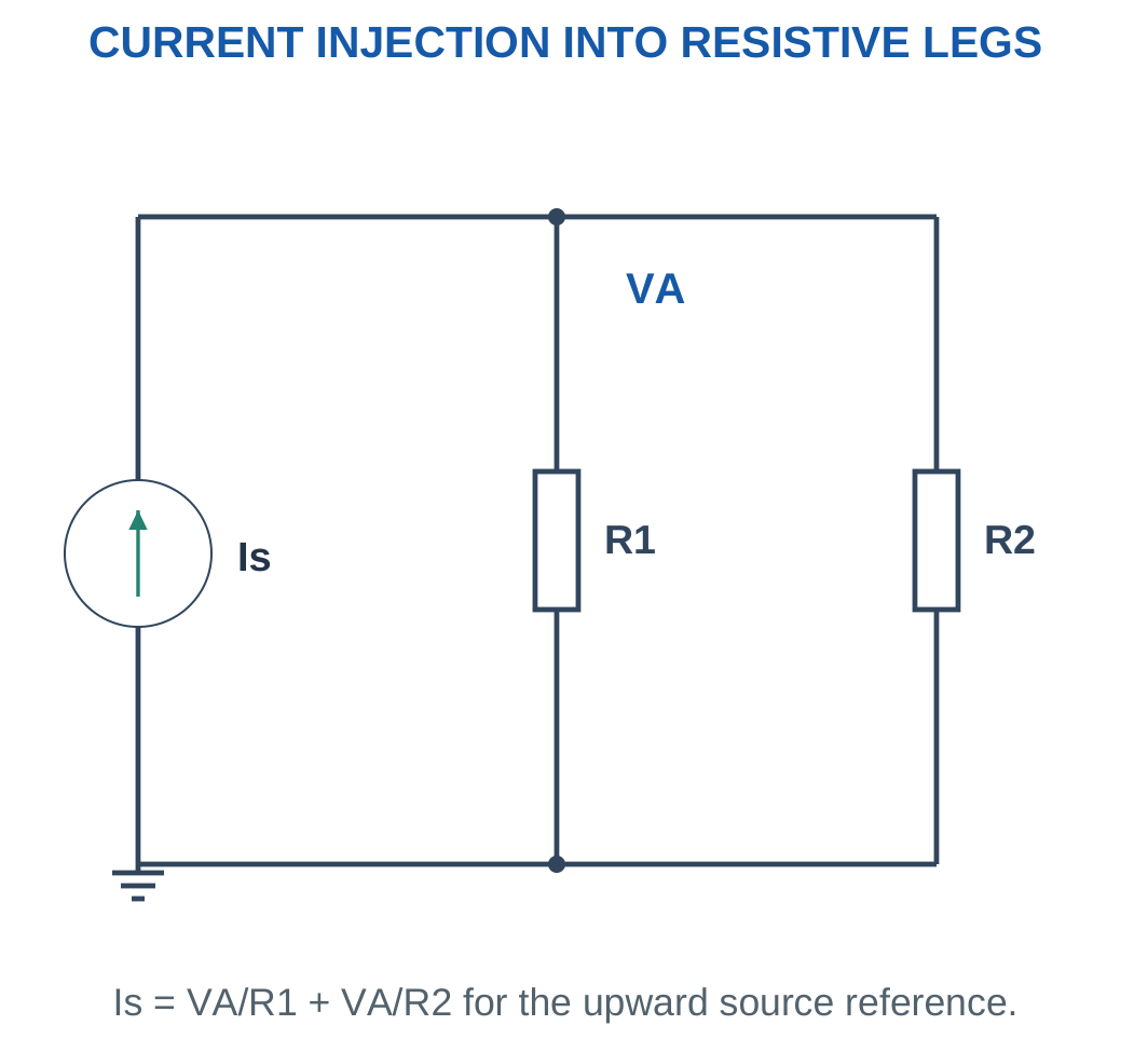
If the source arrow is reversed, its injection is negative in the same KCL convention.
The node voltage can become negative without violating the passive nature of positive resistors. The actual resistor currents then flow from reference toward the negative node.
An ideal current source develops the voltage required by the mathematical model. Real current sources have compliance limits, but no additional voltage should be invented when only an ideal current is specified.
Power Check
For a positive injection raising the node above ground, the ideal current source delivers power while the grounded resistors absorb it.
The total resistor dissipation should equal the magnitude of source-delivered power.
Worked Problem 1.80: Current-Source Node Voltage
Problem: A source injects 3 A into A. Resistors 6 Ω and 3 Ω connect A to ground.
Rp = 6 || 3.
Rp = 2 Ω.
VA = 3 × 2.
VA = 6 V.
Downward currents:
I1 = 6/6.
I1 = 1 A.
I2 = 6/3.
I2 = 2 A.
The two currents add to the 3 A injection.
Worked Problem 1.81: A Milliampere Injection
Problem: Is = 12 mA, R1 = 1 kΩ and R2 = 2 kΩ.
Rp = (1 × 2)/(1 + 2).
Rp = 0.6666667 kΩ.
VA = 12 mA × 0.6666667 kΩ.
VA = 8 V.
Downward currents:
I1 = 8 mA.
I2 = 4 mA.
Worked Problem 1.82: Negative Injection
Problem: Signed injection is −2 A into A. Both grounded resistors are 4 Ω.
Rp = 4 || 4.
Rp = 2 Ω.
VA = −2 × 2.
VA = −4 V.
Each downward reference current is:
I = −4/4.
I = −1 A.
The physical current in each resistor is 1 A upward from ground toward A.
27. Mesh Analysis and Shared Resistance
Mesh analysis uses KVL with independent mesh-current variables for a planar network.
Assign a direction to each mesh, commonly clockwise.
A resistor belonging only to mesh 1 carries I1. A resistor shared by two clockwise meshes usually carries the difference of the two mesh currents in a chosen branch direction.
If downward through the shared resistor follows mesh 1:
Ishared = I1 − I2

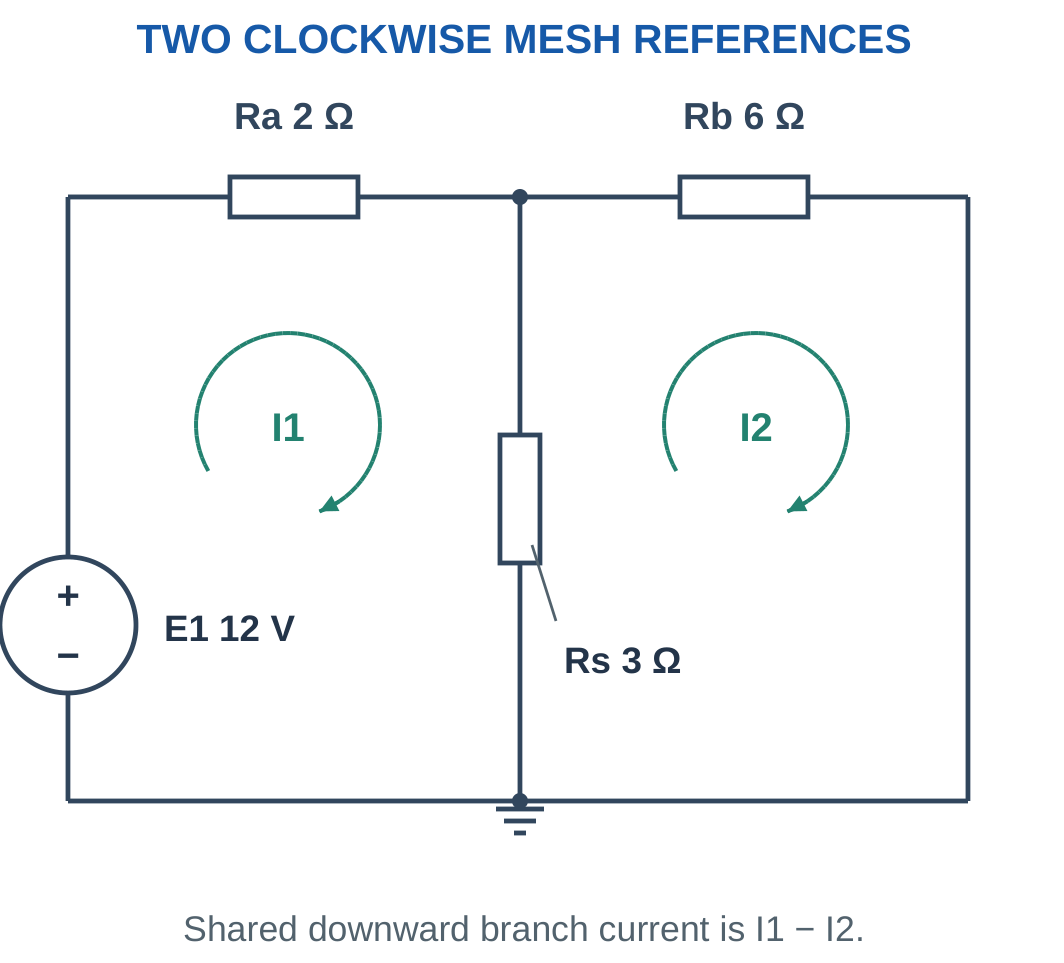
The coefficient multiplying a mesh’s own current is the sum of resistances around that mesh.
A shared resistor contributes a negative coefficient for the neighbouring clockwise mesh current.
The source term depends on traversal through its marked polarity.
After solving, convert mesh variables into actual requested branch currents. Mesh currents are mathematical variables used to reconstruct physical branch currents.
Essential Distinction
A shared resistor does not automatically carry I1 or I2 alone. Equal clockwise mesh currents can produce zero current in their common branch.
Worked Problem 1.83: Shared Branch Current
Problem: I1 = 2 A and I2 = 0.75 A, both clockwise. The shared resistor is 4 Ω, with downward reference following mesh 1.
Ishared = 2 − 0.75.
Ishared = 1.25 A downward.
Vdown = IsharedR.
Vdown = 1.25 × 4.
Vdown = 5 V.
P = 1.25² × 4.
P = 6.25 W.
Using 2² × 4 would overestimate power because 2 A is a mesh variable, not the actual shared-branch current.
28. Two-Mesh Networks with One Source
Consider a left source E rising upward, outer resistors Ra and Rb and shared resistor Rs.
With two clockwise mesh currents:
(Ra + Rs)I1 − RsI2 = E
−RsI1 + (Rb + Rs)I2 = 0

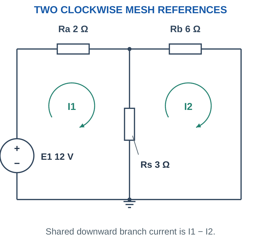
The shared downward current is:
Ishared = I1 − I2
The source branch carries I1. The outer right resistor carries I2 in its assigned mesh direction.
For this one-source circuit, power balance is:
EI1 = RaI1² + RbI2² + Rs(I1 − I2)²
This network can also be solved by reducing Rs parallel to Rb, then adding Ra in series. Reduction provides an independent check on the mesh equations.
Interpretation
A mesh current is a mathematical loop variable. It is not an additional physical current circulating alongside the branch currents.
The branch current is the algebraic sum of mesh contributions that pass through that branch.
Worked Problem 1.84: One-Source Two-Mesh Circuit

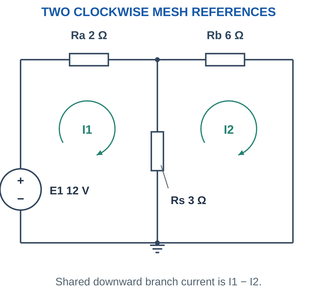
Problem: E = 12 V, Ra = 2 Ω, Rb = 6 Ω and Rs = 3 Ω.
Mesh equations:
5I1 − 3I2 = 12.
−3I1 + 9I2 = 0.
From the second:
I2 = I1/3.
Substitute:
5I1 − I1 = 12.
I1 = 3 A.
I2 = 1 A.
Ishared = 3 − 1.
Ishared = 2 A downward.
Centre-node voltage:
V = 2 × 3.
V = 6 V.
Worked Problem 1.85: A 24 V Mesh Circuit

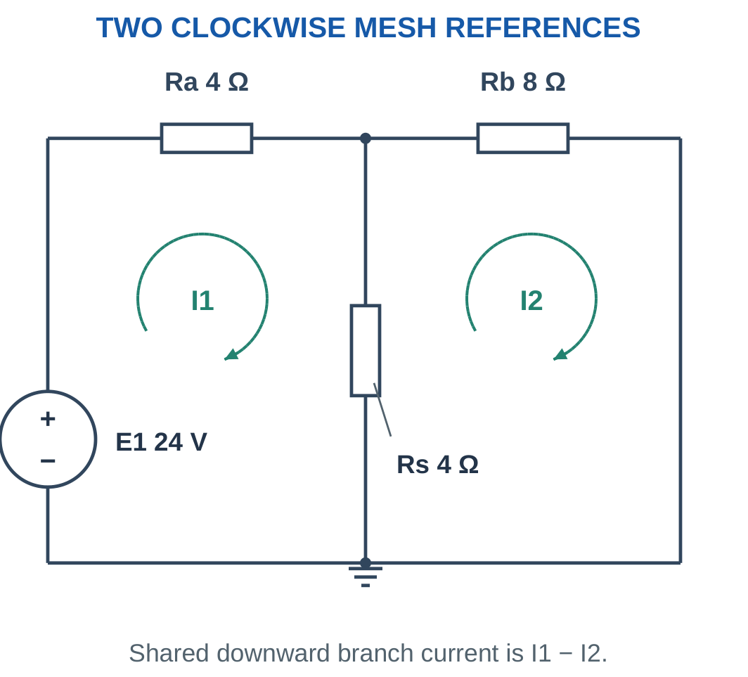
Problem: E = 24 V, Ra = 4 Ω, Rb = 8 Ω and Rs = 4 Ω.
8I1 − 4I2 = 24.
−4I1 + 12I2 = 0.
I2 = I1/3.
Substitute:
8I1 − (4/3)I1 = 24.
I1 = 3.6 A.
I2 = 1.2 A.
Ishared = 3.6 − 1.2.
Ishared = 2.4 A.
Centre voltage:
V = 2.4 × 4.
V = 9.6 V.
Worked Problem 1.86: Mesh Currents in Milliamperes

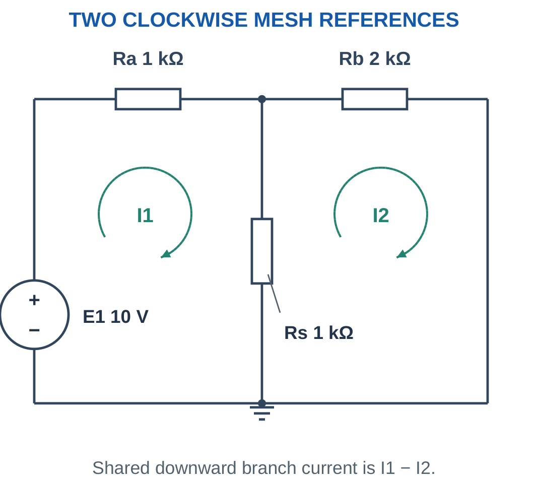
Problem: E = 10 V, Ra = 1 kΩ, Rb = 2 kΩ and Rs = 1 kΩ.
Using kΩ and mA:
2I1 − I2 = 10.
−I1 + 3I2 = 0.
I2 = I1/3.
Substitute:
2I1 − I1/3 = 10.
I1 = 6 mA.
I2 = 2 mA.
Ishared = 4 mA.
Centre-node voltage:
V = 4 mA × 1 kΩ.
V = 4 V.
Worked Problem 1.87: A Second One-Source Network

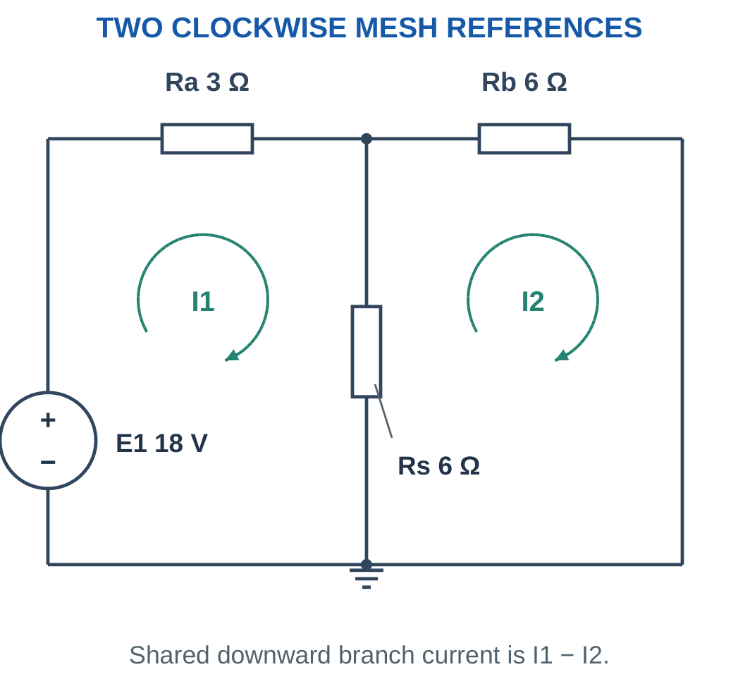
Problem: E = 18 V, Ra = 3 Ω, Rb = 6 Ω and Rs = 6 Ω.
9I1 − 6I2 = 18.
−6I1 + 12I2 = 0.
I2 = I1/2.
Substitute:
9I1 − 3I1 = 18.
I1 = 3 A.
I2 = 1.5 A.
Ishared = 1.5 A.
Centre voltage:
V = 1.5 × 6.
V = 9 V.
29. Two-Source Networks and Negative Mesh Values
A second source changes the right-hand side of the mesh equations according to its polarity.
When both source top terminals are positive, a clockwise traversal through the right source crosses it from positive to negative. Its contribution is a drop.
The equations become:
(Ra + Rs)I1 − RsI2 = E1
−RsI1 + (Rb + Rs)I2 = −E2

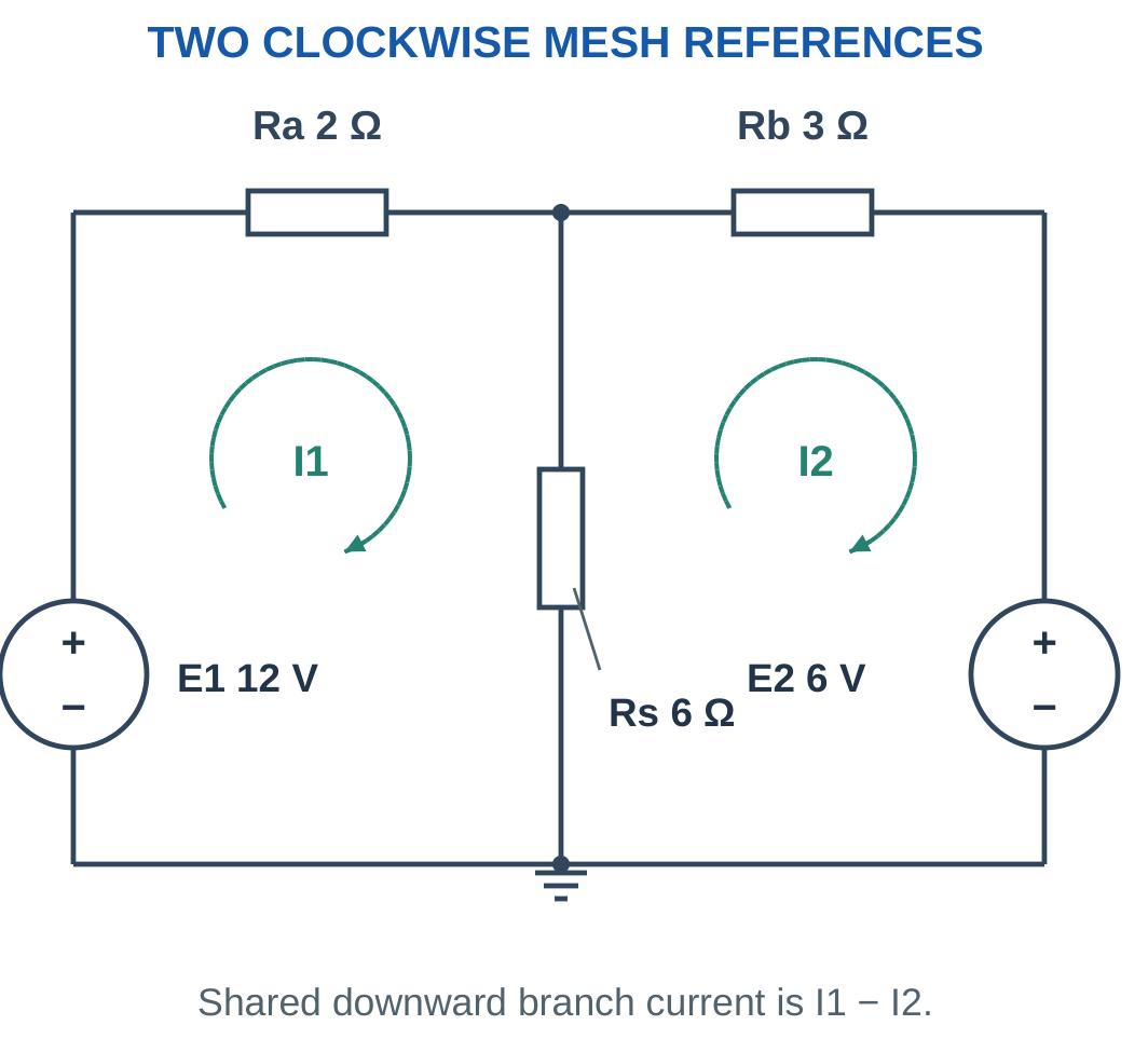
A negative I2 means actual current in the right outer branch is opposite the assigned clockwise reference.
Compute source power using the actual branch current direction and source polarity. A source can absorb energy in the ideal model.
The centre-node voltage from mesh analysis must agree with a nodal calculation of the same circuit.
Sign Cue
A source is not negative merely because it appears on the right side of a drawing. Its equation sign follows the marked terminals and selected traversal.
Worked Problem 1.88: Two Sources with Explicit Polarity


Problem: E1 = 12 V, E2 = 6 V, Ra = 2 Ω, Rb = 3 Ω and Rs = 6 Ω.
Equations:
8I1 − 6I2 = 12.
−6I1 + 9I2 = −6.
From the second:
I2 = (6I1 − 6)/9.
Substitution gives:
8I1 − 6(6I1 − 6)/9 = 12.
I1 = 2 A.
I2 ≈ 0.6667 A.
Shared downward current:
Ishared ≈ 1.3333 A.
Centre potential:
V = 6 × 1.3333.
V = 8 V.
Worked Problem 1.89: A Negative Right Mesh Current

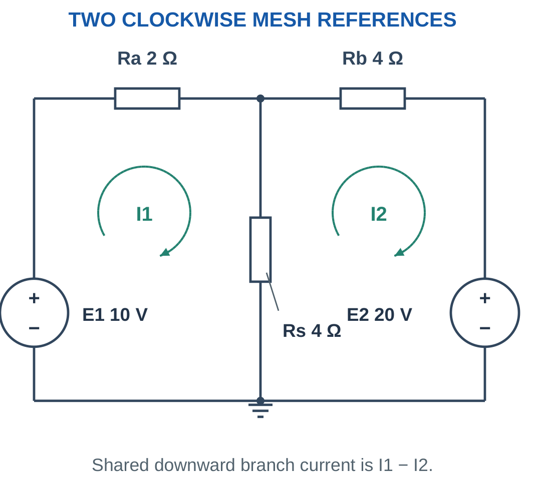
Problem: E1 = 10 V, E2 = 20 V, Ra = 2 Ω, Rb = 4 Ω and Rs = 4 Ω.
6I1 − 4I2 = 10.
−4I1 + 8I2 = −20.
From the second:
I2 = 0.5I1 − 2.5.
Substitute:
6I1 − 4(0.5I1 − 2.5) = 10.
4I1 + 10 = 10.
I1 = 0 A.
I2 = −2.5 A.
Shared current:
Ishared = 0 − (−2.5).
Ishared = 2.5 A downward.
Centre voltage:
V = 2.5 × 4.
V = 10 V.
The left source has nonzero voltage but zero current, so its power is zero in this operating condition.
Worked Problem 1.90: Unequal Sources and Resistors

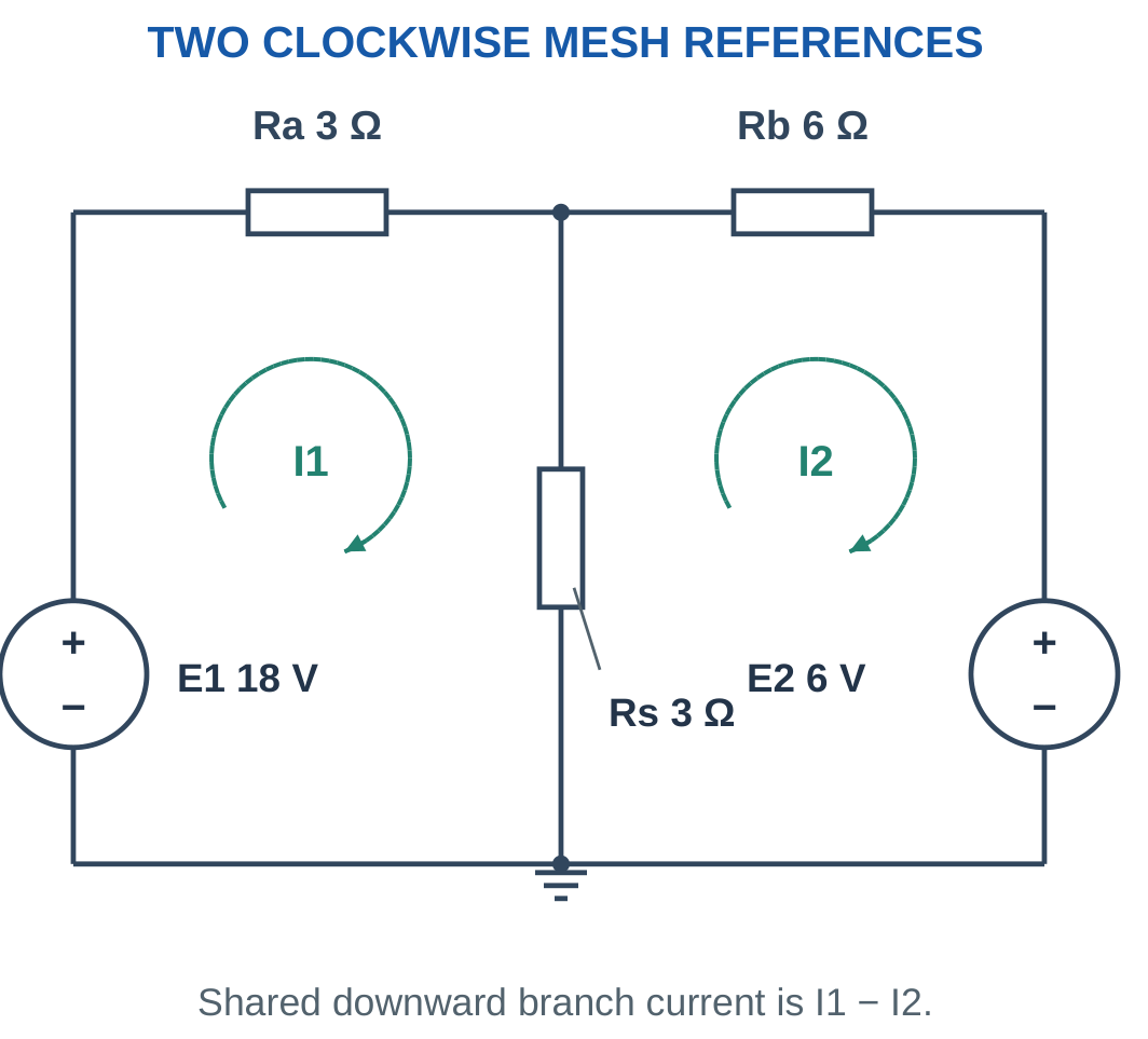
Problem: E1 = 18 V, E2 = 6 V, Ra = 3 Ω, Rb = 6 Ω and Rs = 3 Ω.
6I1 − 3I2 = 18.
−3I1 + 9I2 = −6.
From the second:
I2 = (3I1 − 6)/9.
Substitute into the first equation.
I1 = 3.2 A.
I2 = 0.4 A.
Ishared = 3.2 − 0.4.
Ishared = 2.8 A.
Centre potential:
V = 2.8 × 3.
V = 8.4 V.
Worked Problem 1.91: Symmetric Two-Source Network

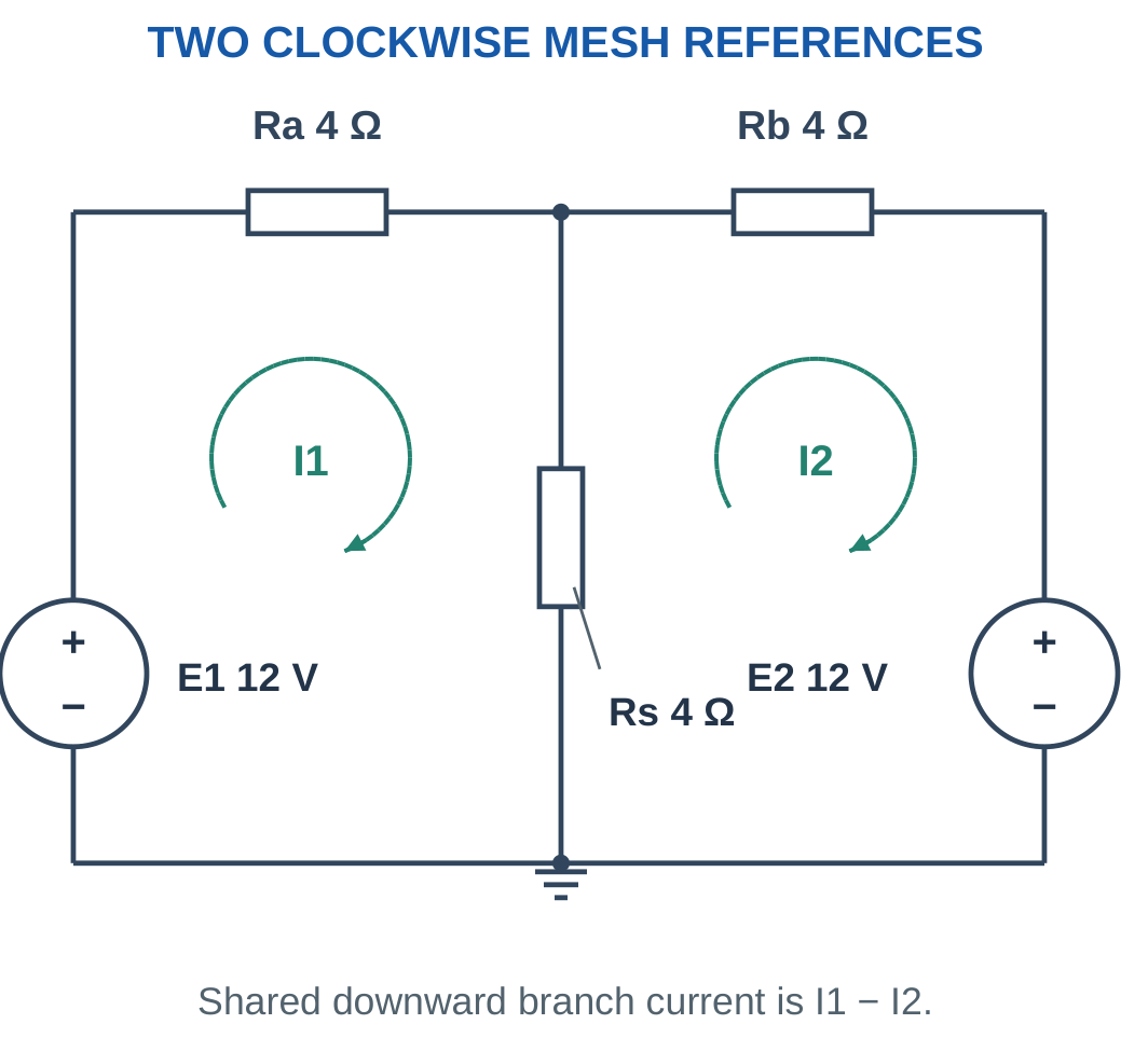
Problem: E1 = E2 = 12 V and Ra = Rb = Rs = 4 Ω.
8I1 − 4I2 = 12.
−4I1 + 8I2 = −12.
Solving:
I1 = 1 A.
I2 = −1 A.
Shared downward current:
Ishared = 1 − (−1).
Ishared = 2 A.
Centre voltage:
V = 2 × 4.
V = 8 V.
Both sources supply current toward the centre node in the physical circuit, while their clockwise mesh references have opposite signs.
30. Choosing and Cross-Checking an Analysis Method
Use direct series and parallel reduction when the topology clearly permits it.
Nodal analysis is often concise when few node potentials are unknown or current injections are specified.
Mesh analysis is often convenient for a planar network containing a small number of loops and voltage sources.

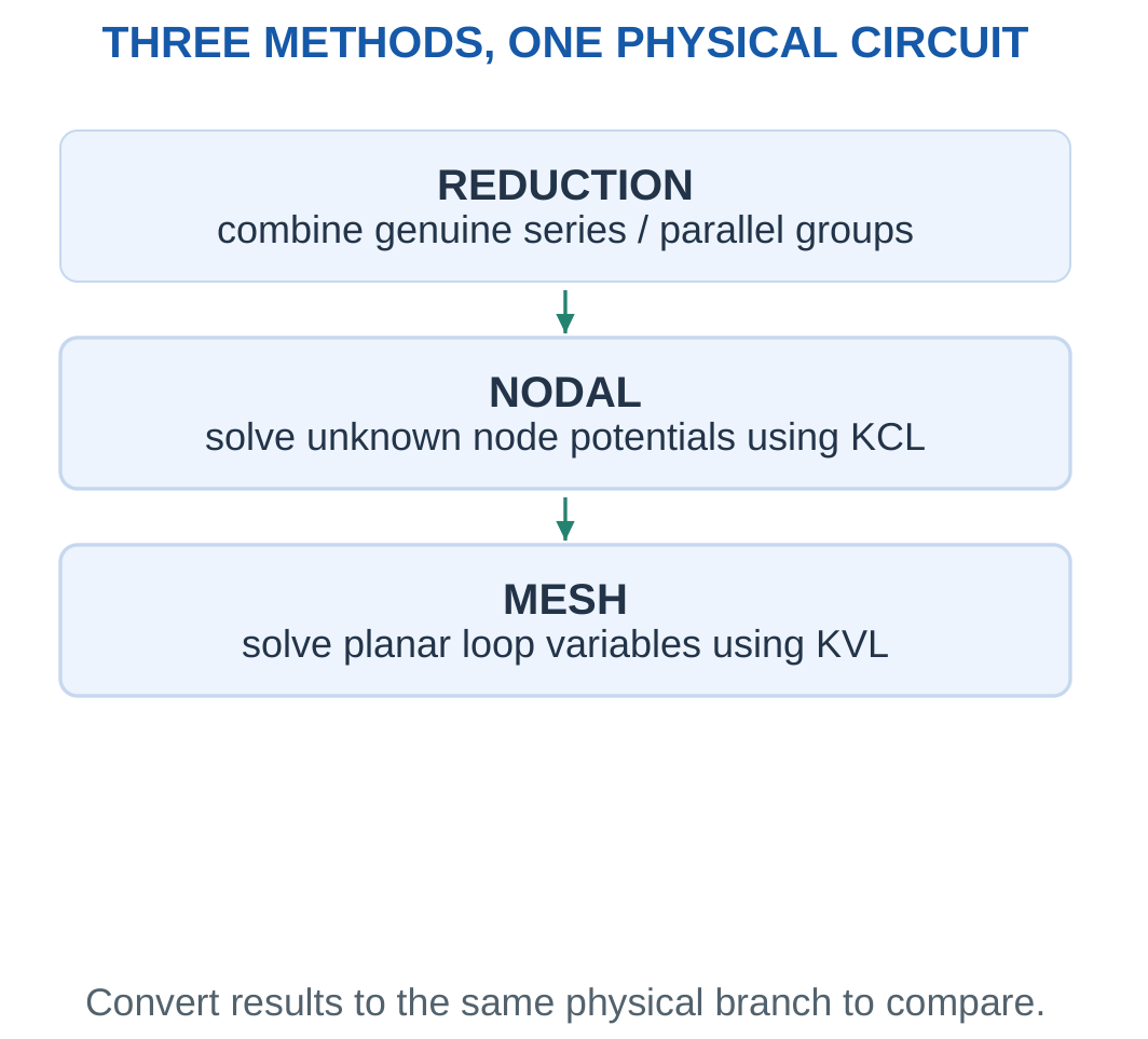
A short equation set is useful, but correctness depends on maintaining topology and references.
When an examination asks for a particular method, show that method even if another gives a quick private check.
Do not compare a mesh variable directly with a branch current without accounting for shared elements.
KCL, KVL and power balance detect different mistakes. A missing node branch, reversed source polarity, incorrect shared-current expression and lost unit prefix may produce different patterns of failed checks.
Good Presentation
Keep a labelled diagram with the assumptions. Write equations before substituting numbers. Finish with the requested quantity, unit and interpreted direction.
A correct numerical value without a clear terminal pair or current direction may still be an incomplete answer.
Worked Problem 1.92: Reduction Cross-Check of a Mesh Result
Problem: A 12 V source feeds 2 Ω in series with 6 Ω parallel to 3 Ω. Find source current and current through the 3 Ω branch.
Rp = 6 || 3.
Rp = 2 Ω.
Rt = 2 + 2.
Rt = 4 Ω.
Source current:
Is = 12/4 = 3 A.
Parallel voltage:
Vp = 3 × 2 = 6 V.
Current through 3 Ω:
I3 = 6/3 = 2 A.
Current through 6 Ω is 1 A. These agree with the one-source mesh solution.
31. Thevenin’s Theorem and Terminal Equivalence
Thevenin’s theorem replaces an eligible linear two-terminal source network with an ideal voltage source Vth in series with resistance Rth.
A load connected to those terminals receives the same voltage and current as it would in the original network under the stated model.

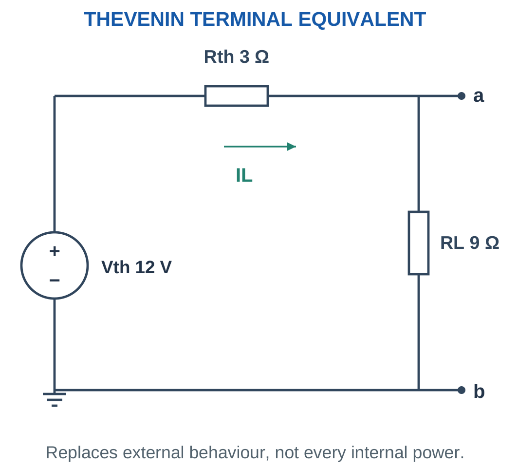
The Thevenin voltage is:
Vth = Vopen-circuit = Va − Vb
The Thevenin resistance is the resistance seen looking into the source network after independent sources are deactivated appropriately.
For the simple networks here, sources are independent and resistors are positive linear elements.
Dependent sources in advanced networks must not simply be erased. They require a suitable analysis such as a test-source method.
Thevenin equivalence preserves the external terminal relationship. It does not reproduce every internal branch current, source power or resistor temperature.
Boundary First
Mark terminals a and b and remove only the external load being studied.
Removing an internal network resistor changes the source network and can produce a different equivalent.
Worked Problem 1.93: Use a Supplied Equivalent
Problem: Vth = 12 V and Rth = 3 Ω. A 9 Ω load is connected.
IL = Vth/(Rth + RL).
IL = 12/(3 + 9).
IL = 1 A.
VL = ILRL.
VL = 9 V.
Equivalent internal drop:
VRth = 1 × 3.
VRth = 3 V.
The 9 V load voltage and 3 V internal drop add to the 12 V Thevenin voltage.
32. Finding the Open-Circuit Voltage Vth
Remove the external load while keeping independent sources active.
Calculate voltage between the marked terminals with the stated polarity.
Open circuit means the disconnected load current is zero. It does not mean every current inside the source network is zero.

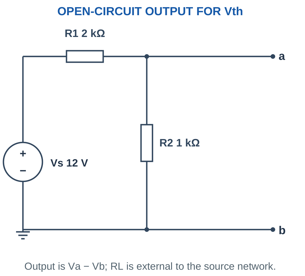
For a source divider viewed from tap to reference:
Vth = VsR2/(R1 + R2)
If a resistor R3 lies between the tap and the open output terminal, it carries zero current at open circuit. Its voltage drop is therefore zero, so it does not alter Vth in that configuration.
A more complex active network may require nodal or mesh analysis to determine open-terminal voltage.
Frequent Mistake
Independent sources remain active when finding Vth.
Source deactivation belongs to the separate Rth calculation. Turning off the source before finding Vth usually removes the very voltage being sought.
Worked Problem 1.94: Open-Circuit Divider Voltage
Problem: Vs = 12 V, R1 = 2000 Ω and R2 = 1000 Ω. Output terminals are the tap and reference.
Internal divider current:
Idivider = 12/(2000 + 1000).
Idivider = 4 mA.
Vth = IdividerR2.
Vth = 0.004 × 1000.
Vth = 4 V.
External current is zero, but internal current is 4 mA.
Worked Problem 1.95: A Low-Resistance Source Divider
Problem: Vs = 18 V, R1 = 3 Ω and R2 = 6 Ω.
Idivider = 18/(3 + 6).
Idivider = 2 A.
Vth = 2 × 6.
Vth = 12 V.
The open external terminals do not interrupt the internal series path through R1 and R2.
Worked Problem 1.96: Equal Divider Resistors
Problem: Vs = 10 V and R1 = R2 = 10 kΩ.
Idivider = 10/20,000.
Idivider = 0.5 mA.
Vth = 0.5 mA × 10 kΩ.
Vth = 5 V.
Equal divider resistors produce half the source voltage at open circuit.
33. Finding Rth and Deactivating Independent Sources
Remove the external load and deactivate independent ideal sources:
- Replace an ideal voltage source with a short circuit.
- Replace an ideal current source with an open circuit.
Then calculate resistance looking into the same terminals a and b.

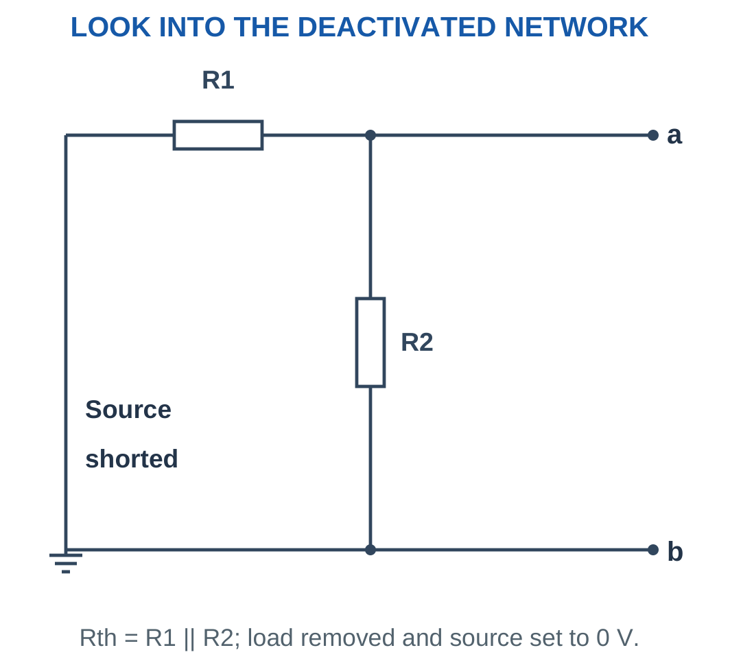
Setting an ideal voltage source to zero volts makes its terminals equipotential, equivalent to an ideal wire.
Setting an ideal current source to zero amperes prevents current through its branch, equivalent to an open.
Any explicitly modelled internal source resistance is a separate element and remains in the circuit.
For finite positive Rth and delivered output current Iout:
Vab = Vth − IoutRth
The terminal-voltage versus output-current slope is:
Slope = −Rth
Connection Check
Redraw the nodes after deactivation. Components that appeared in series in the active source network can become parallel after a voltage source is replaced by a wire.
The load itself must remain removed during the looking-in resistance calculation.
Worked Problem 1.97: Divider Resistance Seen from the Output
Problem: R1 = 2000 Ω, R2 = 1000 Ω and output series resistance R3 = 0 Ω.
Deactivate the ideal voltage source.
R1 and R2 are now parallel:
Rparallel = (2000 × 1000)/(2000 + 1000).
Rparallel = 666.6667 Ω.
Rth = R3 + Rparallel.
Rth = 666.6667 Ω.
Worked Problem 1.98: Include an Output Series Resistor
Problem: R1 = 3 Ω, R2 = 6 Ω and R3 = 2 Ω between the divider tap and output a.
R1 || R2 = (3 × 6)/(3 + 6).
R1 || R2 = 2 Ω.
Rth = R3 + (R1 || R2).
Rth = 2 + 2.
Rth = 4 Ω.
The output series resistor remains inside the source-network boundary and must be included.
Voltage-Divider Loading

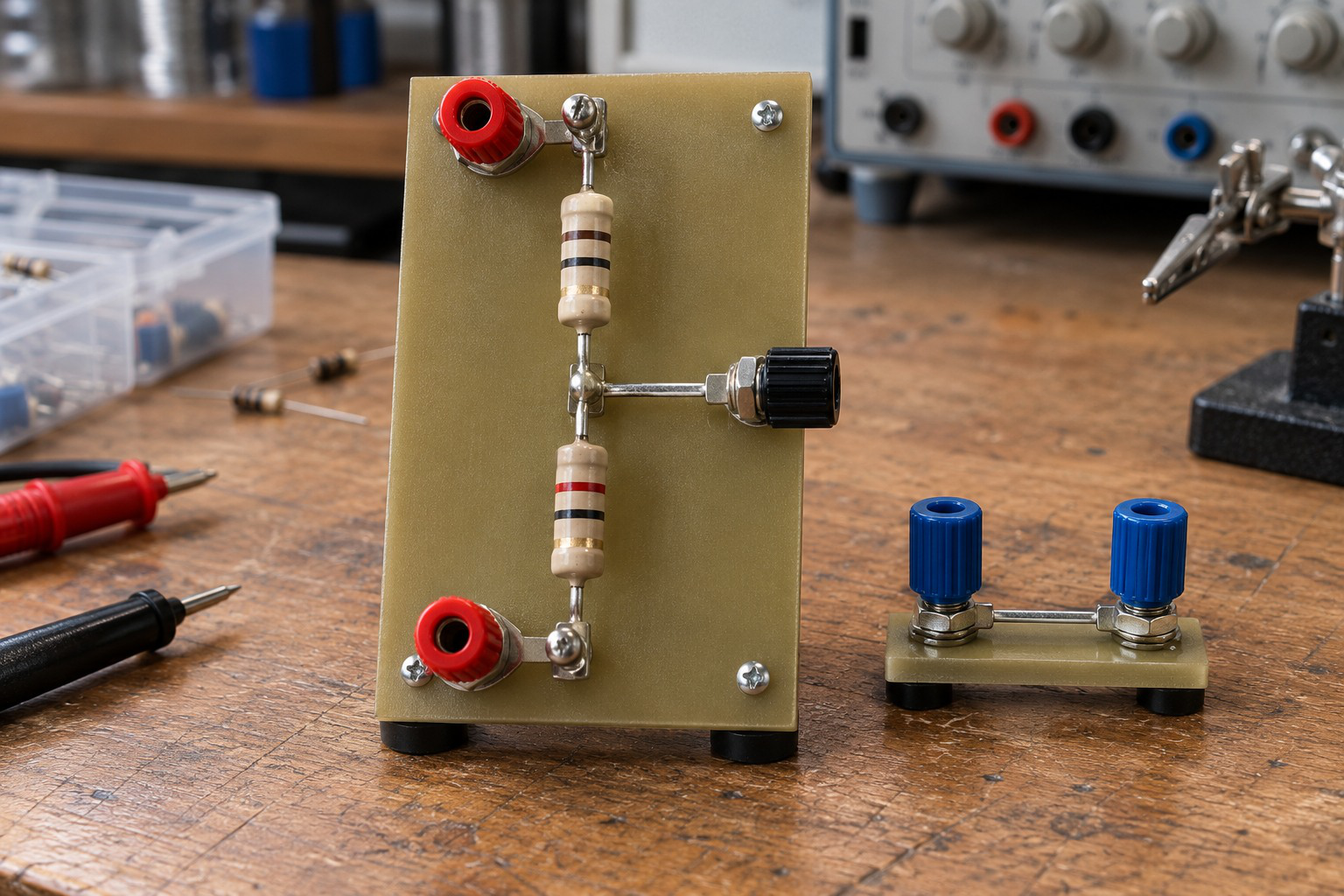
A divider ratio assumes a stated load condition. A finite input resistance can change output voltage. Identify the output port and load before using an unloaded ratio.
Thevenin resistance gives a compact way to describe how strongly that port voltage changes with load current.
34. Reconnecting the Load to the Thevenin Equivalent
After finding Vth and Rth, reconnect RL to the equivalent.
IL = Vth/(Rth + RL)
VL = ILRL
PL = IL²RL

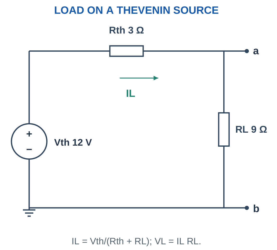
KVL gives:
Vth = ILRth + VL
A large RL draws little current, making VL close to Vth.
A small RL increases current and internal equivalent drop in the positive-resistance model.
Rth is an equivalent terminal parameter. Its I²Rth is dissipation in the equivalent representation, not automatically the original network’s total internal power.
Keep the Boundary Honest
Use the equivalent for external load behaviour.
Return to the original network when asked for a particular internal resistor current, source current or internal component power.
Worked Problem 1.99: Complete Divider Thevenin Solution
Problem: Vs = 12 V, R1 = 2000 Ω, R2 = 1000 Ω and RL = 1000 Ω.
Vth = 12 × 1000/3000.
Vth = 4 V.
Rth = 2000 || 1000.
Rth = 666.6667 Ω.
IL = 4/(666.6667 + 1000).
IL = 2.4 mA.
VL = 0.0024 × 1000.
VL = 2.4 V.
PL = 0.0024² × 1000.
PL = 0.00576 W = 5.76 mW.
Worked Problem 1.100: A Low-Resistance Load
Problem: Vs = 18 V, R1 = 3 Ω, R2 = 6 Ω and RL = 4 Ω.
Vth = 18 × 6/9.
Vth = 12 V.
Rth = 3 || 6.
Rth = 2 Ω.
IL = 12/(2 + 4).
IL = 2 A.
VL = 2 × 4.
VL = 8 V.
PL = 2² × 4.
PL = 16 W.
Worked Problem 1.101: Equal Divider and Load Values
Problem: Vs = 10 V, R1 = R2 = 10 kΩ and RL = 10 kΩ.
Vth = 5 V.
Rth = 10 kΩ || 10 kΩ.
Rth = 5 kΩ.
IL = 5/(5000 + 10,000).
IL = 0.333333 mA.
VL = 0.333333 mA × 10 kΩ.
VL ≈ 3.3333 V.
PL = IL²RL.
PL ≈ 0.00111111 W = 1.11111 mW.
A Two-Terminal Network Interface
A Thevenin model describes behaviour seen at a defined port. Open-circuit voltage and equivalent resistance have different derivations.
The number of original internal components does not determine the value of Rth. It is the network’s looking-in resistance after the correct source treatment.
35. Load Variation and Extended Thevenin Examples
Once Vth and Rth are known, several loads can be evaluated without re-solving the complete source network.
Keep the equivalent fixed while changing RL. If source values or internal connections change, find a new equivalent.

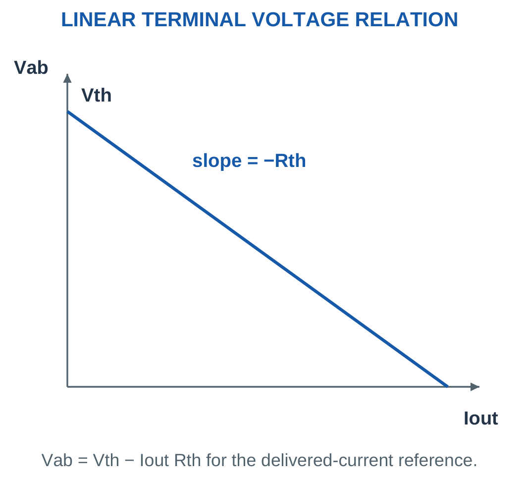
For a divider followed by output series resistor R3:
Vth = VsR2/(R1 + R2)
Rth = R3 + (R1 || R2)
R3 carries no open-circuit current, so it does not change Vth. It does carry current after load reconnection, so it affects the loaded terminal voltage.
A measured open-circuit voltage and one known loaded condition can determine a linear equivalent:
Rth = (Vth − VL)/IL
This fitted relationship applies within the assumed linear operating range.
Do Not Extrapolate Carelessly
A fitted linear source model does not establish that a real supply remains linear at arbitrary current or outside its protection limits.
The theorem simplifies the chosen model. It does not remove the need to state that model’s valid conditions.
Worked Problem 1.102: Output Series Resistance Changes Rth

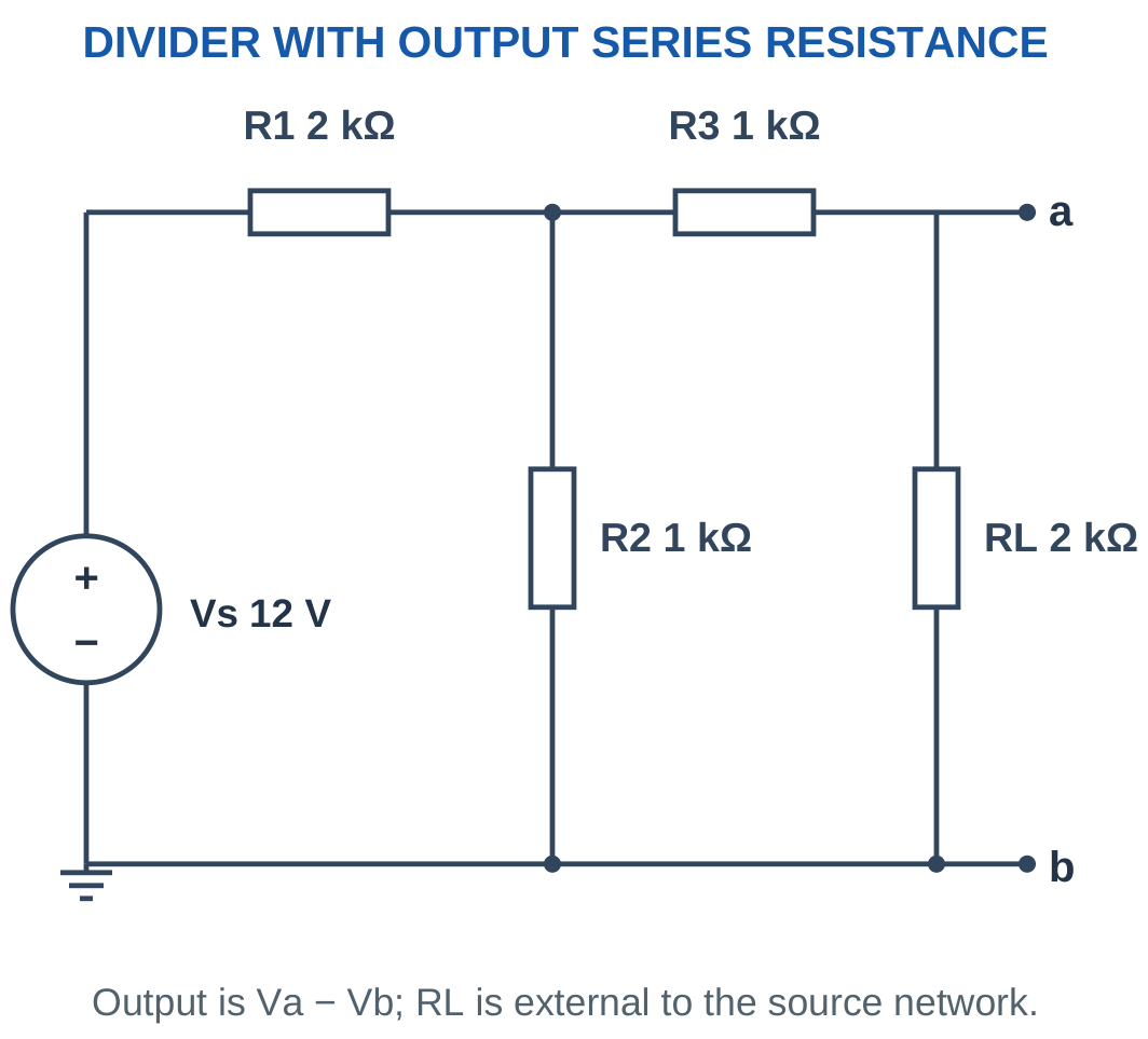
Problem: Vs = 12 V, R1 = 2000 Ω, R2 = 1000 Ω, R3 = 1000 Ω and RL = 2000 Ω.
Open-circuit voltage:
Vth = 4 V.
Parallel resistance:
R1 || R2 = 666.6667 Ω.
Rth = 1000 + 666.6667.
Rth = 1666.6667 Ω.
IL = 4/(1666.6667 + 2000).
IL ≈ 1.09091 mA.
VL = IL × 2000.
VL ≈ 2.1818 V.
Worked Problem 1.103: A Second Output Series Resistor

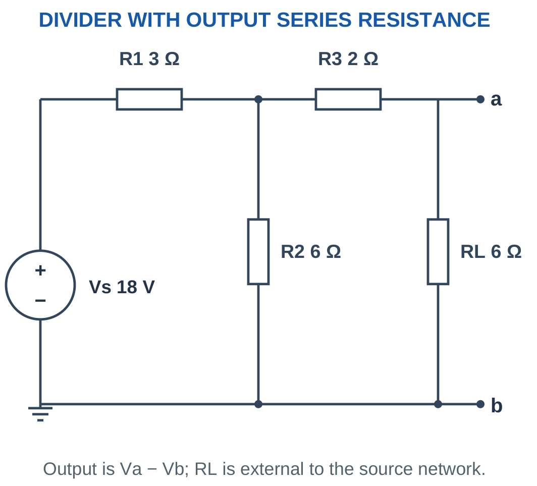
Problem: Vs = 18 V, R1 = 3 Ω, R2 = 6 Ω, R3 = 2 Ω and RL = 6 Ω.
Vth = 18 × 6/9.
Vth = 12 V.
Rth = 2 + (3 || 6).
Rth = 4 Ω.
IL = 12/(4 + 6).
IL = 1.2 A.
VL = 1.2 × 6.
VL = 7.2 V.
Worked Problem 1.104: Kilohm Extended Network

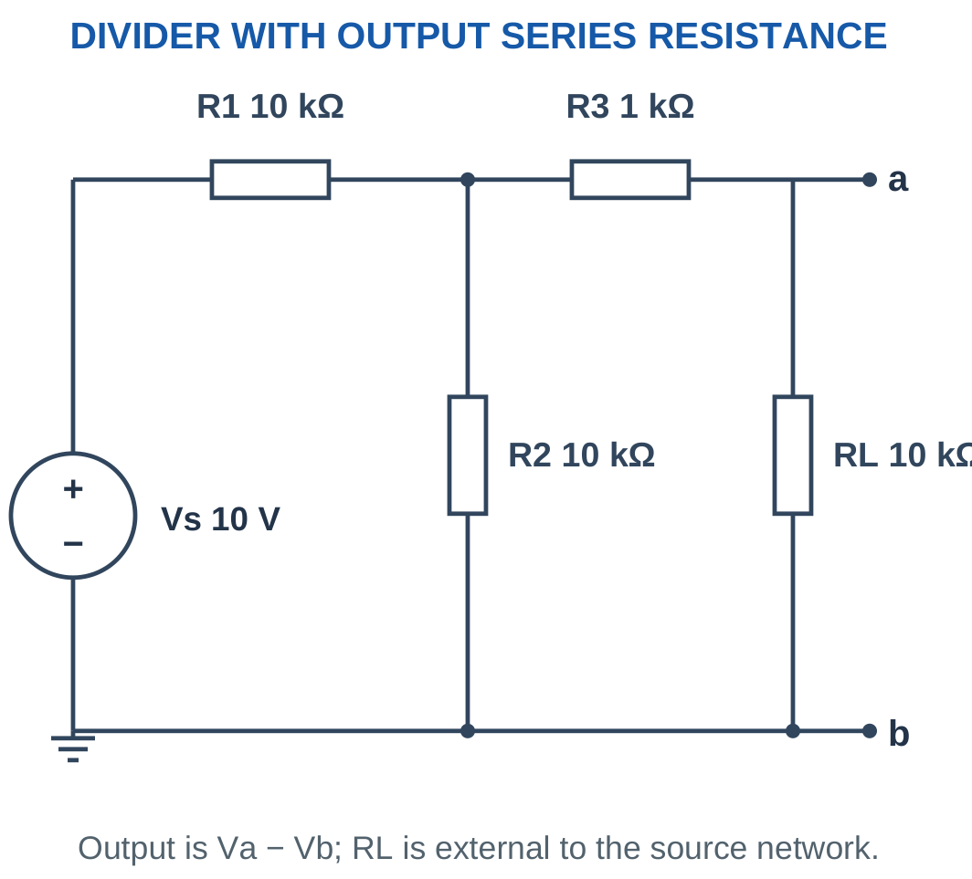
Problem: Vs = 10 V, R1 = R2 = 10 kΩ, R3 = 1 kΩ and RL = 10 kΩ.
Vth = 5 V.
Rth = 1 kΩ + 5 kΩ.
Rth = 6 kΩ.
IL = 5/(6000 + 10,000).
IL = 0.3125 mA.
VL = 0.3125 mA × 10 kΩ.
VL = 3.125 V.
Worked Problem 1.105: Several Loads on One Equivalent
Problem: Vth = 12 V and Rth = 3 Ω. Compare RL = 3 Ω, 9 Ω and 21 Ω.
For RL = 3 Ω:
IL = 12/(3 + 3) = 2 A.
VL = 6 V.
For RL = 9 Ω:
IL = 12/(3 + 9) = 1 A.
VL = 9 V.
For RL = 21 Ω:
IL = 12/(3 + 21) = 0.5 A.
VL = 10.5 V.
As load resistance increases, current falls and terminal voltage approaches the 12 V open-circuit value.
36. Ideal Meters and Basic Circuit Checking
An ideal voltmeter has infinite input resistance and is connected across the points whose voltage is measured.
An ideal ammeter has zero resistance and is inserted in series with the branch whose current is measured.
Real meters have finite input resistance or burden resistance and can change the circuit.

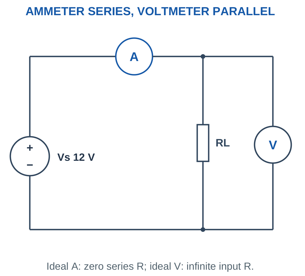
A finite voltmeter is included as a parallel load. A finite ammeter resistance is included as a series element.
Do not treat an ammeter as a voltmeter. Placing an ideal zero-resistance ammeter across a source creates a short-circuit model.
Resistance measurement in these examples refers to a de-energised isolated network. Other connected parallel paths can cause the measured equivalent resistance to differ from one component’s marked resistance.
Diagnostic Order
Check the reference node, source polarity and measurement terminals before repeating arithmetic.
A correctly solved set of equations can still answer the wrong voltage if the requested terminal pair was misidentified.
Voltage and Current Measurements

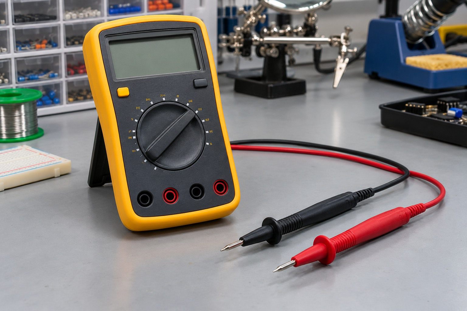
Voltage is measured between points, while current belongs to a branch. Instrument mode, range and connections must correspond to the desired quantity.
Input loading and lead placement can alter the observed result when those effects are part of the model.
Worked Problem 1.106: Finite Voltmeter Loading
Problem: Vs = 12 V, R1 = 2000 Ω and R2 = 1000 Ω. A 1 MΩ voltmeter measures across R2.
Ideal unloaded output:
V0 = 12 × 1000/3000.
V0 = 4 V.
Meter-loaded lower resistance:
Rlower = 1000 || 1,000,000.
Rlower ≈ 999.001 Ω.
Reading:
Vmeter = 12 × 999.001/(2000 + 999.001).
Vmeter ≈ 3.9973 V.
Percentage reduction:
(V0 − Vmeter)/V0 × 100.
Reduction ≈ 0.0666%.
Worked Problem 1.107: Ammeter Burden Resistance
Problem: A 5 V source drives 100 Ω. An ammeter adds 2 Ω in series.
Without meter:
I0 = 5/100.
I0 = 50 mA.
With meter:
Imeter = 5/(100 + 2).
Imeter ≈ 49.0196 mA.
Percentage reduction:
(50 − 49.0196)/50 × 100.
Reduction ≈ 1.9608%.
The meter changes the current it is intended to measure because its resistance becomes part of the branch.
37. Integrated Problems and Examination Strategy
Integrated problems combine several ideas: divider loading, source resistance, energy, method selection and terminal equivalence.
Begin with the circuit topology and define the requested references. Decide whether reduction, nodal analysis, mesh analysis or Thevenin’s theorem is appropriate.
If a particular method is requested, show the required equations even when a shortcut is available.

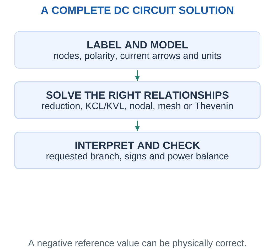
A Complete Worked-Solution Pattern
State the given data and assumptions. Identify the diagram connections. Write the governing relationship symbolically before substituting values.
Use consistent units and retain useful precision. Interpret a negative result using the assigned arrow or voltage polarity.
Verify KCL, KVL or power balance as appropriate. Report the requested current, voltage, resistance, power or energy with units.
For design questions, recompute the operating result after selecting component values. For finite instruments, include loading or burden effects before predicting the measurement.
For a Thevenin problem, preserve the source-network and load boundary throughout every stage.
Worked Problem 1.108: Design a Nominal Divider
Problem: Obtain unloaded 3 V from ideal 12 V with divider current 1 mA. Find R1 and R2, then examine a 3 kΩ load.
Total resistance:
Rtotal = 12/0.001.
Rtotal = 12 kΩ.
Lower resistor:
R2 = 3/0.001.
R2 = 3 kΩ.
Upper resistor:
R1 = 12 − 3.
R1 = 9 kΩ.
With RL = 3 kΩ:
Rlower = 3 kΩ || 3 kΩ.
Rlower = 1.5 kΩ.
Loaded output:
Vloaded = 12 × 1.5/(9 + 1.5).
Vloaded ≈ 1.7143 V.
The unloaded design meets 3 V, but the specified load substantially lowers its output.
Worked Problem 1.109: Source Power and Energy
Problem: E = 12 V, r = 1 Ω and RL = 5 Ω. The load operates for 10 minutes.
Current:
I = 12/(1 + 5).
I = 2 A.
Load power:
PL = 2² × 5.
PL = 20 W.
Internal heat rate:
Pr = 2² × 1.
Pr = 4 W.
Time:
t = 600 s.
Load energy:
WL = 20 × 600.
WL = 12,000 J.
Internal heat:
Wr = 4 × 600.
Wr = 2400 J.
The ideal EMF supplies 14,400 J, equal to these two energy transfers.
Worked Problem 1.110: Equivalent from Terminal Data
Problem: A linear network has open-circuit voltage 10 V. At a delivered current of 2 A, terminal voltage is 6 V. Find its equivalent and the current for an 8 Ω load.
Vth = 10 V.
Rth = (10 − 6)/2.
Rth = 2 Ω.
For RL = 8 Ω:
IL = 10/(2 + 8).
IL = 1 A.
VL = 1 × 8.
VL = 8 V.
The result uses the assumed linear source characteristic represented by the supplied data.
Worked Problem 1.111: Detect a Wrong Node Equation
Problem: Node A connects through 2 kΩ to +10 V and through 3 kΩ to +4 V. A student writes VA/2 + VA/3 = 0 using kΩ and mA. Correct the equation.
The other endpoints are not ground.
Correct KCL:
(VA − 10)/2 + (VA − 4)/3 = 0
Multiply by 6:
3VA − 30 + 2VA − 8 = 0.
5VA = 38.
VA = 7.6 V.
Leaving currents are:
(7.6 − 10)/2 = −1.2 mA.
(7.6 − 4)/3 = 1.2 mA.
They balance. The incorrect equation falsely treated both known source nodes as zero potential.
Worked Problem 1.112: Original Internal Power Is Not I²Rth
Problem: A 12 V divider has R1 = R2 = 6 Ω. Its external output is open. Find original source-network power and compare with the open-port Thevenin model.
Original divider current:
I = 12/(6 + 6).
I = 1 A.
Total original resistor power:
P = 1² × 12.
P = 12 W.
Equivalent parameters:
Vth = 6 V.
Rth = 3 Ω.
At the open external port:
IL = 0 A.
Equivalent resistor power:
Pth = IL²Rth.
Pth = 0 W.
Both circuits have the same open-terminal voltage and external current. Their internal power differs because Thevenin equivalence preserves terminal behaviour rather than the complete internal energy distribution.
38. Formula Sheet with Conditions
| Quantity or Method | Relationship | Main Condition |
|---|---|---|
| Constant-current charge | Q = It | Current constant over interval |
| Average current | Iavg = ΔQ/Δt | Use total charge and total time |
| Instantaneous current | i = dQ/dt | Time-varying charge description |
| Electron count | n = | Q |
| Potential difference | VAB = VA − VB | Common reference |
| Constant-voltage energy | W = VQ | Direction and sign interpreted |
| Ohmic resistor | V = IR | Constant physical conditions |
| Conductor resistance | R = ρL/A | Uniform conductor model |
| Conductance | G = 1/R | Positive finite resistor |
| Series resistance | Req = ΣRi | Same current |
| Parallel resistance | 1/Req = Σ1/Ri | Same two nodes |
| Two parallel resistors | Req = R1R2/(R1 + R2) | Two branches |
| Unloaded divider | V2 = VsR2/(R1 + R2) | No extra tap current |
| Loaded divider | Replace R2 by R2 | |
| Two-branch current divider | I1 = ItR2/(R1 + R2) | Parallel branch topology |
| General current divider | Ii = ItGi/ΣG | Common branch voltage |
| Resistor power | P = VI = I²R = V²/R | Matching element quantities |
| Passive absorbed power | p = vi | Current enters positive terminal |
| Constant-power energy | W = Pt | Power constant |
| Watt-hour conversion | 1 Wh = 3600 J | Hours converted to seconds |
| Practical delivering source | V = E − Ir | Delivery current convention |
| KCL | ΣI = 0 | Consistent current references |
| KVL | ΣV = 0 | Complete closed traversal |
| Node-to-node current | IAB = (VA − VB)/R | Actual resistor endpoints |
| Shared mesh branch | Ibranch = I1 − I2 | Directions as defined |
| Thevenin load current | IL = Vth/(Rth + RL) | Same external terminals |
| Load power | PL = IL²RL | Actual load current |
| Linear terminal relation | V = Vth − IoutRth | Delivered output-current reference |
Formula Conditions
A correct formula applied to the wrong topology gives an incorrect answer.
Divider rules depend on loading and actual node connections. Resistor power uses that resistor’s own voltage or current.
Equal wire-node potentials assume ideal conductors. Thevenin equivalence concerns the selected external terminals and does not guarantee identical internal dissipation.
Before using any expression, identify the quantity being calculated, its reference direction, its units and the assumptions behind the equation.
39. Short-Answer Questions with Complete Answers
1. Is Charge Consumed in a Resistor?
Answer: No. Charge continues through the conducting path while electrical energy is converted into heat.
In steady operation, current entering an isolated two-terminal resistor equals current leaving it. The resistor absorbs energy rather than destroying charge.
This distinction explains why the same current flows through every element in an unbranched series circuit. Charge conservation also provides the foundation for Kirchhoff’s Current Law at a junction.
2. Is EMF a Mechanical Force?
Answer: No. EMF is energy supplied per unit charge and is measured in volts.
The word force in its historical name does not make its SI unit the newton.
A practical source’s terminal voltage may fall below its EMF during delivery because current causes an internal drop. EMF describes the ideal energy-per-charge source parameter, while terminal voltage is measured across the external source terminals.
3. What Does a Negative Solved Current Mean?
Answer: It means actual conventional current flows opposite to the chosen positive arrow.
Keep the signed answer in the equations and interpret its direction afterward.
A negative current does not automatically indicate an arithmetic error or an impossible circuit. If IAB = −2 A, the actual current is 2 A from B to A. Reversing the arrow would make its numerical value positive.
4. Can Two Resistors Be in Series if Their Common Junction Has Another Branch?
Answer: Not in the ordinary series-reduction sense when the additional branch carries current.
Series reduction requires the same current through both resistors. A branching current at the junction generally makes those currents different.
Connectivity must be checked rather than judged from the way symbols are drawn. A special open branch may carry zero current under the stated condition, but that condition must be established.
5. Why Is Parallel Equivalent Resistance Smaller Than Either Branch?
Answer: Adding a positive parallel branch adds conductance.
At the same applied voltage, total current increases. Since Req = V/It, the equivalent resistance decreases.
For two positive finite branches, the result is below the smaller branch resistance. This bound is a useful numerical check. A computed parallel equivalent larger than both branches indicates an error in formula use, arithmetic or topology.
6. Why Does Loading Reduce a Divider Output?
Answer: A load across the lower resistor reduces the equivalent resistance of that lower leg.
Under a fixed ideal source, the lower leg then receives a smaller fraction of the applied voltage.
The current through the upper resistor splits between the lower resistor and the external load. Therefore the original unloaded series-divider assumption no longer applies. Replace the lower resistor with its parallel combination with the load.
7. Why Does the Current Divider Use the Opposite Resistance?
Answer: Parallel branches share voltage, so their currents vary inversely with resistance.
For two branches, algebra gives:
I1 = ItR2/(R1 + R2)
The opposite resistance appears because the smaller branch resistance must receive the larger current.
The current-divider result should be checked against this physical relationship and against the requirement that both branch currents add to total current.
8. Can an Ideal Voltage Source Absorb Power?
Answer: Yes. If current enters its positive terminal, its passive-reference power is positive.
Another source can drive energy into it in an ideal circuit model. If current leaves its positive terminal, it delivers power.
The source model alone does not determine the power sign. Current direction and terminal polarity must be considered together. This mathematical statement does not define an acceptable real-battery charging arrangement.
9. What Is the Difference Between Power and Energy?
Answer: Power is the rate of energy transfer, measured in watts.
Energy is the accumulated transfer over time and may be expressed in joules, watt-hours or kilowatt-hours.
For constant power:
W = Pt
A high-power load used briefly can transfer the same energy as a smaller load used for longer. Current, power and energy have different units and should not be substituted for one another.
10. Are Node Voltage and Resistor Voltage Always Identical?
Answer: Only when the resistor’s other terminal is at the reference node.
In general, resistor voltage is the difference between its two endpoint potentials:
Vresistor = VA − VB
Using VA/R for every resistor current falsely assumes that every other endpoint is ground.
This is a common nodal-analysis error, especially when an unknown node is connected to several known nonzero source potentials.
11. Is a Mesh Current Always a Resistor Current?
Answer: An unshared resistor may carry one mesh current directly.
A resistor shared by two meshes carries the algebraic combination of the mesh contributions. For two clockwise references, this is often I1 − I2 in the direction following mesh 1.
The branch direction must be stated. Resistor power uses the physical branch current, not one mesh variable chosen without accounting for the other mesh.
12. Are All Source-Network Currents Zero When Finding Vth?
Answer: No. Removing the external load sets only that load current to zero.
Internal resistor paths can remain complete and continue drawing current from the active sources.
An unloaded divider is a clear example: external current is zero, but its two internal resistors still form a series path across the source. Their current determines the open-circuit tap voltage.
13. Why Is an Independent Voltage Source Shorted for Rth?
Answer: Deactivation sets an ideal independent voltage source to zero volts.
Zero potential difference between its terminals is equivalent to an ideal wire.
An independent current source set to zero amperes is replaced by an open circuit instead. Separately modelled source resistance remains in the network. Dependent sources require a suitable additional method and cannot simply be removed using the independent-source rule.
14. Does Thevenin’s Theorem Reproduce Every Internal Component Power?
Answer: No. The theorem reproduces the terminal voltage-current relationship and therefore the behaviour of the external load.
Original internal branch currents and powers require the original circuit.
The equivalent resistor’s I²Rth is not a universal replacement for all original internal dissipation. An original divider may consume power even with its external output open, while its open-port Thevenin equivalent carries zero current.
15. Can an Open Branch Have Voltage and a Short Carry Current?
Answer: Yes.
An ideal open imposes zero current but can support nonzero voltage.
An ideal short imposes zero voltage but can carry a current determined by the surrounding network.
Zero current and zero voltage are different constraints. Confusing them leads to incorrect conclusions about open terminals, bypassed resistors, ideal meters and source deactivation.
40. Long-Answer Questions with Complete Model Answers
1. Explain Basic Electrical Quantities and Ohm’s Law
Answer:
Electric charge is a property of matter and is measured in coulombs. An electron carries negative elementary charge. A collection of electrons has a positive particle count but negative total signed charge.
Electric current is the rate of charge transfer through a cross-section. Average current is ΔQ/Δt, and constant-current charge transfer is Q = It.
Conventional current follows the direction positive charge would move. In metallic conductors, electron drift is opposite to conventional current.
Potential difference is defined between two points:
VAB = VA − VB
A volt corresponds to a joule per coulomb. The choice of reference node changes numerical node potentials but does not change physical potential differences.
EMF is energy supplied per unit charge by a source. It is measured in volts rather than newtons. A practical source model may include internal resistance, making loaded terminal voltage different from EMF.
Resistance relates voltage and current. For a uniform conductor, R = ρL/A. Resistivity is a material property under specified conditions, while resistance also depends on geometry.
Ohm’s law for a linear resistor under constant physical conditions is:
V = IR
Conductance is its reciprocal:
G = 1/R
When voltage is plotted vertically against current horizontally, the slope is resistance. Reversing the axes gives a slope equal to conductance.
Resistor power is:
P = VI = I²R = V²/R
The actual resistor voltage and current must be used. A negative reference current means actual current flows in the opposite direction; it does not invalidate Ohm’s law.
A complete numerical answer identifies the element, states the relevant relationship, substitutes consistent units and interprets its sign using the original references.
2. Explain Series and Parallel Reduction with Suitable Checks
Answer:
Resistors are in series when the same current must pass through each without dividing at an intermediate junction.
For series resistors, KVL gives:
V = IR1 + IR2 + …
Therefore:
Req = R1 + R2 + …
Individual drops are IRi and add to the applied voltage. A positive series equivalent exceeds each individual resistance.
Parallel resistors share the same two terminal nodes and therefore have the same voltage.
KCL gives:
It = V/R1 + V/R2 + …
Therefore:
1/Req = 1/R1 + 1/R2 + …
For two branches:
Req = R1R2/(R1 + R2)
A positive parallel equivalent is below the smallest branch resistance. Lower resistance draws more current at the common voltage.
In a mixed network, identify a genuine series or parallel group, replace it with its equivalent and redraw. Continue until the source sees a single equivalent resistance.
Then calculate source current and work backward through the reductions to recover individual branch quantities.
For R1 in series with R2 parallel to R3, first find Rp = R2 || R3. Total resistance is R1 + Rp. The parallel group receives ItRp rather than the full source voltage.
Useful checks include:
- Branch currents sum to total current.
- Complete-path voltage drops sum to source voltage.
- Series and parallel equivalent bounds are satisfied.
- Total resistor power equals ideal-source delivered power.
Visual proximity is not sufficient to establish series or parallel connections. Actual node relationships determine which reductions are valid.
3. Derive Voltage-Divider and Current-Divider Relationships
Answer:
For two unloaded series resistors across Vs, common current is:
I = Vs/(R1 + R2)
Voltage across R2 is:
V2 = IR2.
Substitution gives:
V2 = VsR2/(R1 + R2)
The resistor across which voltage is requested appears in the numerator.
The derivation assumes no additional current leaves the tap. If load RL is connected across R2, replace the lower leg with R2 || RL before applying the divider form.
For a two-branch current divider, both resistors have common voltage V.
I1 = V/R1.
I2 = V/R2.
Total current is:
It = V(1/R1 + 1/R2).
Solving for V and substituting into I1 gives:
I1 = ItR2/(R1 + R2)
Similarly:
I2 = ItR1/(R1 + R2)
The opposite resistance appears because branch current is inversely proportional to its own resistance.
For several parallel branches:
Ii = ItGi/ΣG
where Gi = 1/Ri.
Check that all branch currents add to total current. For positive resistors at a common voltage, the lower resistance receives the larger current.
Voltage division and current division are consequences of topology and Kirchhoff’s laws. They should not be applied before confirming the actual connections and loading assumptions.
4. Explain KCL, KVL and a Reliable Sign Convention
Answer:
Kirchhoff’s Current Law states that the algebraic sum of currents at a node is zero.
It follows from conservation of charge in the steady circuit model. Without net accumulation, total entering current equals total leaving current.
Assign branch arrows before writing the equation. Either take all leaving currents as positive or write entering currents on one side and leaving currents on the other.
Retain signed unknowns. A negative solution means actual current opposes its assigned arrow.
Kirchhoff’s Voltage Law states that the algebraic sum of potential changes around a closed path is zero.
For resistor traversal with its current, the potential change is −IR. Traversal against current gives +IR.
For a source, moving from negative to positive gives +E. Moving from positive to negative gives −E.
The loop may be traversed in either direction, provided every term follows that direction consistently. Reversing traversal reverses all terms and leaves the physical solution unchanged.
For a source E driving series R1 and R2:
E − IR1 − IR2 = 0.
Thus:
I = E/(R1 + R2)
KCL checks current conservation at junctions. KVL checks consistent potential differences around paths.
Power balance provides another useful check:
Σp = 0
The laws do not mean that current or voltage is consumed. Energy is transferred while charge continues through the network.
A reliable solution keeps the original references throughout the algebra and interprets signs only after the equations have been solved.
5. Describe Nodal Analysis and Its Branch-Current Logic
Answer:
Nodal analysis determines node potentials relative to one selected reference node.
Choose a convenient reference and label the other potentials. An ideal voltage source connected directly to reference may fix a node potential immediately.
At each unknown node, apply KCL. Write resistor current from a starting node to an ending node as their potential difference divided by resistance.
For A connected through R1 to V1, through R2 to V2 and through Rg to ground:
(VA − V1)/R1 + (VA − V2)/R2 + VA/Rg = 0
Grouping terms produces:
VA(1/R1 + 1/R2 + 1/Rg) = V1/R1 + V2/R2
For a positive resistor-only connection to known potentials, VA is a conductance-weighted average.
With two unknown nodes, a coupling resistor Rm contributes:
(VA − VB)/Rm
at A and:
(VB − VA)/Rm
at B.
Write one independent equation at each unknown node and solve them simultaneously.
After finding node potentials, calculate the requested branch currents using actual endpoint differences. A resistor joining two nonzero nodes does not have voltage VA alone.
Calculate powers only after the required branch voltage or current has been established.
Check signed KCL residuals and interpret negative potentials relative to the selected ground. A negative node voltage is valid and does not imply a negative resistance.
Nodal analysis is especially convenient when the number of unknown potentials is small or when current sources inject known currents directly into nodes.
6. Describe Two-Mesh Analysis and Shared-Branch Current
Answer:
For a planar resistor network, assign mesh-current variables, commonly clockwise, and apply KVL around each mesh.
An unshared resistor carries the current of its own mesh. A shared resistor receives contributions from both adjacent meshes.
For two clockwise meshes, the contributions oppose in the common branch. If downward follows mesh 1:
Ishared = I1 − I2
For outer resistors Ra and Rb, shared Rs and a left rising source E:
(Ra + Rs)I1 − RsI2 = E
−RsI1 + (Rb + Rs)I2 = 0
The diagonal coefficients contain the total resistance around each mesh. The off-diagonal coefficient is negative shared resistance for these chosen directions.
Solve the pair and convert the mesh variables into requested physical branch currents.
For a second right source with positive upper terminal, clockwise traversal crosses that source as a drop. The right-hand side of the second equation becomes −E2.
A negative mesh current reverses the corresponding reference. It does not require changing the original equation or discarding the result.
For the one-source circuit, verify:
EI1 = RaI1² + RbI2² + Rs(I1 − I2)²
The shared resistor power must use the actual difference current.
Mesh currents are a mathematical representation. They are not additional independent physical currents beyond those in the circuit branches.
A comparison with nodal analysis must therefore compare reconstructed branch quantities rather than unrelated variable names.
7. State and Apply Thevenin’s Theorem
Answer:
Thevenin’s theorem states that an eligible linear two-terminal source network can be replaced externally by an ideal voltage Vth in series with resistance Rth.
The equivalent gives the same terminal voltage and current for the external load under the model assumptions.
First identify terminals a and b and remove the external load. Keep independent sources active and calculate:
Vth = Va − Vb
under open-circuit external loading.
Next deactivate independent sources. Replace ideal voltage sources by shorts and ideal current sources by opens. Keep internal resistors and determine the resistance seen looking into a and b.
For a divider Vs, R1 and R2 viewed from the tap to reference:
Vth = VsR2/(R1 + R2)
Rth = R1 || R2
If output series resistor R3 lies between the tap and terminal a:
Rth = R3 + (R1 || R2)
while Vth remains unchanged at open circuit because R3 carries no current.
Reconnect RL:
IL = Vth/(Rth + RL)
VL = ILRL
PL = IL²RL
Verify a simple result directly in the original network.
Dependent sources cannot simply be removed using the independent-source rule. More advanced networks require a suitable test-source or other analysis.
The equivalent preserves the chosen port relationship. Original internal source currents and component powers require the original circuit.
Thevenin’s theorem is particularly useful when several different loads must be examined while the source network remains fixed.
8. Explain Power Balance and Energy Calculations
Answer:
Under the passive sign convention, absorbed power is:
p = vi
with current entering the labelled positive terminal.
Positive power indicates absorption. Negative power indicates delivery.
A positive resistor absorbs:
P = I²R
An ideal source can deliver or absorb depending on the current direction relative to its terminal polarity.
For a complete ideal DC network:
Σp = 0
Therefore total delivered power equals total absorbed power.
Include all sources and resistors in the chosen boundary. In a practical source model, ideal-EMF delivery divides between external load power and internal heating.
For constant power over a time interval:
W = Pt
Use seconds for joules and hours for watt-hours.
1 Wh = 3600 J
1 kWh = 3.6 × 10⁶ J
For variable operating states, calculate each Pi ti and add the results. An average-power calculation must use total energy divided by total elapsed time.
For example, 100 W used for two hours transfers 200 Wh or 0.2 kWh.
Under a supplied hypothetical tariff of 8 currency units per kWh, the energy charge is:
0.2 × 8 = 1.6 currency units.
Other charges are added only when specified.
Do not confuse ampere-hours with watt-hours. Ah measures charge transfer. Energy also depends on voltage.
A complete answer states the operating model, time unit, circuit boundary and interpretation of absorbed or delivered energy.
41. Final Revision and Answer Checklist
Check the Physical Meaning
Current is charge transferred per unit time. Voltage is potential difference between points. EMF is energy supplied per charge.
Resistance does not consume current. A resistor absorbs energy while the same steady charge rate enters and leaves.
Power and energy are different quantities. A watt is an energy-transfer rate, while joules and watt-hours describe accumulated energy.
Use a component’s actual voltage and current in its power calculation.
Check the Circuit Topology
Series means the same current must flow through the elements.
Parallel means both terminals are connected to the same two nodes.
A loaded divider differs from an unloaded divider because current leaves the tap.
An ideal open imposes zero current. An ideal short imposes zero voltage.
Mark nodes before combining components. The appearance of a drawing cannot replace a connectivity check.
Check the Analysis Method
KCL uses signed branch currents.
KVL uses signed potential changes around a complete loop.
Nodal currents use endpoint voltage differences.
Mesh shared-branch current uses the correct algebraic combination of mesh variables.
Thevenin sources remain active for Vth. Independent source deactivation belongs to Rth.
The external load boundary must remain unchanged throughout a Thevenin calculation.
| Final Test | What Should Agree |
|---|---|
| Units | Both sides of every equation have matching dimensions |
| KCL | Entering and leaving currents balance |
| KVL | Complete-loop potential changes sum to zero |
| Series resistance | Positive equivalent exceeds each component |
| Parallel resistance | Positive equivalent is below the smallest branch |
| Resistor power | Nonnegative for positive resistance |
| Total power | Delivered power equals absorbed power |
| Divider loading | Loaded output uses the actual parallel lower leg |
| Mesh conversion | Physical shared current includes both mesh contributions |
| Thevenin verification | Original and equivalent load results agree |
| Measurement model | Meter loading or burden is included when specified |
| Energy | Time units match the stated energy unit |
Final Memory Line
Label the circuit, write the governing equation, substitute consistent units, solve, interpret the sign and verify the result.
A numerical answer is complete when it identifies the intended terminals or branch, gives the correct unit and explains any negative reference result.