
Course: AKTU B.Tech First Year | Semester I & II
Course Codes: AAS101A–AAS101I | AAS201A–AAS201I
Streams: CSE, EE, ECE, CE, ME, BT, CH, TX & AG
Unit I Overview
Explore matter waves, wave packets, uncertainty, wavefunctions and quantised energies. The materials route connects atomic bonding and crystal structure with stress, strain and elastic response. Use the branch guide to select your prescribed topics.
Topics Covered
| Topic | Pages |
|---|---|
| Matter waves and experiments | 3–8 |
| Packets, velocities and uncertainty | 8–14 |
| Wavefunctions and wave equations | 14–18 |
| Particle in a one-dimensional box | 18–23 |
| Atomic bonding and crystal structures | 23–27 |
| Stress, strain and elastic moduli | 27–29 |
| Complete answers, formulas and revision | 30–33 |
Learning Outcomes
- Relate particle momentum to wavelength and explain the diffraction evidence.
- Distinguish phase and group velocities; apply uncertainty with its conditions.
- Interpret and normalise a wavefunction; apply the wave equations.
- Obtain allowed box states, energies and interval probabilities.
- Identify crystal packing and use the correct elastic modulus.
Included in These Notes
50 solved problems with methods and checks; 21 labelled diagrams; 10 instrument and specimen illustrations; 3 scientist sketches; complete derivations and revision answers.
Study Approach
Choose your route. Read the branch guide first. Quantum and materials topics have different branch assignments.
Read the physical model. Trace each labelled diagram and state the assumptions before using its formula.
Solve with units. Work through the examples; check normalisation, boundaries, dimensions and signs.
Revise actively. Reproduce the main derivations and use the formula sheet with its model conditions.
Coverage note: The combined PDF supports all nine streams. Not every listed topic belongs to every stream’s Unit I; the branch guide gives the exact reading route.
Stream, Course Code and Official Subject Name
| Stream | Semester I / II Codes | Official Subject Title | Unit I |
|---|---|---|---|
| CE | AAS101A / AAS201A | Physics for Sustainable Structural Systems | Full quantum unit |
| ME | AAS101B / AAS201B | Physics of Materials | Full quantum unit |
| ECE | AAS101C / AAS201C | Quantum Physics and Electronic Sensors | Full quantum unit |
| EE | AAS101D / AAS201D | Physics of Electrical Engineering Materials | Full quantum unit |
| CSE | AAS101E / AAS201E | Quantum Physics and Applications | Full quantum unit |
| BT | AAS101F / AAS201F | Physics of Materials and Biomaterials | Full quantum unit |
| CH | AAS101G / AAS201G | Physics of Process Engineering Materials | Structure and properties of materials |
| AG | AAS101H / AAS201H | Physics of Agricultural Systems and Environment | Core quantum unit |
| TX | AAS101I / AAS201I | Physics of Fibres and Textile Materials | Full quantum unit |
What Each Stream Should Read
CE, ME, ECE, EE, CSE, BT and TX: Sections 1–30 cover the complete prescribed Unit I: classical limitations, matter waves, Davisson-Germer, packets/velocities, uncertainty, wave equations, the box and probability interpretation.
AG: Prioritise Sections 2–5, 8–11 and 15–29 for wave-particle duality, matter waves, packets/velocities, the wave equations, box and wavefunction interpretation. Sections 1, 6–7 and 12–14 provide additional background; Davisson-Germer and uncertainty are not separately listed in the supplied AG Unit I.
CH: Sections 31–38 are the prescribed Unit I: atoms, bonding, BCC/FCC/HCP, lattice parameters, stress/strain and Young/bulk/shear moduli. Quantum mechanics in Sections 1–30 corresponds to CH Unit III, not CH Unit I.
Use the topic map and problem headings together. A shared document supports all streams; it does not mean every topic is prescribed in every stream’s Unit I. Semester code pairs use the same within-stream syllabus.
1. Classical Physics: Domain and Limitations
Classical mechanics describes motion using position, momentum and forces. It predicts trajectories from suitable initial conditions and remains an excellent approximation for many engineering systems. Quantum theory is more general: observable wave effects depend on wavelength, coherence and the scale of measurement, not simply on whether an object is called small.
At atomic scales, several observations resist a purely classical explanation. Classical thermal-radiation theory predicts excessive high-frequency radiation; measured black-body spectra instead fall at high frequency. The photoelectric effect shows a threshold frequency and a maximum electron energy set by frequency rather than intensity.
Classical radiating-orbit pictures do not explain stable atoms and discrete spectra. Compton scattering requires photon energy and momentum to explain the wavelength shift. Raman shifts reflect exchanges with quantised material excitations. The temperature dependence of specific heat also requires quantum ideas when classical equipartition fails.
These difficulties motivate a change of description. A quantum state predicts probabilities of outcomes and obeys a dynamical law; it is not generally a particle following one known microscopic trajectory. Conservation laws, dimensional consistency and experimental tests remain essential.
What each classical failure contributes. Black-body radiation introduces quantised energy exchange, while the photoelectric effect relates a single photon’s frequency to the available electron energy. Compton scattering tests the momentum carried by radiation. Atomic spectra and stability show that a successful matter theory must account for persistent bound structures and discrete transitions. Specific-heat departures reveal that not every microscopic mode can be treated with classical equipartition at every temperature. These examples should be connected to the appropriate observation rather than described as interchangeable proofs.
| Classical Approximation | Quantum Description |
|---|---|
| Trajectory with specified initial conditions | State and probability distributions |
| Continuous energies often possible | Bound states may have discrete energies |
| Useful at appropriate action/length scales | Required when quantum effects affect observation |
Exam answer structure. Name the observation, state the failed classical prediction, then explain the required quantum idea. Merely listing phenomena is not a full explanation.
2. Wave-Particle Duality and Quantised Exchange
Interference and diffraction reveal wave behaviour. Localised detector events and discrete energy exchange reveal particle-like aspects. These observations belong to one theory; an electron is not assumed to switch between a visible water wave and a tiny classical bead.
For a photon, E = hν and p = E/c give λ = h/p. In a one-photon photoelectric model, Kmax = hν – Φ, where Φ is the work function. The threshold is ν0 = Φ/h. Above threshold, increasing intensity mainly increases photon arrival rate; increasing frequency increases the maximum emitted-electron energy.
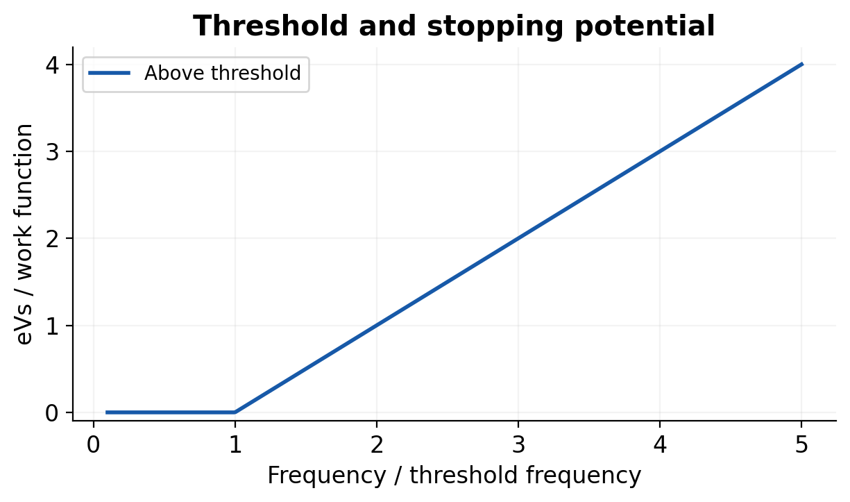
For repeated coherent single-particle experiments, individual impacts accumulate into a statistical pattern. Add probability amplitudes before taking their squared magnitude when alternatives remain coherent. Adding probabilities directly describes a different situation in which coherence is absent.
Quantum mechanics does not deny the success of classical optics or mechanics in their domains. It explains why those approximations work and where additional structure becomes measurable.
Worked Problem 1.1: Photoelectric Energy Balance
Problem: Photon energy is 3.20 eV and work function is 2.10 eV. Find maximum kinetic energy and ideal stopping potential.
Model / approach: Use the one-photon energy balance and eVs = Kmax.
Step 1: The photon exceeds the threshold, so emission is energetically allowed.
Step 2: Kmax = 3.20 – 2.10 = 1.10 eV. One electron-volt of electron energy corresponds to one volt of stopping potential.
Answer: Kmax = 1.10 eV; stopping potential = 1.10 V.
Check: A photon below 2.10 eV would not cause ideal one-photon emission even if its intensity were increased.
3. De Broglie Wavelength: Momentum Is the Starting Point
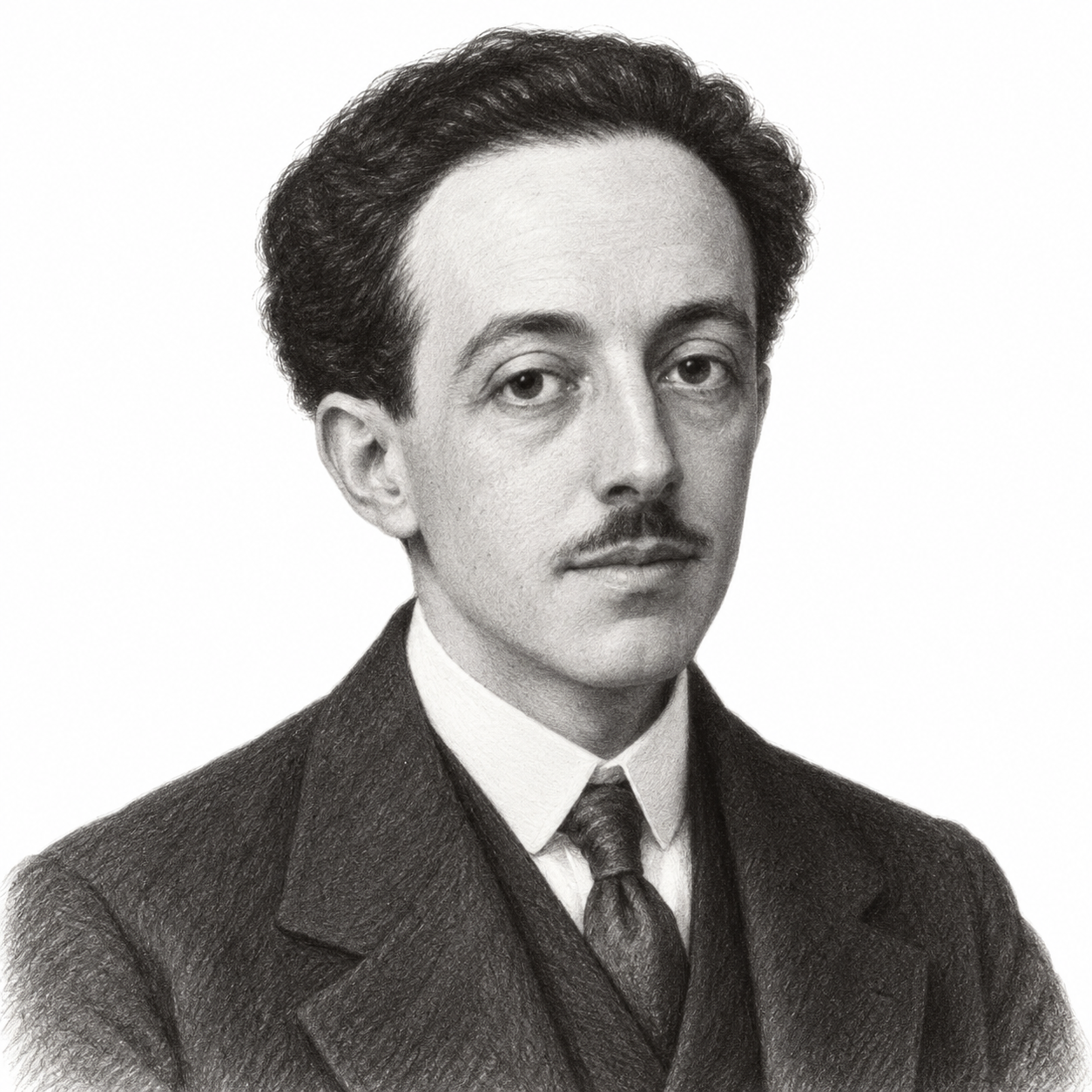
Louis de Broglie proposed in 1924 that a material particle with momentum magnitude p has an associated wavelength λ = h/p. Matter-wave interference is not restricted to charged particles: neutrons and atoms also show wave behaviour under appropriate experimental conditions.
For non-relativistic motion, p = mv. Combining this with kinetic energy K = p²/(2m) gives λ = h/(mv) = h/√(2mK). If momentum doubles, wavelength halves. If kinetic energy increases by a factor of four for the same mass, wavelength halves; the square root must not be omitted.
The matter wave describes a quantum probability amplitude. It is not necessarily an electromagnetic field oscillation and does not require a mechanical material medium. Matter-wave propagation in vacuum is possible; vacuum is essential in many electron experiments to reduce unwanted collisions.
A statement comparing heavier and lighter particles must specify what is held fixed. At equal speed, λ varies as 1/m. At equal non-relativistic kinetic energy, it varies as 1/√m. At equal momentum, the wavelengths are equal.
Derivation from kinetic energy. Begin with K = mv²/2 and p = mv. Squaring the momentum gives p² = m²v² = 2mK, so p = √(2mK) for its positive magnitude. Substitution into λ = h/p gives λ = h/√(2mK). In a ratio problem with the same mass, λ2/λ1 = √(K1/K2). At fixed K but different masses, λ2/λ1 = √(m1/m2). The quantities held fixed are part of the derivation. A mass comparison made at equal speed cannot silently use the equal-energy ratio.
Thermal convention. Using K = 3kBT/2 gives λrms-speed = h/√(3mkBT). This is a wavelength evaluated at the rms speed, not a claim that every thermal particle has one wavelength.
Worked Problem 1.2: Wavelength from Momentum
Problem: A particle has momentum magnitude 1.00 × 10^-24 kg m/s. Find its de Broglie wavelength.
Model / approach: Start with momentum rather than choosing a mass-dependent shortcut.
Step 1: λ = h/p = 6.62607015 × 10^-34 / (1.00 × 10^-24).
Step 2: Convert the resulting metres to nm by multiplying by 10^9.
Answer: λ = 6.626 × 10^-10 m = 0.6626 nm.
Check: The answer is independent of mass when the same momentum is supplied. The units J s divided by kg m/s reduce to metres.
Worked Problem 1.3: Thermal Neutron at RMS Speed
Problem: For neutrons at 300 K use the rms-speed convention v = √(3kBT/mn). Find that speed and its associated wavelength.
Model / approach: Apply the stated thermal convention; this is not one wavelength for the entire distribution.
Step 1: vrms = √[3(1.380649 × 10^-23)(300)/(1.67493 × 10^-27)].
Step 2: Use λ = h/(mn vrms); equivalently λ = h/√(3mn kBT).
Answer: vrms ≈ 2724 m/s; λ ≈ 0.1452 nm.
Check: Mean speed, most probable speed and rms speed are different. A different stated convention would produce a different characteristic wavelength.
4. Accelerating Potential and Useful Wavelength Forms
If a particle starts with negligible kinetic energy and gains energy through a potential difference of magnitude V, then K = |q|V when the field does positive work. The non-relativistic wavelength is λ = h/√(2m|q|V). An alpha particle has charge magnitude 2e; using e instead produces the wrong result.
For an electron, λ ≈ 1.2264/√V nm, or 12.264/√V angstroms, when V is in volts and the non-relativistic approximation is valid. The numerical coefficient already contains the electron mass, elementary charge and unit conversion; do not insert energy in joules into this voltage-only shortcut.
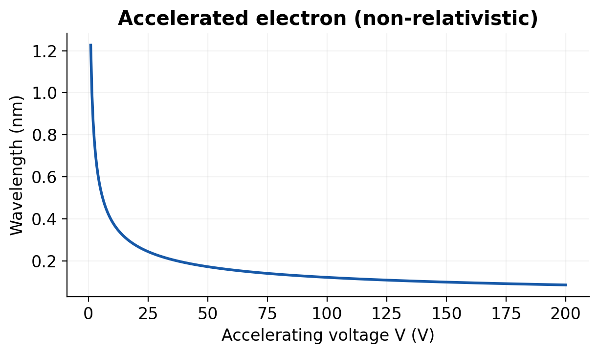
One electron-volt is the energy e times one volt: 1 eV = 1.602176634 × 10^-19 J. Also 1 nm = 10^-9 m and 1 angstrom = 10^-10 m. Write the particle and energy model before substituting numbers.
If the particle already has kinetic energy K0, add the stated energy gain before finding momentum. A potential difference by itself does not determine the final energy unless initial conditions and the sign of the work are known.

Worked Problem 1.4: Electron Accelerated Through 50 V
Problem: An electron starts with negligible kinetic energy and gains energy through 50 V. Find its non-relativistic wavelength.
Model / approach: K = eV; λ = h/√(2me eV).
Step 1: The kinetic energy gain is 50 eV = 50 × 1.602176634 × 10^-19 J.
Step 2: Substitute into the momentum expression and then λ = h/p.
Answer: λ ≈ 0.1734 nm = 1.734 angstrom.
Check: 50 eV is much smaller than the electron rest-energy scale, so the non-relativistic approximation is suitable here.
Worked Problem 1.5: Alpha-Particle Charge Factor
Problem: Use alpha mass 6.64466 × 10^-27 kg and charge +2e. It gains kinetic energy through 200 V from rest. Find λ.
Model / approach: The energy gain is 2eV, not eV.
Step 1: K = 2 × 200 eV = 400 eV.
Step 2: λ = h/√[2 ma (2e)(200 V)].
Answer: λ ≈ 7.18 × 10^-13 m = 0.00718 angstrom.
Check: The very short wavelength follows from the larger mass and the supplied energy gain. Preserve the charge magnitude in the energy relation.
Worked Problem 1.6: Electron Kinetic Energy in eV
Problem: An electron has kinetic energy 150 eV. Find λ and describe what happens if energy becomes 600 eV.
Model / approach: For the same non-relativistic mass, wavelength varies as K^(-1/2).
Step 1: Convert 150 eV to joules and evaluate h/√(2me K).
Step 2: The second energy is four times the first, so the wavelength is halved.
Answer: At 150 eV, λ ≈ 0.1001 nm; at 600 eV, ≈ 0.05007 nm.
Check: Multiplying energy by four does not divide the wavelength by four. The square-root dependence is essential.
5. Relativity and the Macroscopic Limit
The relation λ = h/p remains valid when a material particle moves relativistically. The replacements p = mv and K = mv²/2 do not. Use p = γmv, with γ = 1/√(1 – v²/c²), or pc = √[K(K + 2mc²)] when kinetic energy is supplied.
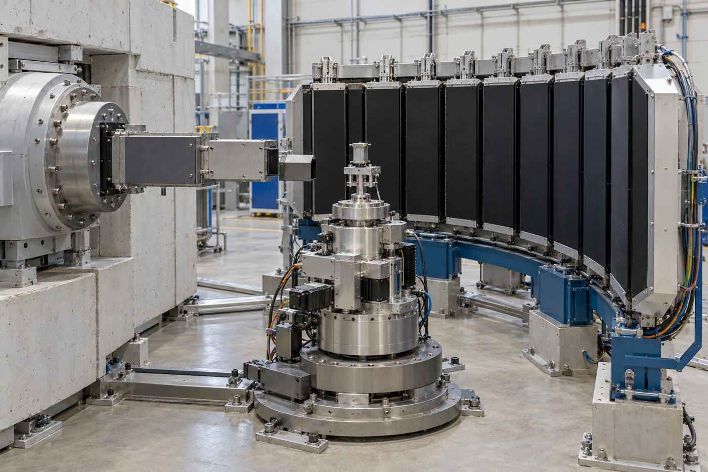
An electron accelerated through many tens of kilovolts may need a relativistic correction. A proton moving at a substantial fraction of c also needs one even if a non-relativistic formula appears algebraically simpler. The criterion is the size of v/c or K/(mc²), not the name of the particle.
A macroscopic moving object has an extremely small de Broglie wavelength under ordinary conditions. This explains why diffraction by everyday apertures is not resolved; it does not mean the wavelength formula ceases to exist. Environmental interactions and loss of coherence further suppress observable interference.
An ideal definite-momentum state at p = 0 has infinite wavelength and is spatially delocalised. A localised state contains a momentum spread. Zero average momentum is compatible with nonzero momentum uncertainty and nonzero kinetic energy.
Worked Problem 1.7: Relativistic Proton Wavelength
Problem: A proton moves at 2.00 × 10^8 m/s. Find λ using relativistic momentum.
Model / approach: Use p = γmpv because v is a substantial fraction of c.
Step 1: γ = 1/√[1 – (v/c)²].
Step 2: Find p = γmpv, then λ = h/p. Compare with h/(mpv), which would ignore relativity.
Answer: γ ≈ 1.342; λ ≈ 1.476 × 10^-15 m.
Check: The non-relativistic wavelength is larger by factor γ. A non-relativistic shortcut is not justified by simply calling the particle a proton.
Worked Problem 1.8: Macroscopic Wavelength
Problem: A 0.100 kg ball moves at 10.0 m/s. Estimate λ and compare it with a 1 mm aperture.
Model / approach: Ordinary motion is non-relativistic; p = mv.
Step 1: p = 0.100 × 10.0 = 1.00 kg m/s.
Step 2: λ = h/p; the aperture width is 10^-3 m.
Answer: λ = 6.626 × 10^-34 m; aperture/λ ≈ 1.509 × 10^30.
Check: The enormous separation of scales makes ordinary aperture diffraction unresolvable in this model. It does not remove the momentum-wavelength relation.
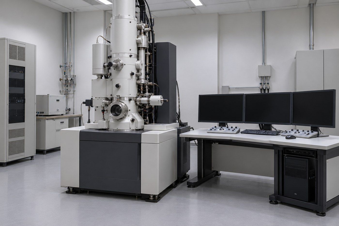
6. Davisson-Germer Experiment: Apparatus and Procedure
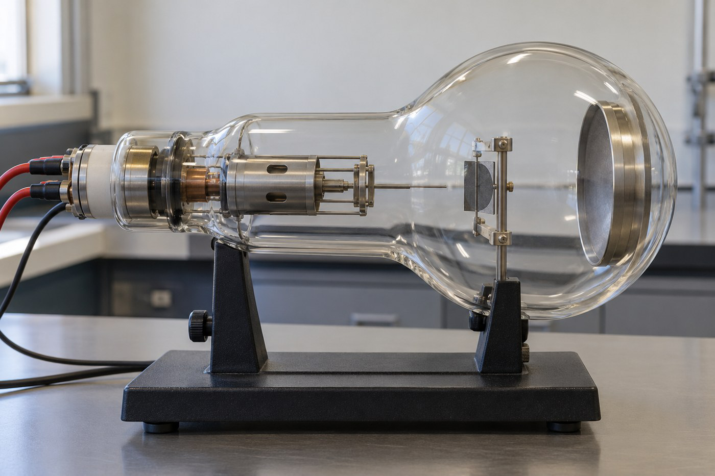
Davisson and Germer observed electron diffraction from a nickel crystal in 1927, supporting the matter-wave hypothesis. A heated filament emits electrons by thermionic emission. An accelerating potential sets their kinetic-energy scale, while apertures/focusing electrodes produce a narrow beam.
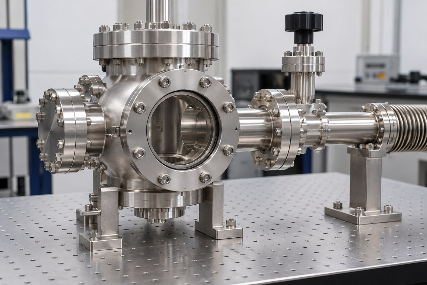
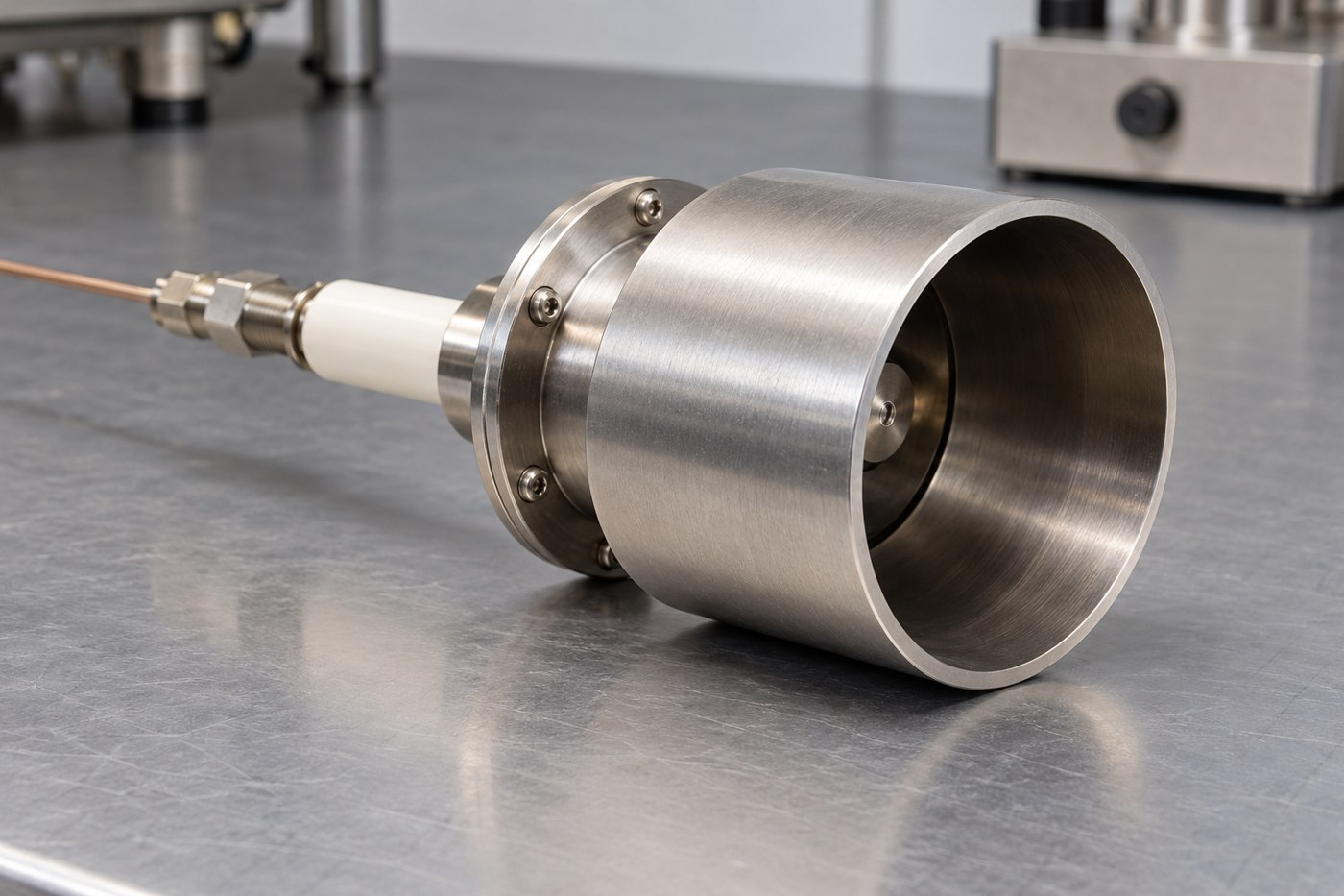
The beam strikes a nickel single-crystal target inside a vacuum chamber. A movable electron collector samples scattered electrons at different directions. A current-measuring instrument records a signal related to the collected electron intensity. The detector samples angle; it is not another accelerating electrode.
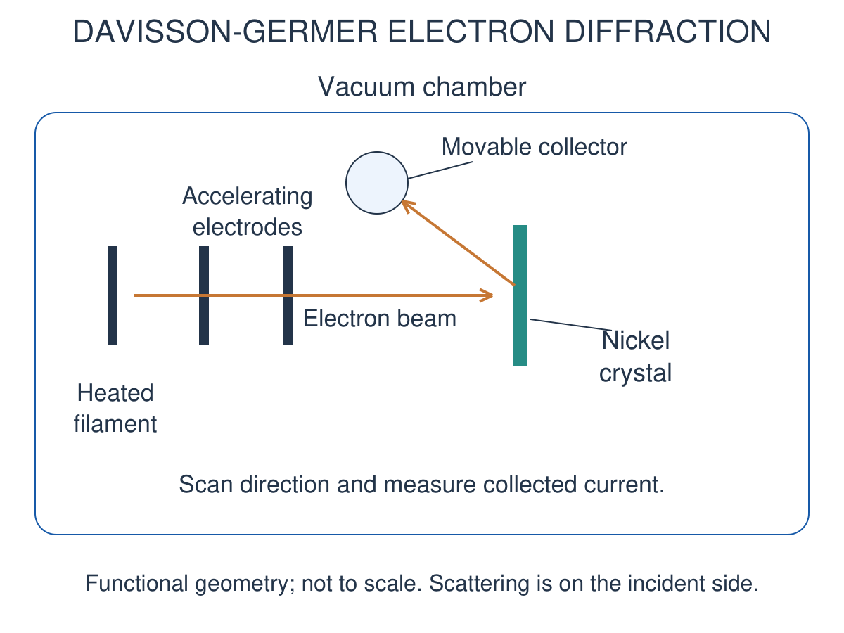
The crystal supplies an ordered scattering structure. At suitable energy and geometry, waves associated with different scattering paths interfere constructively. A peak in collected intensity at a particular angle cannot be explained by an arbitrary uniform spray of classical particles.
Procedure: Establish vacuum and beam conditions, choose an accelerating voltage, scan the collector angle and record intensity. Repeat for other voltages, identify maxima and compare the inferred wavelength with h/√(2meeV). The agreement must be quantitative, not just a claim that a peak exists.
7. Bragg Geometry and the 54 V Comparison
For waves reflected from parallel lattice planes separated by d, the path difference of the relevant rays is 2d sinθ. Constructive interference occurs when nλ = 2d sinθ. Here θ is measured from the plane, not from its normal.
The usual introductory Davisson-Germer construction reports a collector angle φ near 50° at about 54 V. With the particular convention in the accompanying geometry, 2θ + φ = 180°, giving θ = 65°. Do not substitute the collector angle directly as the Bragg glancing angle.
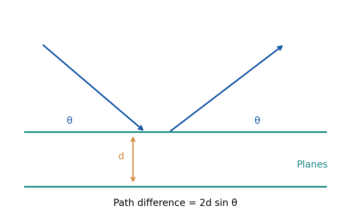
Using the supplied effective plane spacing d = 0.091 nm gives λ ≈ 0.165 nm from first-order Bragg interference. De Broglie’s non-relativistic expression at 54 V gives approximately 0.167 nm. The close agreement supports the wave interpretation. Values and geometry are part of the model; arbitrary interatomic distances cannot be substituted for d.
The observed pattern varies with electron energy and direction. A schematic peak curve illustrates this behaviour but is not a substitute for historical measured data. In an exam, identify what is controlled, what is measured and how the two wavelength estimates are obtained.
Why the extra path is twice a projection. Compare scattering from two adjacent parallel planes. The lower ray travels an additional projected segment before reflection and an equal additional projected segment after reflection. Each is d sinθ when θ is measured from the plane, giving total difference 2d sinθ. Requiring that difference to be an integer number of wavelengths produces the Bragg condition. If a diagram instead labels the angle to the normal, replace sinθ by the equivalent cosine of that complementary angle. This is geometry, not a different diffraction law.

Worked Problem 1.9: Davisson-Germer Wavelength Agreement
Problem: Use collector angle 50°, the stated relation 2θ + 50° = 180°, plane spacing 0.091 nm and voltage 54 V. Find two wavelength estimates.
Model / approach: Convert the collector angle into the Bragg glancing angle before applying nλ = 2d sinθ.
Step 1: θ = (180° – 50°)/2 = 65°. For first order λBragg = 2d sin65°.
Step 2: Independently use λdB = h/√(2me e × 54).
Answer: λBragg ≈ 0.1649 nm; λdB ≈ 0.1669 nm.
Check: The close agreement uses the supplied geometry and effective plane spacing. Substituting 50° directly as θ would not represent this construction.
Worked Problem 1.10: First-Order Bragg Angle
Problem: A wavelength 0.154 nm encounters planes separated by 0.200 nm. Find the first-order glancing angle.
Model / approach: Solve sinθ = nλ/(2d).
Step 1: For n = 1, sinθ = 0.154/(2 × 0.200) = 0.385.
Step 2: Take the inverse sine in degree mode.
Answer: θ ≈ 22.64°.
Check: The sine argument is below one, so the stated order is geometrically possible. θ is measured from the lattice plane.
8. Wave Notation, Superposition and Localisation
A sinusoidal component may be written A cos(kx – ωt + φ). The wave number is k = 2π/λ and angular frequency is ω = 2πν. k has units rad/m and ω has units rad/s; radians are dimensionless in dimensional checks.
A complex component exp[i(kx – ωt)] is a compact mathematical representation. Physical probabilities come from the appropriate squared amplitude, not from treating a complex wavefunction as an observable displacement. For a free-particle component, p = ħk and E = ħω under the stated energy convention.
Superposition combines components linearly. Two equal components reinforce where phases agree and cancel where phases differ by π. The intensity/probability density contains interference cross terms; it is not generally the sum of the separate squared amplitudes.
A single exact-k plane wave extends over all space and is not a normalisable localised state on the full infinite line. A wave packet combines a range of wave numbers to produce localisation. Greater localisation requires a broader range of components.
Worked Problem 1.11: Frequency, Wavelength and Phase Speed
Problem: A wave has frequency 5.00 × 10^14 Hz and wavelength 600 nm. Find phase speed and wave number.
Model / approach: vp = νλ and k = 2π/λ.
Step 1: Convert 600 nm to 6.00 × 10^-7 m.
Step 2: Multiply νλ and calculate 2π divided by the wavelength.
Answer: vp = 3.00 × 10^8 m/s; k ≈ 1.047 × 10^7 rad/m.
Check: Do not insert ω into νλ without the compensating 2π. Angular and ordinary frequencies are not identical numerical quantities.
9. Two-Wave Derivation of Group and Phase Velocity
Consider two waves with equal amplitude and nearby values (k1,ω1) and (k2,ω2). The identity cos a + cos b = 2 cos[(a – b)/2] cos[(a + b)/2] rewrites their sum as a slowly varying modulation multiplying a rapid carrier.
The carrier has approximately the mean k and ω. Holding its phase constant gives vp = ω/k. Holding the modulation phase constant gives the envelope speed Δω/Δk. In the narrow-band limit, vg = dω/dk.
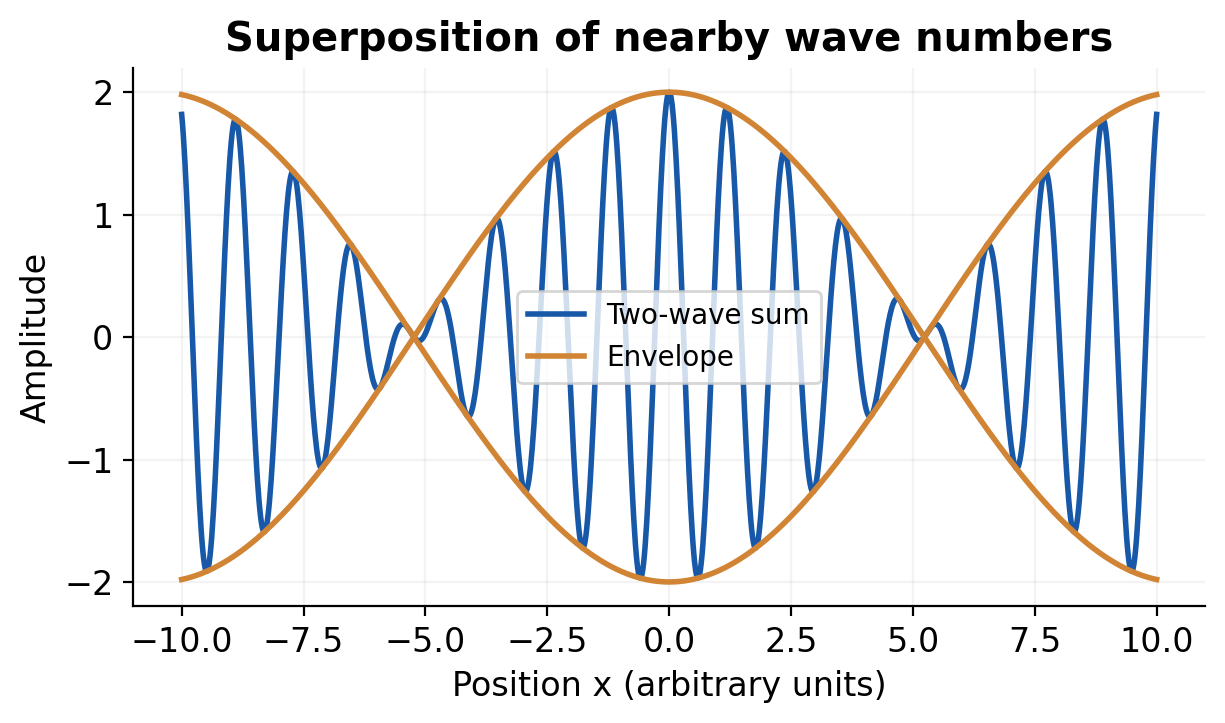
Two components alone make repeated beats rather than one isolated packet. A localised packet requires a suitable continuous or many-component spectrum. The two-wave calculation nevertheless reveals the distinction between motion of crests and motion of the envelope.
When ω(k) is linear over the relevant spectrum, all contributing group speeds agree and the ideal envelope translates without dispersive spreading. Curvature of ω(k) makes different components evolve differently. Amplitude changes or strong dispersion can require more care than the simple narrow-band picture.
Follow the two constant-phase conditions. Write the carrier factor as cos(kbar x – ωbar t) and the modulation as cos[(Δk x – Δω t)/2]. A chosen carrier crest satisfies kbar x – ωbar t = constant, so differentiating gives dx/dt = ωbar/kbar. A chosen envelope maximum satisfies Δk x – Δω t = constant, so its speed is Δω/Δk. The factor one half cancels from the second condition. Taking the limit of small separation replaces the ratio of differences by the derivative dω/dk. This also shows why substituting ω/k for both speeds misses the envelope physics.
Worked Problem 1.12: Envelope Speed from Nearby Waves
Problem: Two nearby components have f1 = 1000 Hz, f2 = 1020 Hz, k1 = 10.0 rad/m and k2 = 10.1 rad/m. Find the two-wave envelope speed.
Model / approach: Use Δω/Δk, with ω = 2πf.
Step 1: Δω = 2π × (1020 – 1000) = 40π rad/s.
Step 2: Δk = 0.1 rad/m; divide the two differences.
Answer: Envelope speed ≈ 1257 m/s.
Check: This is a general two-wave example, not a specified free-electron dispersion. Two components produce repeated beats, not one isolated packet.
10. Matter-Wave Speeds: State the Energy Convention
For a free non-relativistic Schrödinger wave with zero potential-energy reference, E = K = p²/(2m). Therefore ω = ħk²/(2m), vp = ω/k = ħk/(2m) = v/2, while vg = dω/dk = ħk/m = v.
For the relativistic total-energy convention E = γmc² and p = γmv, vp = E/p = c²/v. Differentiating E(p) gives vg = dE/dp = v, so vpvg = c² for a free massive particle under that convention.
These formulas are not contradictory. Adding a constant rest-energy term changes the phase evolution but not dE/dp. State whether the wave frequency includes rest energy before comparing phase-speed expressions.
A phase speed exceeding c does not by itself transmit information faster than light. A moving phase crest is not a material object. For the free massive-particle packet considered here, the group speed agrees with the particle speed and is below c.
| Convention | Phase / Group Result |
|---|---|
| Non-relativistic K-only, free particle | vp = v/2; vg = v |
| Relativistic total energy | vp = c²/v; vg = v |
| General narrow-band packet | vp = ω/k; vg = dω/dk |
General speed relation. Since ω = kvp(k), vg = vp + k(dvp/dk) = vp – λ(dvp/dλ). This is a dispersion relation result; a numerical use still requires a specified vp(λ).
Worked Problem 1.13: Free-Electron Phase and Group Speeds
Problem: For a free non-relativistic electron use ω = ħk²/(2me) and k = 1.00 × 10^10 m^-1. Find vp and vg.
Model / approach: Differentiate ω(k) for group velocity; divide ω by k for phase velocity.
Step 1: vp = ħk/(2me).
Step 2: vg = ħk/me = 2vp under the kinetic-energy-only convention.
Answer: vp ≈ 5.788 × 10^5 m/s; vg ≈ 1.158 × 10^6 m/s.
Check: The particle speed agrees with vg in this free-particle model. The total-relativistic-energy convention gives a different phase speed.
Worked Problem 1.14: Total-Energy Phase Speed
Problem: A free massive particle moves at 0.600c. Use the total-relativistic-energy convention to find vp and vg.
Model / approach: vp = c²/v; vg = v.
Step 1: vp = c²/(0.600c) = 1.6667c.
Step 2: vg = 0.600c; their product is c².
Answer: vp ≈ 1.667c; vg = 0.600c.
Check: The superluminal phase speed is not a superluminal material or information speed. Do not combine this vp with the K-only Schrödinger phase convention.
11. Dispersion, Packet Width and Spreading
A dispersion relation states how ω depends on k. For a free non-relativistic particle it is quadratic. A packet therefore contains components with different phase evolution and group speeds, causing its spatial width to change with time.
A narrow Gaussian packet is a useful model because its position and momentum distributions are both Gaussian. For an initially uncorrelated minimum-uncertainty free packet, σx(t) = σx(0)√[1 + {ħt/(2mσx²(0))}²]. This is a stated special model, not a universal width law for every state.
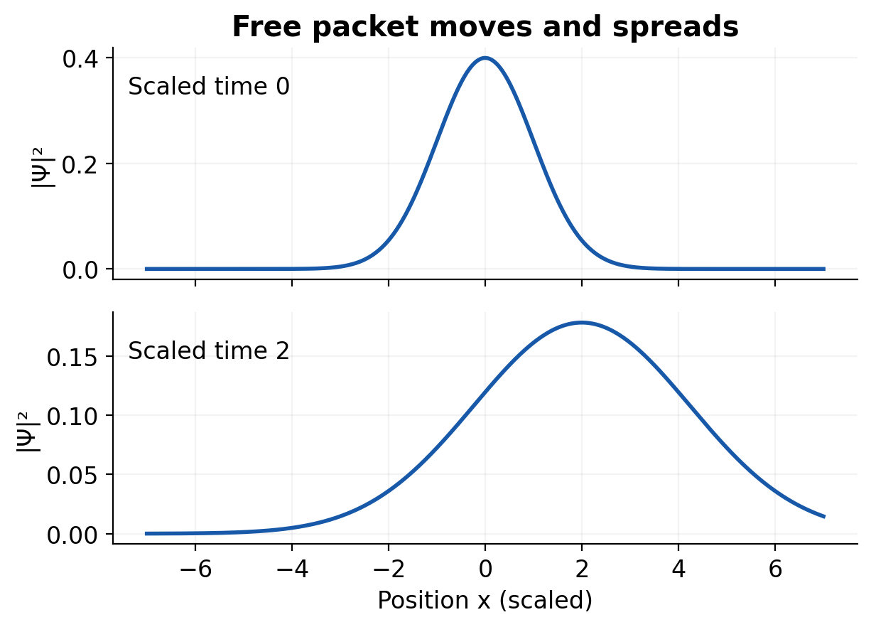
A smaller initial width gives a greater momentum spread and a shorter spreading timescale 2mσx²(0)/ħ. Increasing mass slows spreading at the same initial width. An interaction potential can alter the evolution and may support bound stationary states instead of free spreading.
Group velocity describes the motion of the central envelope for an appropriate spectrum; spreading describes a change in envelope shape. The two should not be confused. A packet can translate while simultaneously broadening.
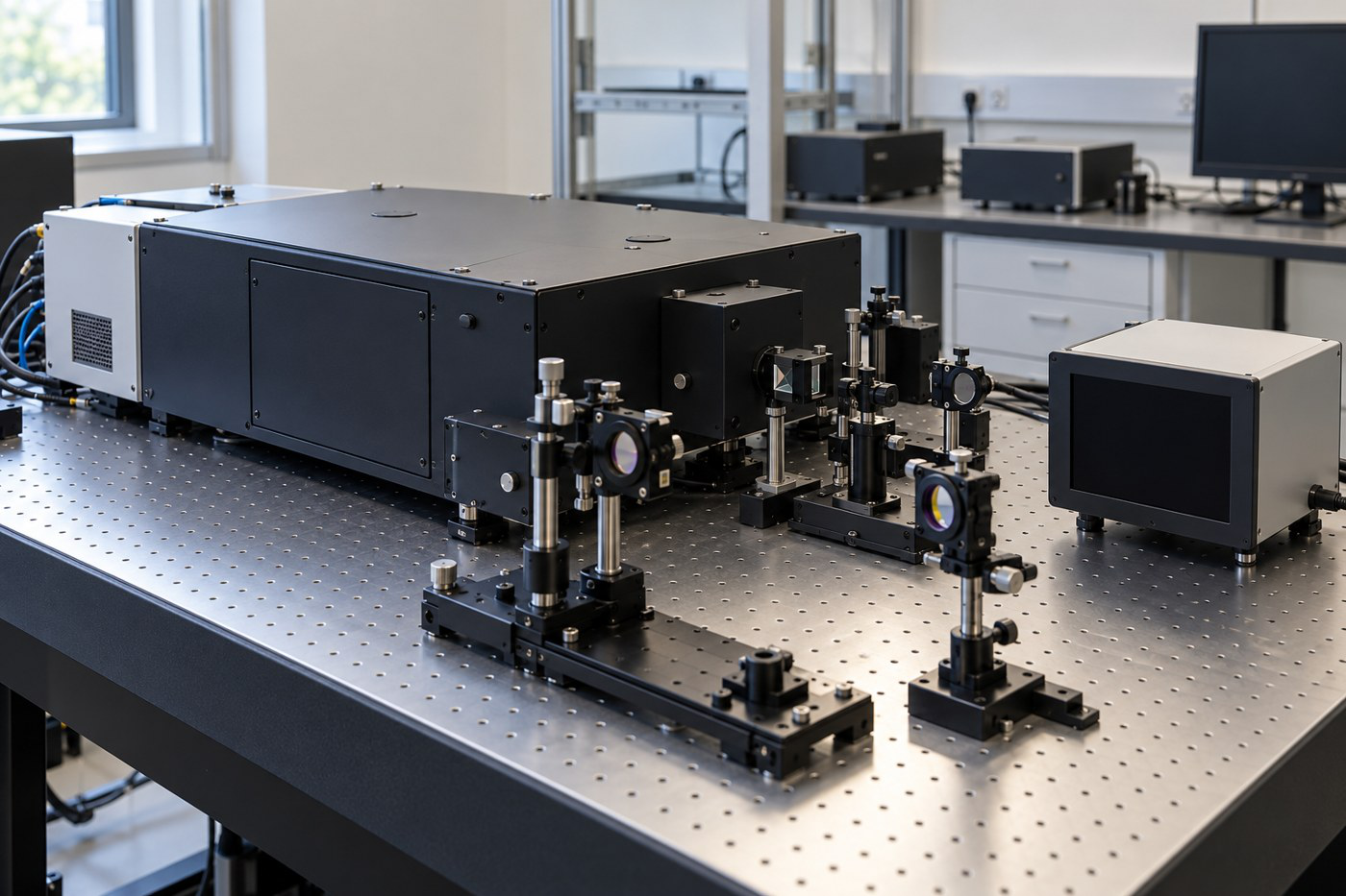
Worked Problem 1.15: Free Gaussian Spreading
Problem: An initially uncorrelated minimum-uncertainty electron packet has σx(0) = 1.00 nm. Estimate σx at 10.0 fs under the stated free Gaussian width law.
Model / approach: Use t0 = 2me σx²(0)/ħ and σx(t) = σx(0)√[1 + (t/t0)²].
Step 1: t0 is evaluated in seconds from the supplied initial width.
Step 2: 10.0 fs = 1.00 × 10^-14 s; substitute this t/t0 into the square root.
Answer: t0 ≈ 17.28 fs; σx(t) ≈ 1.155 nm.
Check: The width grows rather than translating alone. This law applies to the specifically stated initial Gaussian model.
12. Heisenberg Uncertainty: Precise Meaning and Origin
For a normalised state, σx is the standard deviation of position and σp the standard deviation of the corresponding momentum component. The precise relation is σxσp ≥ ħ/2 = h/(4π). Standard deviations describe distributions of outcomes for identically prepared states.
The relation is not merely poor instrument resolution and is not a ban on calculating an average position or average momentum. It constrains the spreads that a quantum state can possess simultaneously. A claim of equality needs a suitable minimum-uncertainty state.
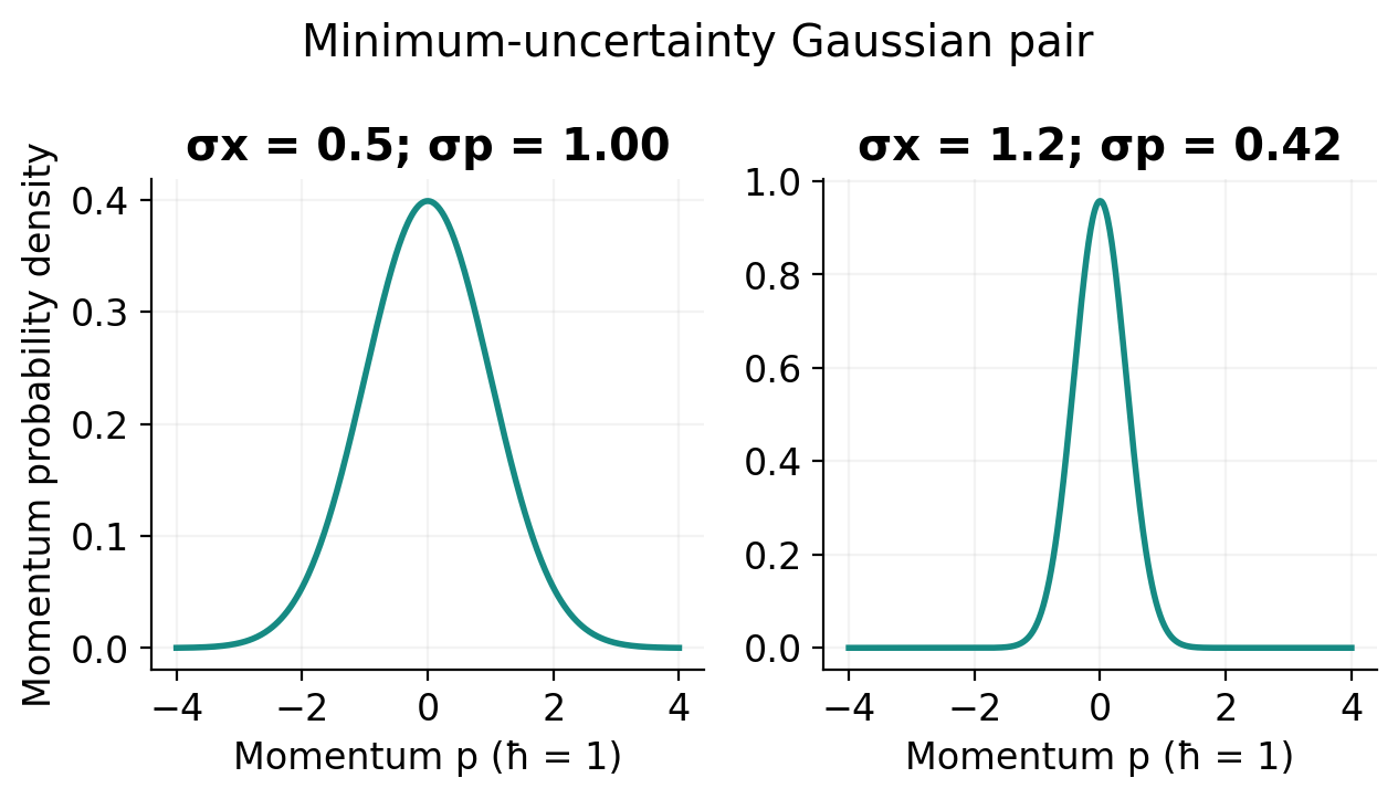
Fourier localisation gives σxσk ≥ 1/2. Since p = ħk, multiplication by ħ gives the position-momentum relation. Narrowing the spatial envelope requires a larger spread of wave numbers, providing its wave-based interpretation.
In operator form, [x,p] = iħ. Applying the Cauchy-Schwarz inequality to the deviation states (x – ⟨x⟩)ψ and (p – ⟨p⟩)ψ yields the bound from their nonzero commutator. This explains why changing experimental technology cannot remove the intrinsic limit.
What equality and component labels mean. The uncertainty relation uses the position and momentum component along the same direction. σx constrains σpx, not automatically every unrelated component. A Gaussian with the appropriate phase structure can attain equality, whereas a generic state need not. If position and momentum are correlated during free spreading, their product can increase above the initial lower limit even when the momentum distribution is unchanged. The inequality supplies a lower bound; it does not uniquely determine a complete state or every moment from one supplied width.
Proof outline with variances. Put f = (x – ⟨x⟩)ψ and g = (p̂ – ⟨p⟩)ψ. Their squared norms are σx² and σp². Cauchy-Schwarz gives σx²σp² ≥ |⟨f|g⟩|² ≥ [Im⟨f|g⟩]². The commutator [x,p̂] = iħ makes Im⟨f|g⟩ = ħ/2, yielding σxσp ≥ ħ/2. Appropriate boundary terms must vanish.
Worked Problem 1.16: Position Spread to Momentum Spread
Problem: An electron state has σx = 0.100 nm. Find the minimum σp and the corresponding non-relativistic σv bound.
Model / approach: Use σxσp ≥ ħ/2; σv = σp/me in this model.
Step 1: σp,min = ħ/(2 × 1.00 × 10^-10 m).
Step 2: Divide the resulting momentum spread by electron mass for the velocity spread.
Answer: σp ≥ 5.273 × 10^-25 kg m/s; σv ≥ 5.788 × 10^5 m/s.
Check: These are distribution spreads, not an electron’s definite momentum or speed. Equality requires an appropriate minimum-uncertainty state.
13. Uncertainty Applications: Atoms and Nuclear Localisation
Given a position spread, σp ≥ ħ/(2σx). In a non-relativistic model σv = σp/m. If an accuracy percentage is supplied, explicitly interpret it as the standard-deviation estimate used by the exercise; a generic error bar is not automatically a standard deviation.
Localisation has an energy cost. For zero mean momentum, ⟨K⟩ = σp²/(2m) in the non-relativistic model, so ⟨K⟩ ≥ ħ²/(8mσx²). This is a lower bound for a stated spread, not the exact energy of every confined state.
Atomic stability can be understood qualitatively by balancing localisation-related kinetic energy against attractive potential energy. Shrinking an electron distribution without limit drives its kinetic-energy scale upward. The argument explains a characteristic finite size; it is not a complete derivation of an atomic spectrum.
Nuclear-length localisation makes the electron momentum scale very large. Check p/(mc) before using p²/(2m); a relativistic estimate is normally required at such scales. This shows why a pre-existing, low-energy electron confined as a nuclear constituent is not a suitable model. It does not deny that electrons are produced in beta decay.
Zero mean is not zero spread. A bound electron may have ⟨p⟩ = 0 while ⟨p²⟩ is positive. Saying it can never have zero average momentum is incorrect.
Worked Problem 1.17: Percentage Momentum Uncertainty
Problem: Momentum magnitude is quoted as 5.00 × 10^-24 kg m/s with a 2.00% spread. Interpret that percentage as σp/p for this exercise and find the lower bound on σx.
Model / approach: Convert the percentage into an absolute spread before applying the uncertainty bound.
Step 1: σp = 0.0200 × 5.00 × 10^-24 = 1.00 × 10^-25 kg m/s.
Step 2: σx,min = ħ/(2σp).
Answer: σx ≥ 5.273 × 10^-10 m = 0.5273 nm.
Check: A percentage is not itself a momentum. In experimental reporting, the meaning of an error specification must be established before treating it as a standard deviation.
Worked Problem 1.18: Nuclear-Length Localisation Scale
Problem: Use an electron localisation spread σx = 1.00 × 10^-14 m. Estimate the minimum momentum scale and its relativistic kinetic-energy scale.
Model / approach: First find pscale = ħ/(2σx), then Kscale = √[(pc)² + (mec²)²] – mec².
Step 1: pscale = ħ/(2 × 10^-14 m).
Step 2: Check pscale/(me c), then evaluate the relativistic expression rather than p²/(2me).
Answer: pscale ≈ 5.273 × 10^-21 kg m/s; pscale/(me c) ≈ 19.31; Kscale ≈ 9.369 MeV.
Check: The momentum bound motivates a characteristic energy-scale estimate, not a full calculation of ⟨K⟩ for an arbitrary relativistic wave packet.
14. Energy-Time Relations and Spectral Broadening
Energy-time uncertainty requires an identified physical timescale. Time is normally a parameter in the elementary Schrödinger equation, so this relation must not be treated as the same position-momentum measurement rule with names exchanged.
A finite-duration excitation or decaying state has a frequency/energy spread. A short lifetime is associated with a broad natural spectral line; a long lifetime gives a narrower natural contribution. Other processes, such as collisions or motion, can also broaden lines.
If a problem explicitly supplies σEτ ≥ ħ/2 as its model, use σE ≥ ħ/(2τ) and σν = σE/h. Linewidth conventions matter: a Lorentzian full width at half maximum is not automatically this standard-deviation parameter. State the relation the question assumes.
Energy-time uncertainty is not permission to violate energy conservation for a short time. It relates the evolution or duration of a state/process to an energy scale under the relevant formulation. A numerical answer without a defined τ is incomplete.
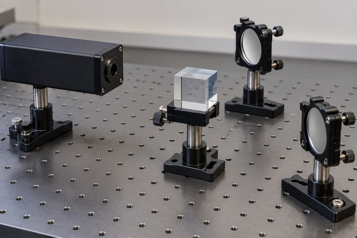
Worked Problem 1.19: Supplied Lifetime-Energy Spread Model
Problem: A problem specifies σE τ ≥ ħ/2 with τ = 10.0 ns. Find the minimum energy spread in eV and corresponding σν.
Model / approach: Use the explicitly supplied spread convention.
Step 1: σE,min = ħ/(2τ), with τ = 1.00 × 10^-8 s.
Step 2: Convert joules to eV; divide σE by h to obtain σν.
Answer: σE ≥ 3.291 × 10^-8 eV; σν ≥ 7.958 MHz.
Check: Do not label this σν as a Lorentzian FWHM without a separate linewidth convention. The relation does not authorise energy non-conservation.
15. Wavefunction and Born Probability Interpretation
The wavefunction Ψ(x,t) is a complex probability amplitude. For a single particle in one dimension, |Ψ|² = Ψ*Ψ is the position probability density. The probability of finding the particle between a and b is the integral of |Ψ|² over that interval.
For a normalised state, the integral over the entire permitted domain equals one. A density is not a probability at an exact point; for a continuous distribution, a small interval dx has probability approximately |Ψ|²dx. A density may exceed one numerically because it carries units.
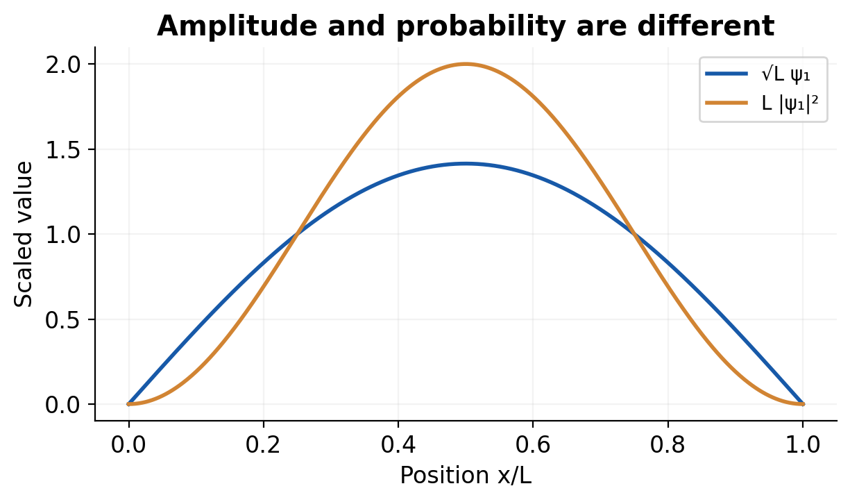
In one dimension, |Ψ|² has units m^-1, so Ψ has units m^(-1/2). In three dimensions the corresponding units are m^-3 and m^(-3/2). Dimensions prevent confusion between an amplitude and a probability.
An overall constant phase does not change |Ψ|². Relative phases between components can change interference and therefore measurable probabilities. Multiplying a state by an arbitrary real scale requires re-normalisation unless the magnitude of that scale is one.
Worked Problem 1.20: Uniform Interval Probability
Problem: A particle has uniform position density 1/L on 0 < x < L. Find the probability in L/4 < x < L/2.
Model / approach: Probability equals density integrated over interval length.
Step 1: Interval length = L/2 – L/4 = L/4.
Step 2: P = (1/L)(L/4).
Answer: P = 1/4 = 0.25.
Check: This uniform state is a supplied probability model; it is not the ground-state density of an infinite well.
Worked Problem 1.21: Density Is Not a Dimensionless Probability
Problem: A normalised one-dimensional state has |ψ|² = 4.0 × 10^8 m^-1 over a short interval of width 0.10 nm. Estimate the interval probability.
Model / approach: Use P ≈ density × interval width when the density is nearly constant there.
Step 1: 0.10 nm = 1.0 × 10^-10 m.
Step 2: P ≈ 4.0 × 10^8 × 1.0 × 10^-10.
Answer: P ≈ 0.040, or 4.0%.
Check: The density can be numerically much larger than one because it carries inverse-length units. The interval probability remains dimensionless and below one.
16. Admissible States and Boundary Behaviour
A physically admissible bound-state wavefunction must be single-valued, finite where the model requires it and square-integrable over the domain. It must satisfy the differential equation, boundary conditions and an appropriate normalisation. These conditions are tested together.
At an ordinary finite potential step with constant mass, ψ and its first spatial derivative are continuous. Discontinuous ψ generally produces an inadmissible singular kinetic term. Singular potentials have their own matching conditions; do not extend the finite-step rule to every idealised potential.
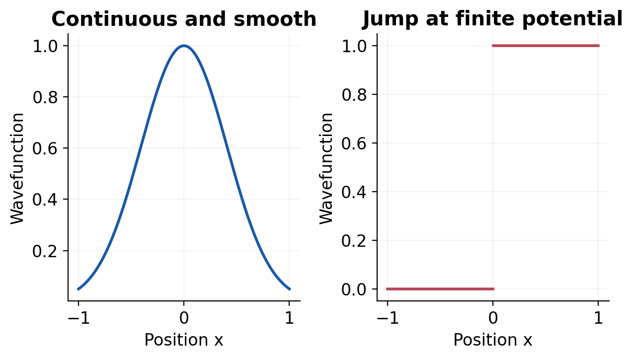
At an impenetrable wall, the wavefunction vanishes at the boundary and outside the allowed region. Its derivative need not match an exterior zero derivative across an infinite step. Confusing infinite and finite walls can eliminate valid solutions.
A plane wave on an infinite line is not square-integrable in the ordinary bound-state sense. It can still be used as an ideal scattering component with an appropriate normalisation convention. A localised packet or finite normalisation box avoids that elementary divergence.
17. Normalisation and Calculating Interval Probabilities
To normalise ψ = Af(x), calculate I = ∫|f(x)|²dx over the stated domain. Then |A|²I = 1, so a convenient positive real choice is A = 1/√I. An arbitrary overall phase remains physically irrelevant.
Never normalise over a region in which the state is defined to be zero unless that is the complete allowed domain. For piecewise states, sum the integrals over all pieces. Use the complex conjugate when the function is complex.
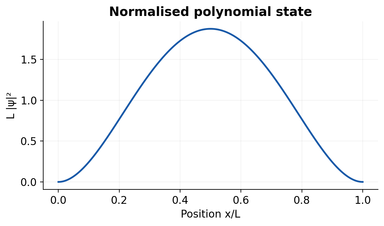
Once A is fixed, compute an interval probability from the same normalised density. The result must lie between zero and one; probabilities over disjoint exhaustive intervals sum to one. Negative values indicate an algebra or definition error.
Useful integrals include ∫x²dx = x³/3 and sin²u = (1 – cos2u)/2. A substitution y = x/L often makes the integral dimensionless and reduces unit mistakes. Normalisation fixes total probability, not the energy or momentum distribution by itself.
A practical normalisation checklist. First write the support, including any separate pieces where the function is zero. Second form ψ*ψ; only then expand algebraic or trigonometric factors. Third carry the integral with units until A is isolated. Fourth choose a convenient phase and check the total integral again. Finally calculate any requested interval probability using this same A. A common mistake is to find a new A for the subinterval, which would change the state instead of measuring its original probability. Symmetry can simplify an integral but must not discard an occupied part of the domain.
Worked Problem 1.22: Normalise a Linear Amplitude
Problem: ψ(x) = Ax for 0 < x < L and zero elsewhere, with L = 2.00 nm. Find a positive real A and probability in the right half.
Model / approach: Normalise the squared amplitude, not the amplitude.
Step 1: 1 = A²∫ from 0 to L x² dx = A²L³/3, giving A = √(3/L³).
Step 2: P(L/2,L) = A²[L³ – (L/2)³]/3 = 1 – 1/8.
Answer: A ≈ 1.936 × 10^13 m^(-3/2); right-half probability = 7/8 = 0.875.
Check: A has units m^(-3/2) because Ax must have amplitude units m^(-1/2). The larger right-half probability follows from the increasing density x².
Worked Problem 1.23: Exponential State on the Full Line
Problem: ψ = A exp(-α|x|) on the entire real line, α = 1.00 × 10^9 m^-1. Find positive A and P(|x| < 1.00 nm).
Model / approach: Exploit even symmetry of |ψ|².
Step 1: 1 = 2A²∫ from 0 to infinity exp(-2αx)dx = A²/α, so A = √α.
Step 2: The central probability is 1 – exp(-2αa), with a = 1.00 nm.
Answer: A ≈ 3.162 × 10^4 m^(-1/2); P ≈ 0.8647.
Check: Use both sides of the full-line domain. Integrating only the positive side would incorrectly miss half the total probability.
18. Operators, Averages and Uncertainty Calculations
For the elementary position representation, x̂ acts by multiplication, p̂ = -iħ∂/∂x and the free kinetic-energy operator is -ħ²∂²/(2m∂x²). These operations act on a wavefunction; they are not numbers to be substituted before differentiating.
For a normalised state, ⟨x⟩ = ∫ψxψ dx and ⟨p⟩ = ∫ψ(-iħ∂ψ/∂x)dx. Similarly obtain second moments. The variance is σA² = ⟨A²⟩ – ⟨A⟩², not ⟨A²⟩ – ⟨A⟩.
An eigenstate satisfies Âψ = aψ and gives that observable value a with certainty in the ideal measurement model. It need not be an eigenstate of a different operator. A real standing-wave box state has zero average momentum but nonzero kinetic energy.
Expectation values describe averages over many identically prepared measurements, not necessarily a value seen in one trial. Check that ⟨x⟩ lies within a finite support interval and that the computed variance is nonnegative.
| Observable | Position Representation |
|---|---|
| Position | x times ψ |
| Momentum | -iħ ∂ψ/∂x |
| Kinetic energy | -ħ² ∂²ψ/(2m ∂x²) |
| Total energy operator | Hamiltonian: kinetic + potential |
Worked Problem 1.24: Momentum-Operator Eigenvalue
Problem: Apply p̂ = -iħ d/dx to ψ = A exp(ikx), with k = 2.00 × 10^10 m^-1. Identify the eigenvalue.
Model / approach: Differentiate the function before simplifying the operator expression.
Step 1: dψ/dx = ikψ.
Step 2: p̂ψ = -iħ(ikψ) = ħkψ.
Answer: Momentum eigenvalue p = ħk ≈ 2.109 × 10^-24 kg m/s.
Check: The opposite spatial phase exp(-ikx) has eigenvalue -ħk. An infinite-line plane wave uses an ideal scattering normalisation, not ordinary bound-state normalisation.
Worked Problem 1.25: Variance from Two Moments
Problem: A state has ⟨x⟩ = 2.00 nm and ⟨x²⟩ = 5.00 nm². Find σx.
Model / approach: Variance is second moment minus the square of the first moment.
Step 1: σx² = 5.00 – (2.00)² = 1.00 nm².
Step 2: Take the positive square root.
Answer: σx = 1.00 nm.
Check: Subtracting ⟨x⟩ without squaring it would mix incompatible units. A negative variance would signal inconsistent data or an algebra error.
19. Time-Dependent Schrödinger Equation
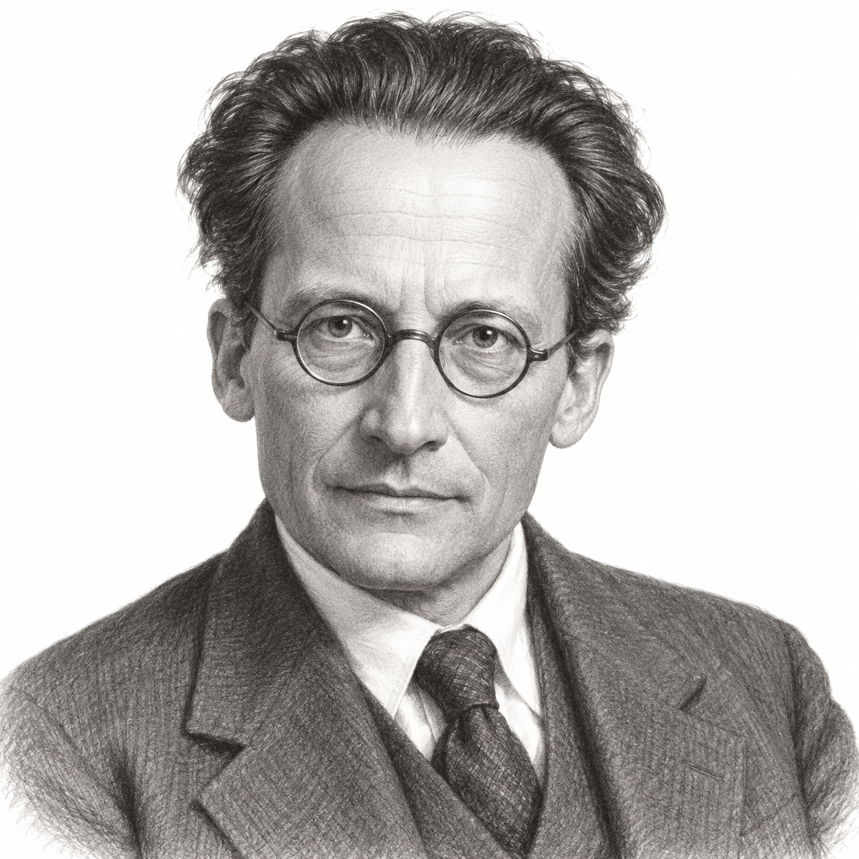
The time-dependent Schrödinger equation is the dynamical postulate for the non-relativistic state considered here. For one particle in one dimension:
iħ∂Ψ/∂t = [-ħ²/(2m) ∂²/∂x² + U(x,t)]Ψ.
One motivation comes from a free component Ψ = A exp[i(kx – ωt)]. Differentiation gives iħ∂Ψ/∂t = ħωΨ and -ħ²∂²Ψ/(2m∂x²) = ħ²k²Ψ/(2m). With E = ħω and p = ħk, the free-particle relation E = p²/(2m) is reproduced.
This motivation does not derive quantum mechanics solely from classical mechanics. Promoting energy and momentum to operators introduces new physics. The equation is first order in time and second order in position; specify an initial state plus the appropriate spatial conditions.
The potential-energy term has units of energy and multiplies the state. Do not replace it by electric voltage without the appropriate charge factor. A solution must satisfy the equation over the domain, not just at one chosen point.
20. Separation of Variables and the Stationary Equation
When U depends on x but not time, try Ψ(x,t) = ψ(x)T(t). Substitute into the time-dependent equation and divide by ψT where appropriate. The time-dependent side equals a spatial expression, so both equal a separation constant E.
The time equation is iħ dT/dt = ET, giving T(t) = exp(-iEt/ħ) apart from a constant. The spatial equation becomes -ħ² d²ψ/(2m dx²) + U(x)ψ = Eψ. This is the time-independent Schrödinger equation (TISE).
Equivalently, d²ψ/dx² + [2m(E – U)/ħ²]ψ = 0. For a constant potential and E greater than U, the elementary spatial solutions are oscillatory. If E is below a finite constant barrier, exponential behaviour is possible; this does not imply a negative probability.
Allowed energies follow from the equation together with boundary and normalisation conditions. The TISE alone does not say every potential has a discrete spectrum. Free/scattering and bound-state boundary conditions can give different spectral structures.
Separation step by step. After substitution, iħψ(dT/dt) = T[-ħ²ψ″/(2m) + Uψ]. Division gives iħ(T′/T) = -ħ²(ψ″/ψ)/(2m) + U. The left side depends only on time; the right side depends only on position. Their common constant is E for a nontrivial separated solution. Integrating T′/T = -iE/ħ gives the exponential time factor. Multiplying the spatial expression back by ψ gives the TISE. The argument requires a time-independent potential; a general time-dependent potential does not permit this simple separation.
21. Free Components and the Meaning of Stationary State
For U = 0, a component exp(ikx) has momentum ħk and energy ħ²k²/(2m). Components with +k and -k have the same kinetic energy but opposite momenta. A standing wave combines travelling components and is not a classical particle moving only one way.
For a stationary energy eigenstate, Ψ = ψ exp(-iEt/ħ). Its probability density is |ψ|² because the time factor has unit modulus. The wavefunction has time-dependent phase even when the density does not change.
Stationary does not mean that every observable is zero or that the particle has a known fixed position. A real box eigenfunction has zero probability current in this simple model while retaining positive kinetic energy and a spatial probability distribution.
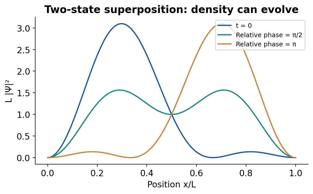
A superposition of different energies generally has time-dependent interference terms in its density. If ψ1 and ψ2 evolve with different frequencies, their relative phase changes. An incoherent mixture and a coherent superposition must not be identified merely because they share some average energies.
Worked Problem 1.26: Energy of a Free Component
Problem: For a free electron component with k = 2.00 × 10^10 m^-1, find energy and angular frequency in the non-relativistic K-only model.
Model / approach: E = ħ²k²/(2me); ω = E/ħ.
Step 1: Evaluate E in joules using the squared wave number.
Step 2: Divide by e for eV and by ħ for ω.
Answer: E ≈ 15.24 eV; ω ≈ 2.315 × 10^16 rad/s.
Check: The positive and negative k components have equal energy in this free model but opposite momentum.
Worked Problem 1.27: Phase Period of a Stationary State
Problem: A stationary state has E = 1.00 eV relative to the declared energy zero. Find the time for its phase factor exp(-iEt/ħ) to change by 2π.
Model / approach: Set ET/ħ = 2π, so T = h/E.
Step 1: Convert 1.00 eV to e joules.
Step 2: T = h/(1.00 eV).
Answer: Phase period ≈ 4.136 fs.
Check: The stationary probability density does not oscillate at this period. A global phase is not itself an observable position signal.
22. Confinement Model and Wall Conditions
An infinite one-dimensional well is an idealised confinement model: U = 0 for 0 < x < L and U is infinite outside. The state is zero outside and must vanish at x = 0 and x = L. Inside, the particle obeys the free-form TISE.
The model captures how a finite allowed length and boundary conditions produce discrete energies. It omits finite barrier penetration, interactions and detailed material band structure. Use it to understand quantisation, not as an exact model of every nanostructure.
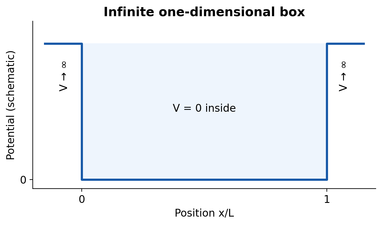
Inside the well, write ψ = A sin(kx) + B cos(kx). The left boundary gives B = 0. The right boundary requires sin(kL) = 0 for a nonzero state, so kL = nπ.
The n = 0 choice gives the zero function and cannot be normalised. Distinct physical standing-wave states may be labelled n = 1,2,3,…; negative n merely changes an overall sign of the sine state already represented.
23. Box Eigenfunctions: Complete Derivation
From kn = nπ/L, the spatial state is A sin(nπx/L). Impose normalisation:
1 = |A|²∫ from 0 to L sin²(nπx/L) dx = |A|²L/2.
Choose A = √(2/L).
Thus ψn(x) = √(2/L) sin(nπx/L) inside the well and zero outside. The amplitude has units L^(-1/2). Different n values have different numbers of oscillations but the same total integrated probability.
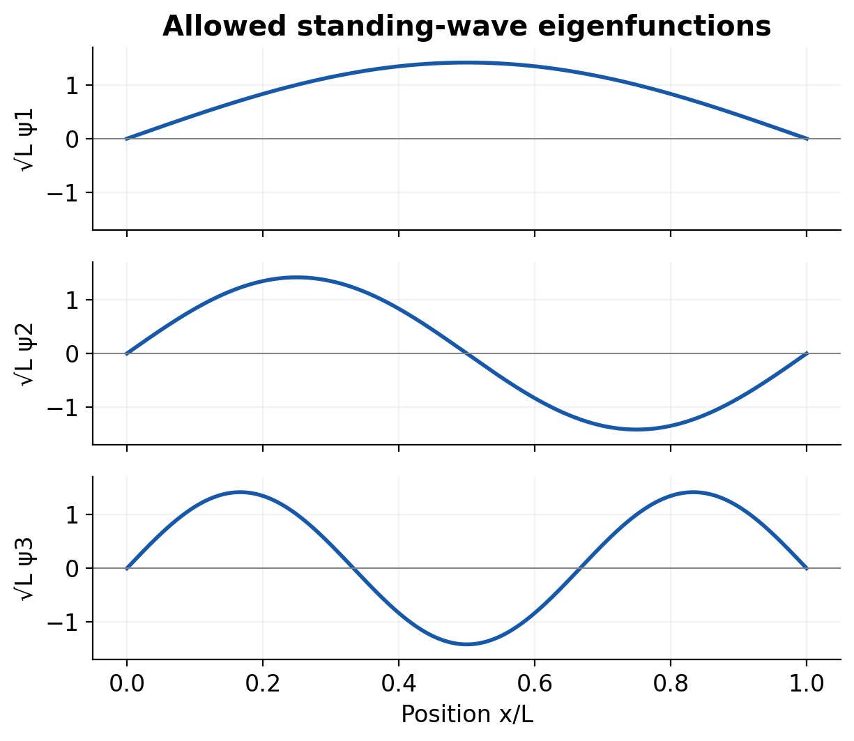
The complete stationary solution includes exp(-iEnt/ħ). This phase factor is needed when comparing coherent components, even though it disappears from one eigenstate’s density.
Each standing-wave condition can also be written L = nλn/2, giving λn = 2L/n. This wavelength is associated with the travelling components of the standing wave; it does not assign the bound particle one definite signed momentum.
Rejecting the zero solution correctly. Setting B = 0 at the left wall does not yet quantise energy. Quantisation follows when the nonzero remaining amplitude must also satisfy the right wall. The option A = 0 satisfies both walls but gives zero total probability, so it cannot describe the particle. The remaining option sin(kL) = 0 selects nπ/L. For n = 0 the sine function still vanishes everywhere. This explains both the discrete positive index and the missing zero-energy bound state without adding a separate arbitrary rule.
Worked Problem 1.28: Normalised Box Amplitude and Wave Number
Problem: For n = 3 in a box of width 1.00 nm, find the positive normalisation factor, k3 and standing-wave wavelength.
Model / approach: Use A = √(2/L), kn = nπ/L and λn = 2L/n.
Step 1: Substitute L = 1.00 × 10^-9 m.
Step 2: Calculate k3 and λ3 independently from the boundary condition.
Answer: A ≈ 4.472 × 10^4 m^(-1/2); k3 ≈ 9.425 × 10^9 m^-1; λ3 ≈ 0.6667 nm.
Check: The nth eigenfunction has n – 1 internal nodes. The standing wave does not have one definite signed travelling momentum.
24. Box Energies, Scaling and Zero-Point Energy
Using E = ħ²k²/(2m), the allowed levels are En = n²π²ħ²/(2mL²) = n²h²/(8mL²). The ground level is positive because the zero function is the only n = 0 candidate under these boundaries.
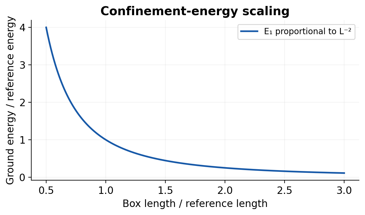
Ground-state energy varies as 1/(mL²). Halving L raises every level by a factor of four. Doubling mass halves each level for the same width. This scaling is often faster and clearer than repeating the full constant substitution.
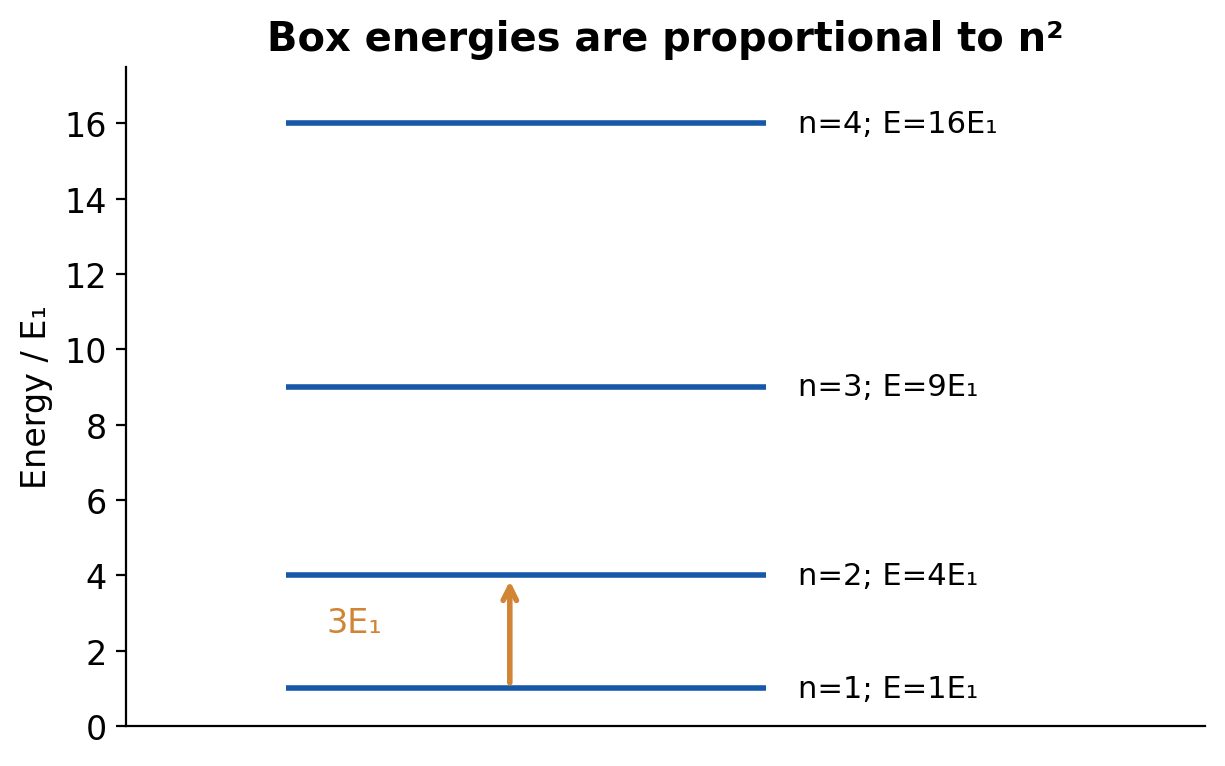
For an electron with L in nm, En ≈ 0.37603 n²/L² eV. This shortcut assumes electron mass and the infinite-well non-relativistic model. A value for a neutron or proton needs the appropriate mass.
Adjacent spacings are En+1 – En = (2n + 1)E1. They are not equal. Zero-point energy is a property of the confined ground state here, not a claim that every possible free particle has the same nonzero minimum energy.
Worked Problem 1.29: Electron Box Energy Levels
Problem: An electron occupies an infinite box of width 1.00 nm. Find E1, E2 and E3.
Model / approach: Compute E1 once; use En = n²E1.
Step 1: E1 = h²/(8meL²), with L in metres.
Step 2: Multiply E1 by 4 and 9 for n = 2 and 3.
Answer: E1 ≈ 0.376 eV; E2 ≈ 1.504 eV; E3 ≈ 3.384 eV.
Check: The ground level is not zero and the spacing is not uniform. The electron mass and impenetrable-wall model are part of the result.
Worked Problem 1.30: Width Inferred from Ground Energy
Problem: An electron infinite-well model has ground energy 1.50 eV. Find the width.
Model / approach: Rearrange E1 = h²/(8meL²) to solve for L.
Step 1: Convert the supplied ground energy to joules.
Step 2: L = h/√(8meE1).
Answer: L ≈ 0.5007 nm.
Check: The result is a width in the specified model. If the given energy were E2 instead, the inferred width would differ by a factor of two.
25. Box Probability, Nodes and Useful Symmetry
For an eigenstate, ρn(x) = (2/L)sin²(nπx/L). It is nonnegative, vanishes at the walls and integrates to one. Internal nodes occur at x = jL/n for j = 1,…,n – 1.
For a ≤ x ≤ b:
P = (b – a)/L – [sin(2nπb/L) – sin(2nπa/L)]/(2nπ).
Derive this by integrating sin² using its double-angle identity. Keep the supplied state index n when evaluating the sine terms.
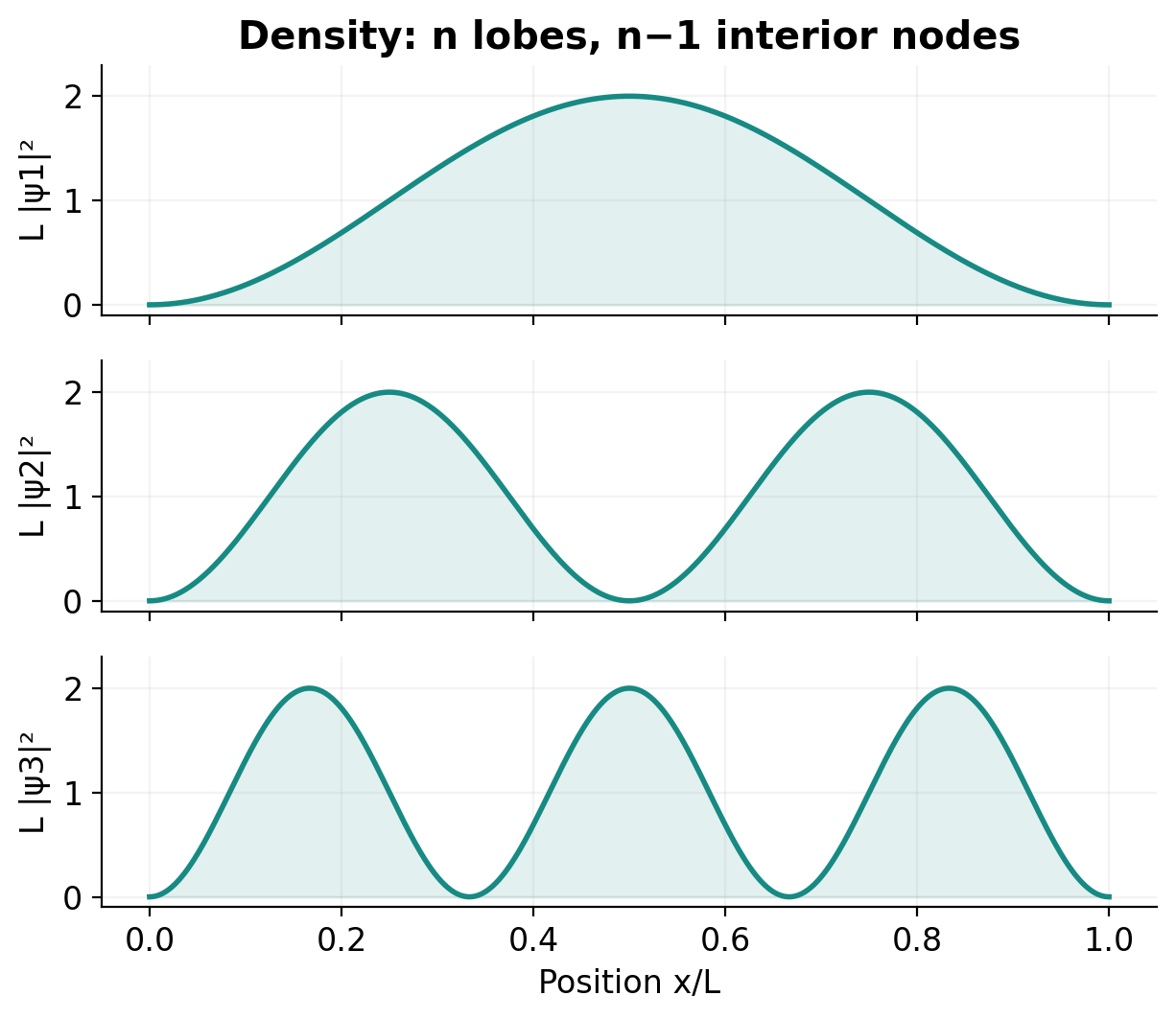
The ground-state density is largest at the centre, while the second state has a node there. A node at one exact position does not imply a finite interval around it has zero probability. Distinguish a point density from an integrated probability.
Every eigenstate’s density is symmetric about L/2, giving probability one half in each half of the box and mean position L/2. This symmetry does not make the density uniform; the central-half probability depends on n.
Integrate before interpreting the picture. Using sin²u = (1 – cos2u)/2, the density integral becomes (1/L)∫dx – (1/L)∫cos(2nπx/L)dx. The first term gives (b – a)/L. The second gives the sine difference divided by 2nπ. The first term resembles a uniform classical probability; the oscillatory correction carries the quantum-state dependence. Over the full box the correction vanishes and the first term equals one. For small intervals, use the exact limits or a controlled density-times-width approximation rather than counting visible peaks.
Worked Problem 1.31: Probability in the Central Half
Problem: Find probability in L/4 < x < 3L/4 for box states n = 1 and n = 2.
Model / approach: Integrate the normalised sin² density using the interval formula.
Step 1: For n = 1, P = 1/2 + 1/π.
Step 2: For n = 2, the sine-boundary correction vanishes, giving P = 1/2.
Answer: P1 ≈ 0.8183; P2 = 0.5000.
Check: Both states give probability 1/2 in either left or right half, yet their central-half probabilities differ. Symmetry does not imply a uniform density.
26. Energy Transitions and Width Estimation
If a system makes a permitted transition between box levels, the energy difference is ΔE = Efinal – Einitial. The magnitude sets an exchanged photon energy when a photon mediates the transition: hν = |ΔE| and λphoton = hc/|ΔE|.
The photon wavelength is not the particle’s box standing-wave wavelength 2L/n. One concerns an energy difference of radiation; the other concerns matter-wave spatial variation in the confined state. Their formulas contain different physical quantities.
The simple level-spacing calculation gives the energy required or released, but does not by itself prove every transition has a nonzero interaction matrix element. Selection rules depend on the perturbation and symmetry. State the assumption of a permitted transition in a numerical exercise.
If E1 is given, L = h/√(8mE1). If another level is given, first divide by n² or include n in the width formula. A width derived from this model is a model parameter, not an independently verified geometric measurement.
Worked Problem 1.32: Box Transition Photon
Problem: For the 1.00 nm electron box, assume a permitted transition from n = 3 to n = 2. Find emitted photon energy and wavelength.
Model / approach: The photon carries the level-energy difference.
Step 1: ΔEphoton = (9 – 4)E1 = 5E1.
Step 2: λphoton = hc/ΔEphoton after consistent energy conversion.
Answer: Photon energy ≈ 1.88 eV; λ ≈ 659.4 nm.
Check: This radiation wavelength is not the matter-wave value 2L/n. A level difference alone does not establish a selection rule for every possible interaction.
27. Box Averages and the Uncertainty Check
For a normalised box eigenstate, ⟨x⟩ = L/2 and ⟨x²⟩ = L²[1/3 – 1/(2n²π²)]. Therefore σx = L√[1/12 – 1/(2n²π²)]. These follow by integrating the normalised sin² density.
The expectation ⟨p⟩ is zero for the real standing-wave spatial state, while ⟨p²⟩ = (nπħ/L)². Hence σp = nπħ/L. A zero average momentum is entirely compatible with positive energy.
The product σxσp = ħ√[n²π²/12 – 1/2] exceeds ħ/2 for the ground state and larger n. The box ground state is not a minimum-uncertainty Gaussian. Treating the inequality as equality would give an incorrect exact box energy.
Check dimensions: σx has length units, σp momentum units and their product action units. In an exam, computing a variance requires both the first and second moments; quoting only ⟨x²⟩ is insufficient.
From moments to physical conclusions. The symmetry of sin² about L/2 gives ⟨x⟩ directly. For ⟨x²⟩, retain the x² factor while applying the double-angle identity and integration by parts; the resulting boundary contribution supplies the term -L²/(2n²π²). For momentum, differentiation of the real sine state gives a cosine and the full integral for ⟨p⟩ vanishes. Applying the second derivative returns -(nπ/L)² times the sine, so ⟨p²⟩ is positive. The kinetic energy therefore remains positive even though the first momentum moment is zero.
Worked Problem 1.33: Ground-State Box Uncertainty
Problem: For an electron in the ground state of a 1.00 nm box, compute σx, σp and their product in units of ħ.
Model / approach: Use the exact moments of the box state, not a forced equality in the uncertainty bound.
Step 1: σx = L√[1/12 – 1/(2π²)].
Step 2: σp = πħ/L; multiply the two spreads.
Answer: σx ≈ 0.1808 nm; σp ≈ 3.313 × 10^-25 kg m/s; product ≈ 0.5679 ħ.
Check: The product is greater than ħ/2. The real standing-wave state has zero ⟨p⟩ but a nonzero momentum spread.
28. Orthogonality and Coherent Superposition
Different normalised box eigenfunctions satisfy ∫ψm*ψn dx = 0 for m ≠ n and one for m = n. This orthogonality is a mathematical relation between states, not a claim that their probability densities never overlap in space.
For Ψ = c1ψ1exp(-iE1t/ħ) + c2ψ2exp(-iE2t/ħ), normalisation gives |c1|² + |c2|² = 1. Energy measurements yield E1 or E2 with these probabilities.
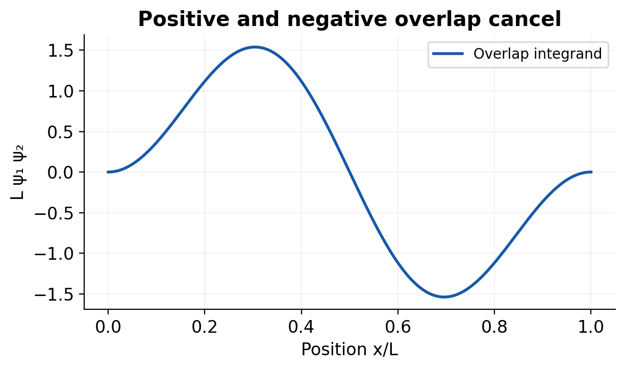
The average energy is |c1|²E1 + |c2|²E2. Its value need not equal either possible measurement result. Position density also contains cross terms whose time dependence follows the relative energy phase.
A common shortcut is valid only for the stated question: orthogonality removes cross terms from the full normalisation and energy expectation in this energy basis, but not from the local position density. Keep coherent amplitudes until the relevant operation has been performed.
Worked Problem 1.34: Equal Energy-State Superposition
Problem: A normalised state has equal amplitude magnitudes in box levels n = 1 and n = 2. For L = 1.00 nm, find energy probabilities and mean energy.
Model / approach: Orthogonal energy states have probabilities equal to squared coefficient magnitudes.
Step 1: Equal weights and normalisation give P(E1) = P(E2) = 1/2.
Step 2: Mean energy = (E1 + E2)/2 = 2.5E1.
Answer: Each energy occurs with probability 0.5000; ⟨E⟩ ≈ 0.9401 eV.
Check: The mean need not appear as a single energy measurement. The local position density of a coherent superposition includes interference terms.
29. What the Confinement Model Explains and Omits
Confinement connects a smaller permitted length with larger energy scales. It helps organise thinking about quantum wells, nanoscale structures and localised particles. The wavelength and level scales explain why microscopic dimensions can matter strongly to electronic behaviour.
Real barriers are finite and real materials have interactions, lattice potentials and often an effective rather than bare mass. In more than one dimension, geometry introduces further quantum numbers and degeneracies. These changes require a model beyond the one-dimensional infinite well.
At sufficiently high quantum number, probability averaged over many short oscillations approaches a classical-looking spatial average for this simple box. This correspondence concerns a coarse-grained distribution; it does not turn one exact standing-wave state into a known classical trajectory.
For a derivation answer, state the potential and domain, apply both wall conditions, reject the zero state, normalise, give the energy spectrum and interpret its dependence on mass and width. A list of final formulas without those steps misses the physical reason for quantisation.

Worked Problem 1.35: Confinement Scaling Without Constants
Problem: For the same particle and state index, one box is narrowed from 2.00 nm to 0.500 nm. Find the energy ratio.
Model / approach: En is inversely proportional to L² at fixed n and mass.
Step 1: Width ratio Lold/Lnew = 2.00/0.500 = 4.00.
Step 2: Enew/Eold = 4.00².
Answer: The narrower box has 16 times the energy.
Check: At fixed width, increasing mass by the same factor would instead reduce the energy. Identify what stays fixed before taking ratios.
30. Quantum Revision: Connect the Eight Syllabus Topics
The logical sequence is classical limitation → matter wavelength → experimental diffraction → localised packet → uncertainty → wavefunction probability → wave equation → boundary-selected energies. Each step addresses a different question: evidence, kinematics, statistics or dynamics.
For wave problems, identify whether frequency is ordinary ν or angular ω. For numerical work, start with λ = h/p and only then select non-relativistic or relativistic momentum. For Davisson-Germer, state the angle convention before applying Bragg’s law.
For probability, normalise over the correct support and integrate the squared modulus. For a stationary state, density can be time independent while phase evolves. For a box, n begins at one and energy is proportional to n², not n.
Uncertainty constrains distribution spreads, not just experimental care. It permits zero average momentum. A phase velocity may exceed c without transporting a signal at that speed. Matter waves can propagate in vacuum. These distinctions prevent several common but misleading short answers.
Branch reading rule. Sections 1–30 cover the complete quantum unit used by CE, ME, ECE, EE, CSE, BT and TX. AG prescribes the core wave/Schrödinger/box topics; additional diffraction and uncertainty lessons are enrichment. CH uses this quantum material in Unit III.
31. [CH] Atomic Structure and Material Description
For CH, Unit I begins with atomic structure and the structure-property connection. An atom contains a small positive nucleus and electrons occupying quantum states. Atomic number gives proton count; mass number gives protons plus neutrons. Isotopes share atomic number but differ in neutron count.
Valence electrons strongly influence bonding and hence electrical, mechanical and thermal behaviour. A material property cannot be inferred from atomic mass alone. Bond type, atomic arrangement, defects, temperature and microstructure all contribute.
A crystal has a repeating long-range arrangement described using a lattice and basis. An amorphous solid lacks that long-range periodic order, although it can retain local atomic organisation. A grain is one crystal region in a polycrystalline material; grain boundaries separate differently oriented regions.
Structure is described at several scales: electronic bonding, atomic packing, defects/grains and the macroscopic component. This unit introduces the ideal structures and elastic measures before more specialised process-material behaviour.
Electronic arrangement and property trends. An orbital label describes a quantum state rather than a small electron moving on a drawn circular track. Electron occupancy and the availability of outer states influence whether atoms tend to share, transfer or delocalise valence charge. The resulting bond environment influences spacing and resistance to displacement. Material processing can change grains, phases and defects while leaving the elemental atomic number unchanged. This is why a complete structure-property explanation names both bonding and atomic arrangement, rather than attributing every measured property to one isolated atom.
Shells and occupation. Principal shell n can hold at most 2n² electrons when all its orbital states are counted. Pauli exclusion allows at most two electrons with opposite spins in one spatial orbital. Ground-state filling follows the available orbital energies, while Hund’s rule favours single occupation of equal-energy orbitals before pairing. For example, neutral sodium has configuration 1s² 2s² 2p⁶ 3s¹; its outer electron is relevant to ionic bonding. Shell-capacity rules do not mean every atom fills an entire shell before any higher-n orbital can be occupied, because orbital energies depend on the atom.
| Quantity | Meaning |
|---|---|
| Atomic number Z | Protons; electrons in a neutral atom |
| Mass number A | Protons + neutrons |
| Valence electrons | Outer electrons important to bonding |
| Crystal lattice + basis | Periodic positions plus atomic motif |
Worked Problem 1.36: Atomic Number and Isotope Count
Problem: A neutral atom is written with atomic number 26 and mass number 56. Find proton, electron and neutron counts.
Model / approach: Atomic number fixes protons; neutrality fixes electrons.
Step 1: Protons = 26; electrons = 26.
Step 2: Neutrons = 56 – 26.
Answer: 26 protons, 26 electrons and 30 neutrons.
Check: An isotope changes neutron count while retaining atomic number. Ionisation changes electron count, not the number of protons in the element.
32. [CH] Ionic, Covalent and Metallic Bonding
Ionic bonding: Electron transfer produces oppositely charged ions whose electrostatic attraction helps bind the solid. Charge neutrality and ion size influence the structure. Ionic solids are often stiff and brittle; an insulating solid can conduct when ions become mobile under suitable conditions.
Covalent bonding: Atoms share electrons in directional bonds. The directionality constrains local geometry and can produce strong networks, such as diamond or silicon. Properties vary widely: bonding alone does not imply every covalent material has identical conductivity or hardness.
Metallic bonding: Valence electrons are delocalised through a lattice of positive ion cores. This supports electrical/thermal conduction and nondirectional bonding. Atomic planes can rearrange through deformation mechanisms, explaining why many metals are ductile rather than brittle.
Bond energy and equilibrium separation help explain elastic response. Stretching slightly from equilibrium produces a restoring force; temperature and composition can modify the response. Actual materials can exhibit mixed bonding rather than fitting one perfectly pure category.
Bond-energy view of small elastic displacement. A schematic pair potential has a minimum at an equilibrium separation r0. At that point the attractive and repulsive contributions balance, so the net force is zero. The restoring force is related to the slope of potential energy. For a small displacement, the curvature near the minimum gives an approximately linear restoring response. A steeper curvature corresponds to a larger local stiffness, although converting a pair potential into a bulk modulus also requires crystal geometry and bonding directions. Bond strength, equilibrium distance and elastic stiffness are related but distinct measures.
| Bond | Electron Picture | Typical Implication |
|---|---|---|
| Ionic | Transfer and charged ions | Strong attraction; often brittle |
| Covalent | Directional sharing | Geometry-sensitive networks |
| Metallic | Delocalised electrons | Conduction and often ductility |
33. [CH] Unit Cells and Lattice Parameters
A unit cell repeats by translation to build a crystal. Lattice parameters are the edge lengths a,b,c and inter-edge angles. For a cubic cell, a = b = c and all angles are 90°. HCP uses a hexagonal description with basal parameter a and axial parameter c.
An atom at a conventional cubic corner is shared by eight cells and contributes 1/8 to one cell. A face-centred atom is shared by two cells and contributes 1/2. A body-centred atom belongs completely to one cell. Count shared fractions before assigning atoms per cell.
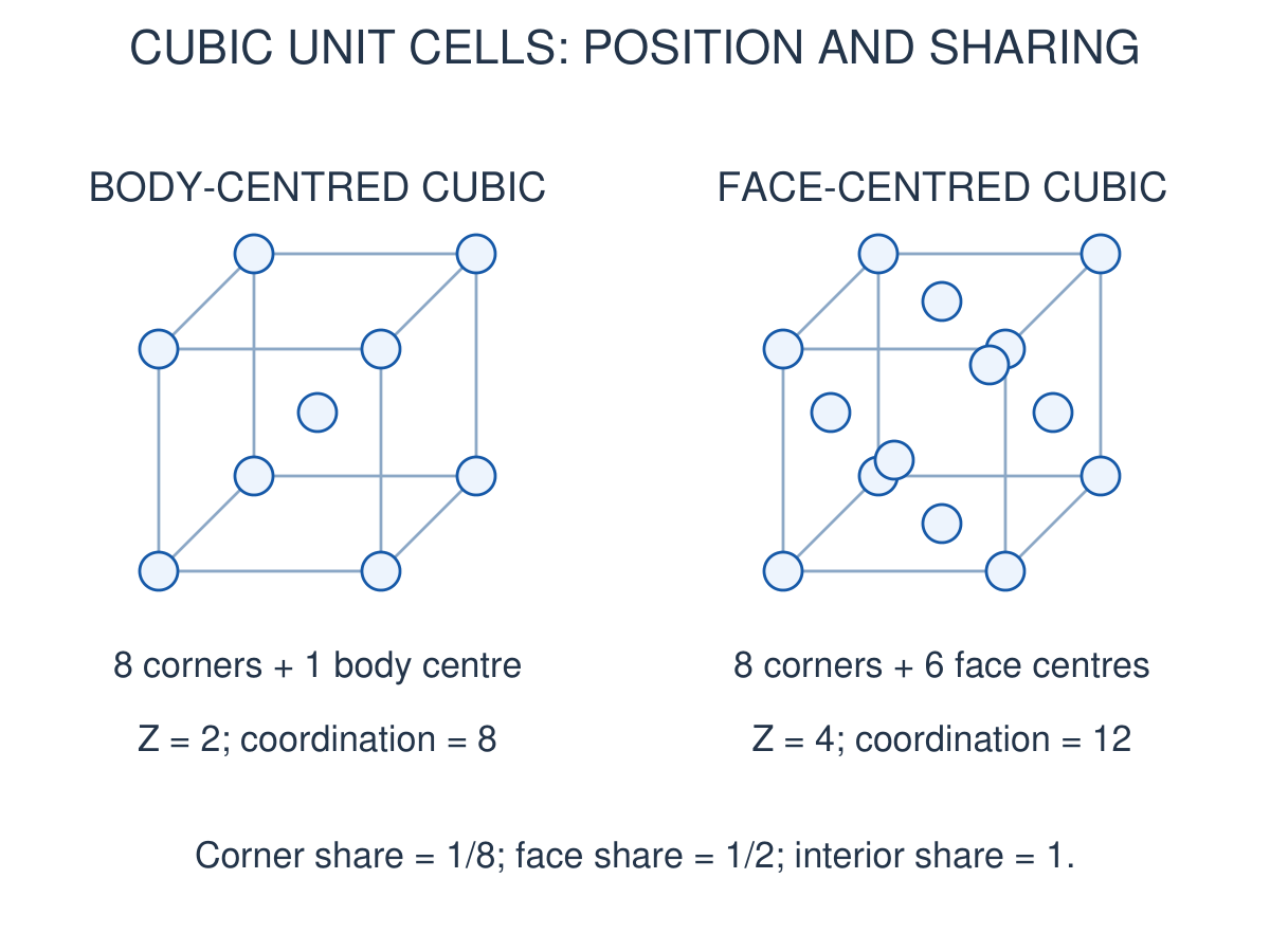
Coordination number counts nearest neighbours, not atoms per unit cell. Atomic packing factor (APF) is ideal hard-sphere volume inside a chosen cell divided by that cell’s volume. It is not the mass density and must not include spheres extending outside the cell without the proper sharing fractions.
The lattice parameter is not always the nearest-neighbour distance. Derive the contact direction for each structure: a cube edge, body diagonal or face diagonal. A memorised formula without its geometry can be applied to the wrong structure.
Count a cell without double-counting. Draw one chosen cell and mark which sites lie on a corner, edge, face or interior. A corner belongs to eight neighbouring cubic cells; an edge-centred site, if present, belongs to four; a face site belongs to two. Sum these fractions. Then compute the cell volume from the same geometric convention. For a cubic cell the volume is a³, not the sum of sphere volumes. The latter is used only in a separate packing calculation. Boundary sharing is a counting device for an extended crystal, not a claim that an atom is physically split into pieces.
34. [CH] BCC, FCC and HCP Packing
BCC: Eight corners plus one body centre give Z = 8/8 + 1 = 2 atoms per conventional cubic cell. Contact along the body diagonal gives √3 a = 4r. Its nearest-neighbour coordination is 8 and ideal APF is π√3/8 ≈ 0.680.
FCC: Eight corners and six face centres give Z = 8/8 + 6/2 = 4. Contact along a face diagonal gives √2 a = 4r. Coordination is 12 and ideal APF is π/(3√2) ≈ 0.740. FCC is a close-packed arrangement with ABCABC layer sequence.
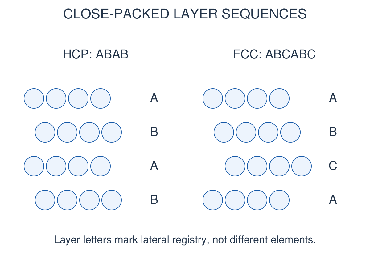
HCP: Ideal close-packed layers follow ABAB rather than FCC’s ABCABC sequence. Coordination is 12, ideal c/a = √(8/3) ≈ 1.633 and APF is approximately 0.740. Actual HCP materials can depart from the ideal axial ratio.
For the conventional full hexagonal prism, the atom count is 6 and the volume is (3√3/2)a²c. A smaller primitive hexagonal cell can use 2 atoms and one-third that volume. Either convention gives the same density when atom count and volume are paired consistently.
Ideal HCP axial-ratio derivation. Take three mutually touching base-layer spheres whose centres form an equilateral triangle of side a = 2r. The next-layer sphere touches all three. The horizontal distance from the triangle centre to a vertex is a/√3. If h is the separation between adjacent A and B centre planes, the contact distance gives a² = h² + a²/3. Hence h = a√(2/3). The repeat distance from one A layer to the next is c = 2h, giving c/a = √(8/3). The result relies on equal hard spheres and ideal contact geometry.
| Structure | Z / CN | Ideal Geometry / APF |
|---|---|---|
| BCC | 2 / 8 | 4r = √3a; 0.680 |
| FCC | 4 / 12 | 4r = √2a; 0.740 |
| HCP full prism | 6 / 12 | a = 2r; ideal c/a 1.633; 0.740 |
Worked Problem 1.37: BCC Radius from Lattice Parameter
Problem: An ideal BCC material has cubic lattice parameter 0.2866 nm. Find atomic hard-sphere radius and atoms per cell.
Model / approach: Atoms touch along the body diagonal; count shared corner sites.
Step 1: √3a = 4r, so r = √3a/4.
Step 2: Z = 8 × (1/8) + 1 = 2.
Answer: r ≈ 0.1241 nm; Z = 2.
Check: Coordination number is 8, not 2. Atoms per cell and nearest-neighbour count describe different properties.
Worked Problem 1.38: FCC Lattice Parameter
Problem: An ideal FCC hard-sphere radius is 0.128 nm. Find a and coordination number.
Model / approach: Contact follows a face diagonal.
Step 1: √2a = 4r, giving a = 2√2r.
Step 2: FCC has 12 nearest neighbours.
Answer: a ≈ 0.362 nm; coordination number 12.
Check: Using the BCC body-diagonal formula would give a different structure. The specified contact geometry determines the relation.
Worked Problem 1.39: Ideal HCP Axial Ratio
Problem: An ideal HCP structure has basal parameter a = 0.320 nm. Find c and the hard-sphere radius.
Model / approach: Use ideal c/a = √(8/3) and a = 2r.
Step 1: c = 1.632993 × a.
Step 2: r = a/2.
Answer: c ≈ 0.5226 nm; r = 0.160 nm.
Check: Actual HCP materials need not have the ideal axial ratio. Use a supplied measured ratio instead when the problem provides one.
Worked Problem 1.40: Derive BCC Packing Factor
Problem: Show the ideal BCC packing factor using Z = 2 and a = 4r/√3.
Model / approach: Divide the sphere volume assigned to the cell by a³.
Step 1: Sphere volume = 2 × (4πr³/3).
Step 2: Cell volume = (4r/√3)³; take their ratio.
Answer: APF = π√3/8 ≈ 0.6802.
Check: APF is dimensionless. It does not equal the mass density and does not count coordination neighbours.
35. [CH] Crystal Density and Structure Calculations
Mass density is cell mass divided by cell volume. If Z atoms of molar mass M belong to a cell, mass per cell is ZM/NA. For a cubic cell, ρ = ZM/(NAa³). Use M in kg/mol and a in metres to obtain kg/m³.
When M is in g/mol and a in centimetres, the same formula gives g/cm³. Mixing a in nm with a volume assumed to be cm³ creates errors of many powers of ten. Record the unit conversion before cubing the lattice parameter.
For a specimen volume V, the ideal number of cells is V/a³ and atom count is ZV/a³ for a cubic perfect-crystal model. Surface truncation, vacancies, porosity and multiple phases are not included in this simple estimate.
Density alone does not always identify a unique crystal structure because composition, defects and temperature also matter. Structure calculations should specify the supplied model and check whether the resulting scale is plausible. One g/cm³ equals 1000 kg/m³.
Check the density formula by dimensions. The molar mass M divided by Avogadro constant has units of mass per atom. Multiplication by Z gives mass assigned to one cell, and dividing by cell volume gives mass per volume. If measured density and M are known, Z = ρNAa³/M can test a proposed cubic model, but the result must be interpreted with composition and defect assumptions. A value near an integer may support the model; density alone is not a direct image of atomic positions. Thermal expansion changes a and therefore the density even without changing Z.
Worked Problem 1.41: Density of a Supplied BCC Model
Problem: Use BCC Z = 2, a = 0.2866 nm and molar mass M = 55.845 g/mol. Find ideal density.
Model / approach: ρ = ZM/(NA a³), with consistent SI units.
Step 1: M = 0.055845 kg/mol; a = 2.866 × 10^-10 m.
Step 2: Find cell mass 2M/NA and divide by a³.
Answer: ρ ≈ 7878 kg/m³ = 7.878 g/cm³.
Check: The estimate assumes an ideal fully dense structure and the supplied lattice parameter. Porosity and defects can alter measured bulk density.
Worked Problem 1.42: FCC Density and Units
Problem: Use FCC Z = 4, a = 0.3615 nm and M = 63.546 g/mol. Find density in g/cm³.
Model / approach: Use either one consistent SI route or one consistent centimetre route.
Step 1: In SI, M = 0.063546 kg/mol and a = 3.615 × 10^-10 m.
Step 2: Evaluate 4M/(NA a³), then divide kg/m³ by 1000.
Answer: ρ ≈ 8.935 g/cm³.
Check: Convert the lattice parameter before cubing it. A cubic volume conversion contains the cube of the length conversion factor.
Worked Problem 1.43: Number of Atoms in a Crystal Volume
Problem: An ideal BCC crystal has a = 0.300 nm and specimen volume 1.00 mm³. Estimate its cell and atom counts.
Model / approach: Ncells = V/a³; Natoms = Z Ncells.
Step 1: V = 1.00 × 10^-9 m³ and a = 3.00 × 10^-10 m.
Step 2: Divide by a³, then multiply by Z = 2.
Answer: Cells ≈ 3.704 × 10^19; atoms ≈ 7.407 × 10^19.
Check: This bulk ideal-crystal estimate neglects surface truncation and vacancies. Counting all visible corner spheres as whole atoms would overcount.
36. [CH] Stress, Strain and Elastic Response
Engineering normal stress is force divided by original cross-sectional area: σ = F/A0. Tensile stress stretches a specimen; compressive stress shortens it under the chosen sign convention. Stress has units N/m² = Pa. One MPa equals one N/mm².
Engineering longitudinal strain is ε = ΔL/L0. It is dimensionless and may be expressed as a fraction, percent or microstrain. A value 0.001 is 0.1%, not 1%. Keep original and deformed dimensions distinct when a problem asks for engineering rather than true measures.
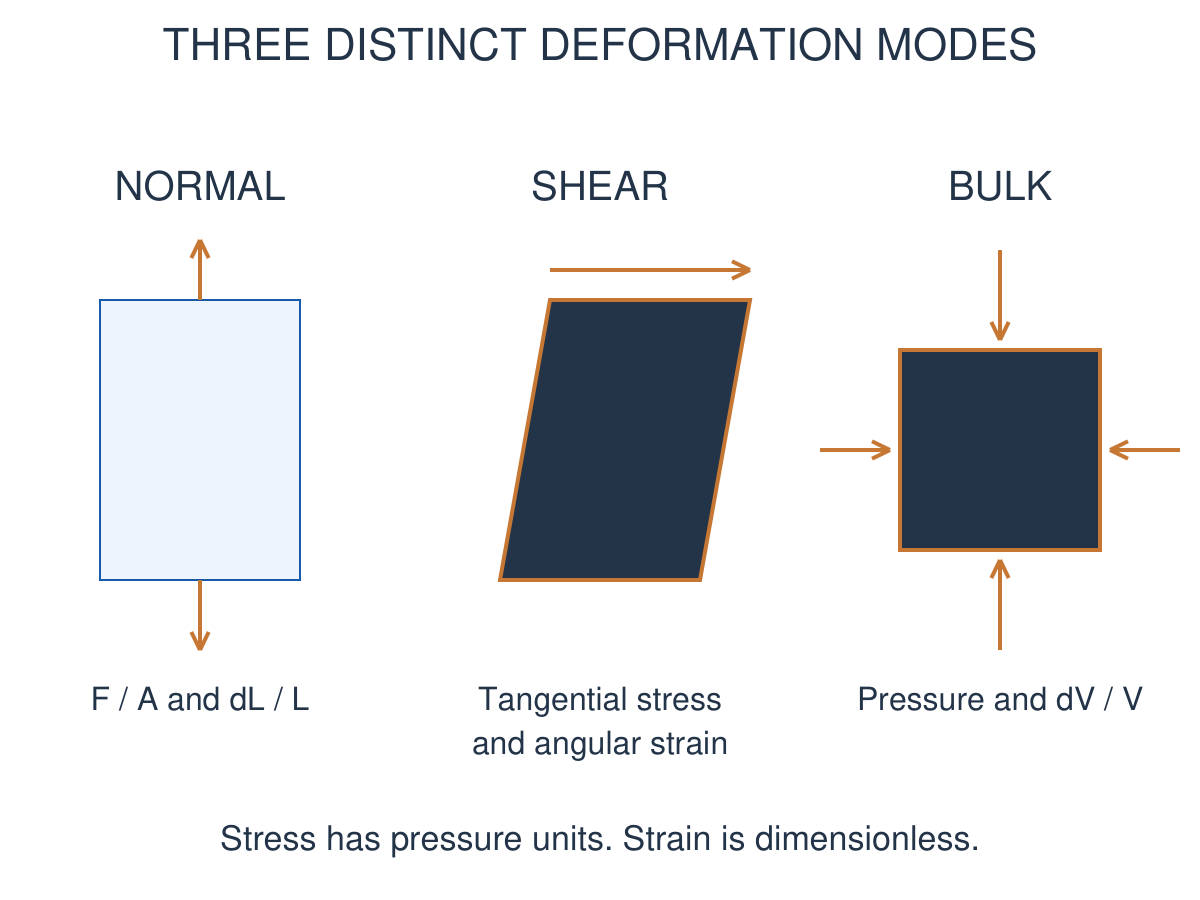
Shear stress is tangential force divided by the relevant area. For a small simple shear, strain γ ≈ lateral displacement/height ≈ shear angle in radians. Volumetric strain is ΔV/V; its sign depends on whether compression is represented as negative or by a positive magnitude.
Elastic deformation is recovered on unloading within the relevant regime. Linear elasticity is the more restrictive region where stress is proportional to strain. Elastic does not automatically mean exactly linear up to every load.
Separate specimen stiffness from material stiffness. Two wires made from the same linear elastic material can extend by different amounts under the same force. The material has the same Young modulus, while the component relation ΔL = FL/(AY) depends on length and area. A longer wire is more compliant and a thicker wire is less compliant. Stress-strain coordinates remove these simple geometry factors so that a constitutive material response can be compared. The distinction is important when a process component is redesigned without changing its material.
Worked Problem 1.44: Engineering Tensile Stress
Problem: A tensile force 5000 N acts on original cross-sectional area 25.0 mm². Find engineering stress.
Model / approach: σ = F/A0; 1 N/mm² = 1 MPa.
Step 1: σ = 5000/25.0 = 200 N/mm².
Step 2: Equivalently A0 = 25.0 × 10^-6 m² and σ = 2.00 × 10^8 Pa.
Answer: σ = 200 MPa.
Check: The area is the original area for engineering stress. Use current area only when the requested definition is true stress.
Worked Problem 1.45: Strain, Percent and Microstrain
Problem: A 2.00 m gauge length extends by 0.500 mm. Find longitudinal strain, percent strain and microstrain.
Model / approach: Convert extension to the same length unit as the gauge length.
Step 1: ε = 0.000500/2.00 = 0.000250.
Step 2: Percent = 100ε; microstrain = 10^6 ε.
Answer: ε = 2.50 × 10^-4 = 0.0250% = 250 microstrain.
Check: Strain is dimensionless. A numerical fraction and the percentage written from it differ by a factor of 100.
37. [CH] Young, Bulk and Shear Moduli
Young modulus Y is normal stress divided by longitudinal strain in a uniaxial linear elastic test: Y = σ/ε = FL0/(A0ΔL). It measures stiffness of the material, while a component’s extension also depends on its dimensions.
Bulk modulus K measures resistance to volume change under hydrostatic pressure: K = -Δp/(ΔV/V) for a sufficiently small change. With compression magnitudes, K = Δp/|ΔV/V|. The minus sign makes K positive for ordinary stable materials.
Shear modulus G is shear stress divided by shear strain in the linear regime: G = τ/γ. It measures resistance to shape change rather than direct hydrostatic volume compression. All three moduli have pressure units.
Poisson ratio νP is minus transverse strain divided by axial strain in a uniaxial test. For a homogeneous isotropic linear elastic material, Y = 2G(1 + νP) = 3K(1 – 2νP) and Y = 9KG/(3K + G). Do not impose these isotropic formulas blindly on direction-dependent single-crystal properties.
Using an isotropic identity safely. Given Y and νP, calculate G and K only after confirming the stated isotropic linear assumptions. Positive moduli provide a useful stability check in an ordinary elastic model. As νP approaches one half from below at fixed finite Y, K grows strongly, representing resistance to volume change; this does not force G to diverge. A polycrystalline aggregate may be approximated as isotropic under suitable conditions, whereas a single crystal can require directional elastic constants. State the approximation instead of treating one scalar modulus as a complete description of every crystal.
Worked Problem 1.46: Extension of a Linear Elastic Wire
Problem: A wire has L0 = 2.00 m, A0 = 10.0 mm² and Y = 200 GPa. A 1000 N axial force stays in the linear elastic regime. Find extension.
Model / approach: Rearrange Y = FL0/(A0 ΔL).
Step 1: A0 = 10.0 × 10^-6 m²; Y = 2.00 × 10^11 Pa.
Step 2: ΔL = FL0/(A0Y).
Answer: ΔL = 1 mm.
Check: The relation assumes a uniform uniaxial specimen and small linear elastic strain. A load beyond the stated regime requires a different constitutive model.
Worked Problem 1.47: Young Modulus from a Test Point
Problem: A uniaxial linear test gives stress 100 MPa at strain 0.000500. Find Y.
Model / approach: Use the slope σ/ε in the specified linear elastic region.
Step 1: Convert 100 MPa to 1.00 × 10^8 Pa.
Step 2: Y = 1.00 × 10^8 / 5.00 × 10^-4.
Answer: Y = 2.00 × 10^11 Pa = 200 GPa.
Check: The ratio at an arbitrary nonlinear/plastic point is not automatically the Young modulus. The supplied linear-regime condition matters.
Worked Problem 1.48: Bulk Modulus Under Compression
Problem: An increase in hydrostatic pressure of 50.0 MPa causes a fractional volume decrease of 0.000500. Find K.
Model / approach: Use positive pressure and positive compression magnitude.
Step 1: K = Δp/|ΔV/V|.
Step 2: K = 50.0 × 10^6 / 5.00 × 10^-4.
Answer: K = 1.00 × 10^11 Pa = 100 GPa.
Check: With signed volumetric strain, ΔV/V is negative and the defining formula contains a minus sign. Both conventions give a positive modulus here.
Worked Problem 1.49: Shear Modulus from Angular Strain
Problem: A small shear stress of 20.0 MPa produces shear angle 0.000250 rad. Find G.
Model / approach: For small simple shear, γ is approximately the angle in radians.
Step 1: G = τ/γ = 20.0 × 10^6 / 2.50 × 10^-4.
Step 2: Express the result in GPa.
Answer: G = 8.00 × 10^10 Pa = 80.0 GPa.
Check: Degrees cannot be substituted directly into the small-angle strain formula. Shear strain describes shape change rather than hydrostatic volume compression.
38. [CH] Stress-Strain Curve and Unit Revision
The initial slope of a uniaxial stress-strain curve gives Young modulus in its linear elastic region. The proportional limit, elastic limit, yielding, maximum engineering stress and fracture are different features. Their exact appearance depends on the material and test conditions.
A ductile specimen can undergo substantial permanent strain before fracture. A brittle specimen fractures with comparatively little plastic strain. High stiffness, high strength and high toughness are different properties; one should not be substituted for another in an explanation.
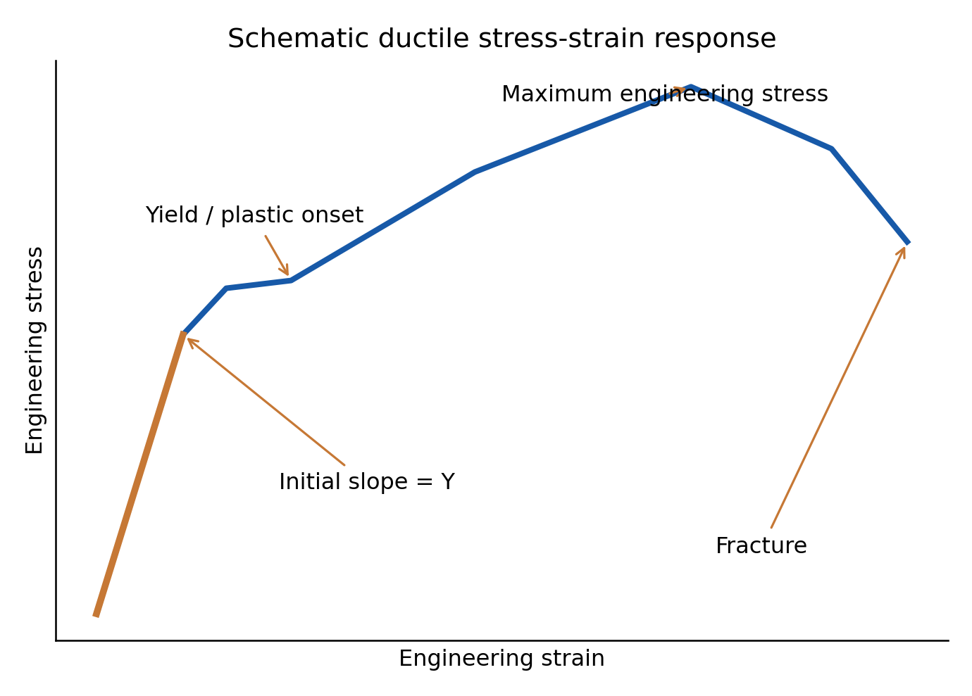
For uniaxial linear loading, elastic strain-energy density is u = σε/2 = σ²/(2Y). It is the area under the linear stress-strain segment and has units J/m³. The full area to fracture describes a different energy measure and cannot be found from the initial slope alone.
Revision path: Atomic/valence structure → bonding → crystal geometry → sharing/counting → density → stress/strain → modulus and elastic response. For every calculation state the material model, unit-cell convention or loading mode before substituting values.
Read a curve before calculating an energy. Identify whether the horizontal axis is fractional strain or percent strain, and whether the vertical axis is stress or force. The area under a stress-strain graph has energy-per-volume units because strain is dimensionless. The area under a force-extension graph instead has energy units. For a linear elastic segment, the triangular area is σε/2. Beyond that region, use the actual curve rather than extending the initial straight line indefinitely. Yield strength, ultimate engineering strength, fracture strain and elastic modulus answer different design questions.
Worked Problem 1.50: Check Isotropic Modulus Relations
Problem: For a homogeneous isotropic linear elastic material, Y = 200 GPa and Poisson ratio νP = 0.250. Find G and K.
Model / approach: Use the isotropic relations only under the supplied assumptions.
Step 1: G = Y/[2(1 + νP)] = 200/2.5 = 80.0 GPa.
Step 2: K = Y/[3(1 – 2νP)] = 200/1.5 GPa.
Answer: G = 80.0 GPa; K ≈ 133.3 GPa.
Check: Check Y = 9KG/(3K + G). A direction-dependent single crystal cannot be reduced to these isotropic relations without an appropriate model.
COMPLETE EXPLANATIONS FOR EXAM ANSWERS
Explain How Electron Diffraction Verifies De Broglie’s Hypothesis
De Broglie relates a particle’s wavelength to its momentum, λ = h/p. To test this relation, use an electron beam whose accelerating potential supplies a known kinetic-energy scale and an ordered crystal whose plane spacing supplies an independent diffraction scale. A successful test compares two numerical wavelengths rather than merely observing a detector signal.
A heated filament produces electrons, accelerating/focusing electrodes prepare the beam and a nickel crystal scatters it in vacuum. A movable collector records intensity as a function of direction for selected accelerating voltages. Vacuum reduces collisions that would disturb the intended beam-crystal interaction. The controlled variables and measured collector angle/current must be identified in the diagram.
A strong introductory example occurs near 54 V and a collector angle of 50° under the stated geometry. Convert that angle using 2θ + φ = 180° to obtain a glancing angle of 65°. With the supplied plane spacing 0.091 nm, first-order Bragg interference gives λ = 2d sinθ, approximately 0.165 nm. The non-relativistic electron momentum inferred from 54 V gives approximately 0.167 nm through h/√(2me eV).
The agreement supports the wave character of electrons and the predicted momentum-wavelength relation. The collector peak indicates enhanced intensity from constructive interference, not a new energy source. The conclusion depends on the crystal geometry and model assumptions; it is not justified by inserting an arbitrary distance or confusing the glancing angle with the detector angle.
Obtain the Stationary Equation and Explain Its Meaning
For a non-relativistic particle, the time-dependent equation is iħ∂Ψ/∂t = [-ħ²∂²/(2m∂x²) + U]Ψ. A free plane-wave component motivates the operator form: temporal differentiation supplies ħω and spatial second differentiation supplies ħ²k²/(2m), consistent with E = p²/(2m), E = ħω and p = ħk. The dynamical equation remains a postulate rather than a theorem of classical mechanics.
For a time-independent U(x), set Ψ = ψ(x)T(t), substitute and divide by the product. The resulting temporal expression iħT′/T equals the spatial expression -ħ²ψ″/(2mψ) + U. Because the variables are independent, their common value is the separation constant E. Integration of the time equation gives T = exp(-iEt/ħ).
The spatial equation is -ħ²ψ″/(2m) + Uψ = Eψ. It must be solved over the stated region with appropriate matching and wall conditions. Normalisability and those conditions decide which energies describe allowed bound states. Different conditions may produce continuous scattering spectra instead.
For a single energy eigenstate, the phase factor has unit modulus, so |Ψ|² = |ψ|² is stationary. This does not imply zero kinetic energy or a fixed known particle position. Superpositions of different energies generally have evolving relative phases and time-dependent position densities. Explain the phase and density separately when interpreting a stationary solution.
Derive the One-Dimensional Infinite-Well States and Spectrum
Choose a well from x = 0 to x = L, with zero interior potential and infinite exterior barriers. The state is zero outside, and the wall values satisfy ψ(0) = ψ(L) = 0. Inside, the TISE becomes ψ″ + k²ψ = 0, where k² = 2mE/ħ² for the positive-energy solutions.
The general interior solution is A sin(kx) + B cos(kx). The left boundary makes B zero. A nonzero state at the second boundary requires sin(kL) = 0, hence k = nπ/L. The zero index gives a zero wavefunction and cannot be normalised, so use n = 1,2,3,… . The quantisation therefore follows from the simultaneous wall conditions.
Normalisation gives 1 = |A|²∫ from 0 to L sin²(nπx/L)dx = |A|²L/2. A convenient amplitude is √(2/L). Substituting the allowed k into ħ²k²/(2m) yields En = n²h²/(8mL²). The ground energy is positive, successive gaps increase, and a reduction in width raises every level as L^-2.
The density is (2/L)sin²(nπx/L). Its zeros at the walls and its n – 1 internal nodes follow directly from the sine. Probability in any interval comes from integrating this density; the mean position is L/2 by symmetry. The mean momentum can be zero while the mean-square momentum is positive. These statistical statements explain why the state is not a classical particle at rest.
A complete answer ends with the model limits: real barriers can permit penetration, interactions can change the potential and more dimensions require further quantum numbers. The ideal well isolates the connection between confinement, boundary conditions and discrete energies.
[CH] Connect Crystal Geometry with Elastic Measurements
Begin with the bonding picture and the repeating crystal geometry. Ionic transfer, covalent sharing and metallic delocalisation describe different electronic environments. Their force-separation behaviour, directionality and atomic arrangement affect stiffness and deformation. A unit-cell drawing provides geometric information, while an elastic test measures response under a defined loading mode.
For BCC, corner sharing and one interior site give two atoms per cubic cell; contact along the body diagonal gives 4r = √3a. For FCC, corner and face sharing give four atoms, and contact along the face diagonal gives 4r = √2a. Coordination counts nearest neighbours and differs from this atom count. HCP has the same ideal close-packing fraction as FCC but an ABAB sequence instead of ABCABC.
Use the same cell convention for mass and volume. A cubic density is ZM/(NAa³); the full HCP prism instead pairs six atoms with volume (3√3/2)a²c. Convert length before cubing it and molar mass before combining SI quantities. The resulting density is a mass-per-volume property, not the dimensionless packing fraction.
For a small uniaxial linear test, engineering stress is F/A0, strain is ΔL/L0 and their ratio is Young modulus. Bulk modulus describes hydrostatic volume change and shear modulus describes tangential shape change. The curve’s initial slope, yielding and fracture identify different properties. State whether isotropy and linearity are assumed before using relations among Y, K, G and Poisson ratio.
FORMULA SHEET WITH MODEL CONDITIONS
| Quantum Relation | Condition / Meaning |
|---|---|
| λ = h/p | Use the appropriate momentum model |
| λ = h/√(2mK) | Non-relativistic kinetic energy |
| K gain = |q|V | Stated accelerating work; include initial K |
| nλ = 2d sinθ | θ measured from lattice planes |
| vp = ω/k; vg = dω/dk | State dispersion and energy convention |
| σx σp ≥ ħ/2 | Same-direction standard deviations |
| P(a,b) = ∫|ψ|² dx | Use a normalised state and correct support |
| iħ ∂Ψ/∂t = HΨ | Non-relativistic time evolution |
| Hψ = Eψ | Time-independent potential; spatial boundary conditions |
| ψn = √(2/L) sin(nπx/L) | Infinite well 0 < x < L; n ≥ 1 |
| En = n²h²/(8mL²) | Infinite well, non-relativistic particle |
| Photon energy = |Ef – Ei| | Assume a permitted radiative transition |
| Materials Relation | Condition / Meaning |
|---|---|
| BCC: 4r = √3a | Cubic body-diagonal contact |
| FCC: 4r = √2a | Cubic face-diagonal contact |
| Ideal HCP c/a = √(8/3) | Equal hard spheres; ideal stacking |
| Density = ZM/(NA Vcell) | Pair atom count with the same cell volume |
| σ = F/A0; ε = ΔL/L0 | Engineering uniaxial measures |
| Y = σ/ε | Uniaxial linear elastic regime |
| K = -Δp/(ΔV/V) | Small hydrostatic volume change |
| G = shear stress / shear strain | Small linear simple shear |
| Y = 2G(1 + νP) | Homogeneous isotropic linear model |
| Y = 3K(1 – 2νP) | Same isotropic assumptions |
Memory check: Use momentum for wavelength, amplitude squared for probability, boundaries for allowed energy, shared fractions for atoms per cell and the correct loading mode for each modulus. A formula is complete only with its model and units.
QUICK REVISION: EXPLAIN AND CONNECT
Can Matter Waves Propagate in Vacuum?
Yes. They are quantum amplitudes rather than mechanical disturbances requiring a material medium.
Which Momentum Formula Should Be Used?
λ = h/p is the starting relation. Use p = mv only in a suitable non-relativistic regime; otherwise use relativistic momentum.
What Did Davisson-Germer Test?
The wavelength inferred from electron diffraction agreed with the wavelength predicted from momentum.
Why Can Phase-Speed Formulas Differ?
The K-only non-relativistic and total-relativistic energy conventions have different phase evolution but consistent free-particle group speed.
Does Zero Average Momentum Mean Rest?
No. Momentum spread and mean-square momentum may be nonzero even when the average is zero.
What Does Normalisation Establish?
Total probability is one over the declared support; it does not by itself determine energy or momentum.
Why Is the Box Ground Energy Nonzero?
The wall conditions make n = 0 the zero function, which cannot be a physical normalised state.
Why Can a Mean Energy Lie Between Levels?
It is an average over possible outcomes of a superposed state, not necessarily one outcome.
| Before Calculating | Question to Resolve |
|---|---|
| Quantum wavelength | Particle, momentum and energy convention? |
| Probability | Correct state, support and normalisation? |
| Crystal structure | Cell geometry and sharing convention? |
| Elastic response | Loading mode, units and linear regime? |
How Do Z and Coordination Differ?
Z counts the fractionally assigned atoms in a chosen unit cell. Coordination counts nearest neighbours.
Are FCC and HCP Equally Packed?
Their ideal hard-sphere APF is the same, but their layer stacking sequences and lattice descriptions differ.
Which Modulus Describes Volume Change?
Bulk modulus measures resistance to hydrostatic volume compression. Young and shear moduli describe different loading modes.
When May Modulus Relations Be Combined?
The simple Y, K, G and Poisson-ratio identities require the stated isotropic linear elastic model.
Why Square the Modulus of the State?
The wavefunction is a complex amplitude. Its squared modulus is nonnegative probability density, which must be integrated over an interval.
Does a Finite Barrier Force Zero Amplitude at Its Edge?
Not generally. Use the matching conditions for the finite potential; an infinite hard wall is a different idealisation.
Why Do BCC and FCC Radius Formulas Differ?
Their nearest-contact directions differ: the body diagonal in BCC and a face diagonal in FCC.
Is High Stiffness the Same as High Strength?
No. Modulus describes the initial elastic slope; strength concerns stresses associated with yielding or failure under specified conditions.