
Course: AKTU B.Tech First Year | Semester I & II
Course Codes: AAS101A–AAS101I | AAS201A–AAS201I
Streams: CSE, EE, ECE, CE, ME, BT, CH, TX & AG
Unit III Overview
Explore quantum information, electromagnetic fields, dielectric and magnetic response, thermal processes, mechanics, fluids and nanoscale physics. Unit III differs across branches: use the branch guide to select your prescribed sections and solved examples.
Topics Covered
| Topic | Pages |
|---|---|
| Quantum computing and communication | 3–8 |
| Electromagnetic fields and waves | 8–12 |
| Dielectric, magnetic and electrical response | 12–16 |
| Thermal physics and heat transfer | 16–20 |
| Mechanics, elasticity and fluid flow | 20–24 |
| Superconductivity and nanomaterials | 24–27 |
| Quantum mechanics and the 1D box | 27–30 |
Learning Outcomes
- Interpret quantum states, gates, entanglement and the purpose of QKD.
- Connect field laws with wave propagation, energy flow and attenuation.
- Explain dielectric, magnetic and electromechanical material response.
- Apply heat, force and fluid-flow balances with stated assumptions.
- Distinguish superconducting regimes and quantised confinement.
Included in These Notes
50 solved problems with methods and physical checks; 37 labelled diagrams; complete derivations; a formula sheet with conditions and answered revision checks.
Study Approach
Choose your route. Read the branch guide for your branch, course codes and Unit III section numbers.
Trace the mechanism. Follow states, fields, force arrows and energy paths in the labelled diagrams.
Practise carefully. Declare the model, convert units and check signs, probabilities and regimes.
Revise actively. Reproduce key derivations and explain why each formula needs its assumptions.
Coverage note: The combined volume supports all nine streams. Its routes are different Unit III syllabuses; the branch guide identifies what each stream must study.
Unit III: Branch and Topic Guide
Find your branch below. Each AAS101/AAS201 pair uses the same within-stream syllabus. The sections listed cover that stream’s actual Unit III; other routes remain optional background.
| Stream / Codes | Official Subject Title | Official Unit III / Sections |
|---|---|---|
| CE — AAS101A / AAS201A | Physics for Sustainable Structural Systems | Mechanics and Fluid Physics — Sections 27–33 |
| ME — AAS101B / AAS201B | Physics of Materials | Thermal Physics — Sections 22–26 |
| ECE — AAS101C / AAS201C | Quantum Physics and Electronic Sensors | Electromagnetic Field Theory — Sections 9–15 |
| EE — AAS101D / AAS201D | Physics of Electrical Engineering Materials | Electromagnetic Field Theory — Sections 9–15 |
| CSE — AAS101E / AAS201E | Quantum Physics and Applications | Quantum Computing and Communication — Sections 1–8 |
| BT — AAS101F / AAS201F | Physics of Materials and Biomaterials | Dielectric and Magnetic Materials — Sections 16–19 |
| CH — AAS101G / AAS201G | Physics of Process Engineering Materials | Fundamentals of Quantum Mechanics — Sections 38–42 |
| AG — AAS101H / AAS201H | Physics of Agricultural Systems and Environment | Superconductivity and Nano-materials — Sections 34–37 |
| TX — AAS101I / AAS201I | Physics of Fibres and Textile Materials | Thermal and Electrical Properties — Sections 20–24 |
CSE: Qubits, states, superposition, entanglement, decoherence, solid-state and photonic realisations, single/multi-qubit gates, cryptography and QKD (1–8).
EE and ECE: Basic field laws, charge continuity, displacement current, Maxwell forms, vacuum/conductor waves, Poynting theory and skin depth (9–15).
BT: Dielectric vectors, susceptibility, polarisation mechanisms and applications; magnetic classes, susceptibility, hysteresis, loss, coercivity, remanence and applications (16–19).
TX: Bands and electrical classes (20), dielectrics/piezoelectricity/ferroelectricity (21), thermodynamic laws and heat transfer/capacity/conductivity (22–24). The restrained-stress extension in 24 and all of 25–26 are ME depth.
ME: All thermal sections 22–26, including expansion, phase change, resistance, enthalpy, entropy, state equations and cooling.
CE: Mechanics and elastic response (27–29), then fluid properties through pipe flow (30–33).
AG: Superconductivity, high-temperature materials, nanomaterial properties, confinement, top-down/bottom-up fabrication and applications (34–37).
CH: The complete quantum-mechanics route is 38–42: classical limitations, matter waves/Davisson-Germer, packets/velocities, uncertainty and applications, both wave equations, probability interpretation and the 1D box. CH follows suffix G from the supplied course scheme.
1. A. Quantum Computation and the Qubit – CSE
Quantum computation processes information encoded in quantum states. A classical bit has a definite logical value zero or one when read. A qubit is a two-level quantum system with a pure state |ψ⟩ = α|0⟩ + β|1⟩, where α and β are generally complex amplitudes and |α|² + |β|² = 1. The basis states are orthonormal.
A computational-basis measurement returns zero with probability |α|² and one with probability |β|². It does not print both amplitudes or all branches of a calculation in one run. Repeated preparations and measurements estimate the probabilities. A physical implementation must provide distinguishable levels, controllable transformations and a readout mechanism.
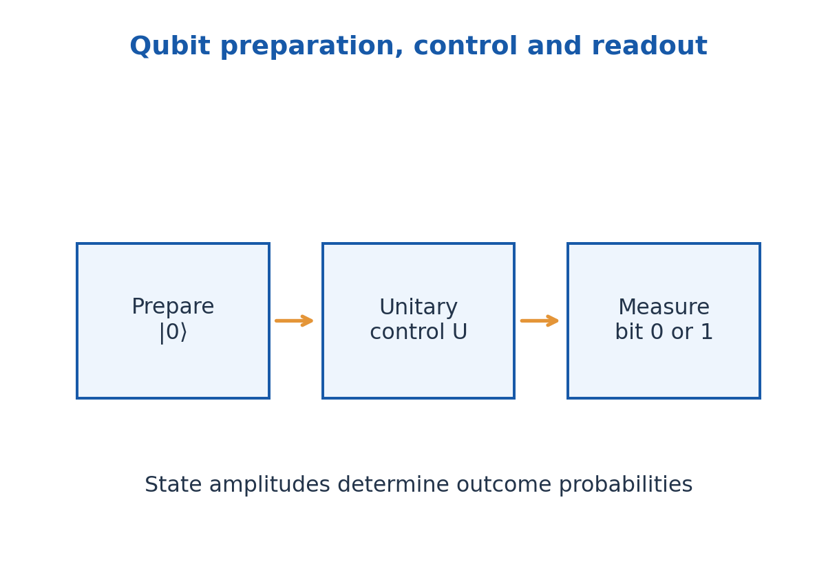
Quantum algorithms exploit interference and, for many tasks, entanglement to change the probability of useful outcomes. A quantum computer is not faster for every problem, and the existence of 2^n amplitudes does not mean 2^n classical answers can be freely read. Encoding, operations, error and readout all constrain a computation.
A circuit model describes preparation, gates and measurement in a specified order. Ideal closed-system gates are unitary and hence reversible; measurement has a different role. Keep the abstract logical state separate from its hardware: a circuit wire represents a qubit’s history, not necessarily a literal conducting wire.
Worked Problem 3.1: Normalise a Qubit
Problem: A state is A(3|0⟩ + 4i|1⟩). Find a positive A and computational-basis probabilities.
Method: Sum squared amplitude magnitudes to one.
Calculation: 1 = A²(9 + 16); A = 1/5.
Answer: A = 0.200; P(0) = 9/25 = 0.360; P(1) = 16/25 = 0.640.
Check: The phase i contributes magnitude one; it is not a negative probability.
2. Superposition, Relative Phase and Measurement
The states |+⟩ = (|0⟩ + |1⟩)/√2 and |-⟩ = (|0⟩ – |1⟩)/√2 have equal zero/one measurement probabilities. They are nevertheless different states because relative phase affects interference and measurements in another basis. A common overall phase multiplying the entire state does not change measurement probabilities.
The Bloch-sphere form of a pure qubit is cos(θ/2)|0⟩ + exp(iφ)sin(θ/2)|1⟩, after removing global phase. The poles represent |0⟩ and |1⟩; equatorial states have equal computational-basis probabilities with different relative phases. Mixed states lie inside the sphere; not every preparation is pure.
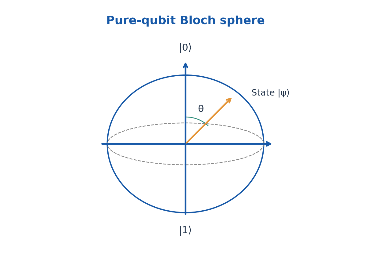
For a projective measurement in an orthonormal basis, the probability is the squared magnitude of the state’s overlap with the selected basis vector. After an ideal measurement with a known outcome, the conditional state is that eigenstate. Repeating the same ideal measurement immediately gives the same outcome.
A coherent superposition is different from an unknown classical mixture with the same zero/one frequencies. Interference can distinguish them. For instance, applying H before measurement makes |+⟩ return zero certainly, whereas a half-zero, half-one classical mixture still gives both results equally.
Worked Problem 3.2: Relative Phase and Measurement Basis
Problem: For |ψ⟩ = (|0⟩ – |1⟩)/√2, find computational-basis probabilities and the outcome after H followed by computational measurement.
Method: The state is |-⟩; H|-⟩ = |1⟩.
Calculation: Before H both amplitudes have squared magnitude 1/2. After H the zero amplitude cancels.
Answer: Initially P(0) = P(1) = 1/2; after H the result is 1 with certainty.
Check: Equal Z-basis probabilities do not imply that |+⟩ and |-⟩ are the same state.
Worked Problem 3.3: Bloch Polar Angle
Problem: A pure qubit is cos(θ/2)|0⟩ + exp(iφ)sin(θ/2)|1⟩ with θ = π/3. Find P(0) and P(1).
Method: P(0) = cos²(θ/2); P(1) = sin²(θ/2).
Calculation: θ/2 = π/6; φ does not affect this measurement basis.
Answer: P(0) = 3/4; P(1) = 1/4.
Check: The polar angle itself is not a probability, and relative phase can matter in another basis.
3. Single-Qubit Gates and Matrix Calculation
In the ordered basis |0⟩, |1⟩, write a state as column (α, β). A gate matrix multiplies this column on the left. X = [[0,1],[1,0]] exchanges the two amplitudes. Z = [[1,0],[0,-1]] changes the relative sign of the |1⟩ component; it does not exchange the measurement probabilities in the computational basis.
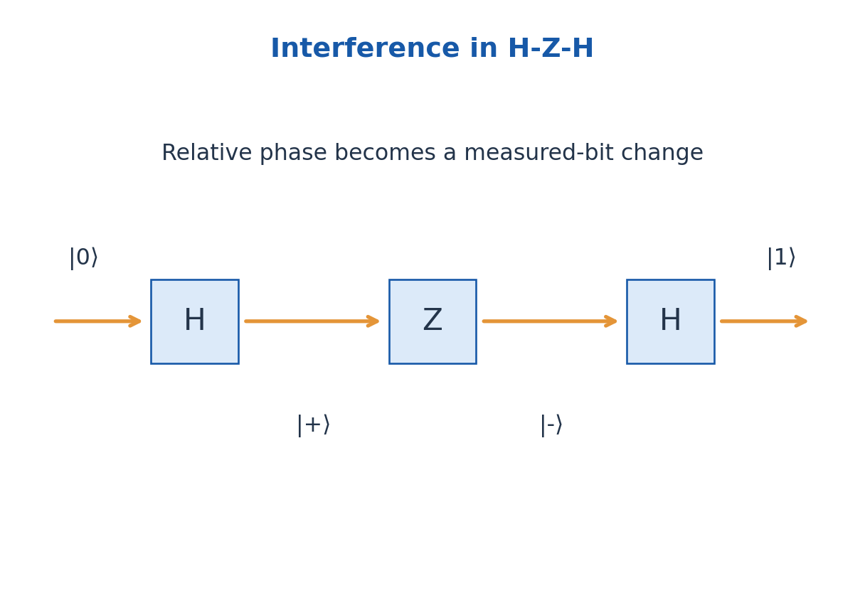
The Hadamard gate is H = (1/√2)[[1,1],[1,-1]]. It maps |0⟩ to |+⟩ and |1⟩ to |-⟩. Since H² = I, applying H twice restores the original state. Applying Z between two H gates can turn an initially hidden relative phase into a change in the final measured bit.
Y = [[0,-i],[i,0]] combines a bit exchange with phase factors. The phase gates S = diag(1,i) and T = diag(1,exp(iπ/4)) alter relative phase. Unitarity U†U = I preserves normalisation; not every matrix is a valid deterministic isolated-system quantum gate.
For a sequence U1 followed by U2, the final state is U2U1|ψ⟩. The rightmost matrix acts first. Gates need not commute: XZ and ZX differ by a sign as matrices, while other orderings can change observable probabilities. State preparation and the measured basis must accompany a numerical answer.
Worked Problem 3.4: H-Z-H Sequence
Problem: Start in |0⟩ and apply H, then Z, then H. Find the final state.
Method: Apply matrices in physical time order to the state.
Calculation: |0⟩ → |+⟩ → |-⟩ → |1⟩.
Answer: Final state |1⟩; computational outcome 1 is certain.
Check: The combined matrix is HZH = X, not three independent measurements.
Worked Problem 3.5: An X Gate on Complex Amplitudes
Problem: Apply X to (|0⟩ + i|1⟩)/√2. Report amplitudes and computational probabilities.
Method: X exchanges the two components.
Calculation: Column (1,i)/√2 becomes (i,1)/√2.
Answer: State (i|0⟩ + |1⟩)/√2; each computational probability remains 1/2.
Check: A state can change while one chosen measurement distribution remains unchanged.
4. Two-Qubit States, CNOT and Entanglement
Two qubits have basis |00⟩, |01⟩, |10⟩, |11⟩ in the declared first-second order. A product state is (a|0⟩ + b|1⟩)⊗(c|0⟩ + d|1⟩), with coefficients ac, ad, bc and bd. A general two-qubit pure state cannot always be factored this way.
CNOT flips the target if the control is one and leaves it alone if the control is zero. For control first and target second, |00⟩→|00⟩, |01⟩→|01⟩, |10⟩→|11⟩ and |11⟩→|10⟩. A controlled-Z gate instead changes the sign of |11⟩. These are multi-qubit operations with distinct actions.
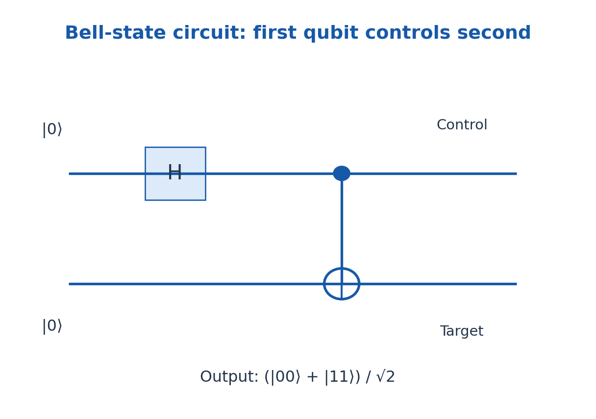
Prepare |00⟩, apply H to the first qubit and then CNOT with that qubit as control. The output is (|00⟩ + |11⟩)/√2, a Bell state. It cannot be written as a single product of two pure one-qubit states. Computational-basis outcomes are perfectly correlated, with probabilities one half for 00 and 11.
Entanglement is a property of the joint state, not merely two objects having similar local values. A classical mixture of 00 and 11 has the same computational-basis correlation but differs in other measurements. Entanglement cannot by itself send a chosen message faster than light; local outcomes remain probabilistic.
Worked Problem 3.6: Bell-State Preparation
Problem: Start in |00⟩, apply H on the first qubit and CNOT with first control and second target. Find nonzero measurement probabilities.
Method: Expand the superposition before using the CNOT truth table.
Calculation: After H: (|00⟩ + |10⟩)/√2; CNOT sends the second term to |11⟩.
Answer: Output (|00⟩ + |11⟩)/√2; P(00) = P(11) = 1/2.
Check: Control and target ordering is part of the question; outcomes 01 and 10 have probability zero.
Worked Problem 3.7: Product-State Expansion
Problem: Expand |+⟩⊗(√3|0⟩ + |1⟩)/2 and find P(10).
Method: Tensor-product coefficients follow ordered basis 00, 01, 10, 11.
Calculation: Coefficients are √3/(2√2), 1/(2√2), √3/(2√2), 1/(2√2).
Answer: P(10) = 3/8; the total of all four probabilities is one.
Check: This state is separable by its given construction; multiple nonzero amplitudes alone do not imply entanglement.
5. Decoherence, Relaxation and Practical Errors
A qubit interacting with uncontrolled surroundings can lose coherence in the selected description. Decoherence suppresses interference when information about the system becomes correlated with an environment that is ignored. It is not simply an incorrect arithmetic operation or an instrument displaying a blurry result.
Energy relaxation is often characterised by T1, while transverse phase coherence is characterised by T2 under a specified model. Pure dephasing has time Tφ. In a common Markovian model, 1/T2 = 1/(2T1) + 1/Tφ, so T2 ≤ 2T1. These relations are model dependent and differ from an arbitrary device-error percentage.
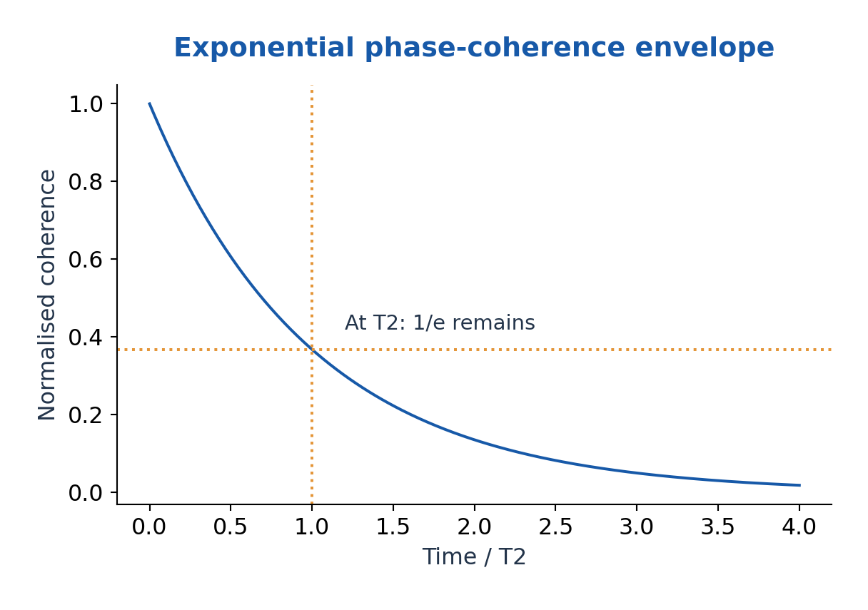
Gate errors, readout errors, leakage outside the chosen two levels and environmental drift can all affect a circuit. More gates or longer duration generally creates more opportunities for error. A simple decay exp(-t/T2) estimates coherence in the stated exponential model, not the universal success probability of every algorithm.
Isolation, low-noise control, calibration, echo sequences and quantum error correction address different error mechanisms. Error correction encodes logical information across physical systems and uses syndrome information; it does not make an unrestricted copy of an unknown quantum state. The no-cloning theorem forbids such a universal perfect copier.
Worked Problem 3.8: Coherence Envelope
Problem: In an exponential model T2 = 40 microseconds. Find the coherence fraction after 20 microseconds.
Method: Fraction = exp(-t/T2).
Calculation: The ratio t/T2 = 0.5; no unit conversion is needed if both times use the same unit.
Answer: Coherence fraction = 0.60653.
Check: This is the model coherence envelope, not a universal circuit-success probability.
Worked Problem 3.9: Relaxation and Pure Dephasing
Problem: Use T1 = 50 microseconds and Tφ = 100 microseconds in 1/T2 = 1/(2T1) + 1/Tφ. Find T2.
Method: Add rates, then invert.
Calculation: 1/T2 = 1/100 + 1/100 = 0.0200 per microsecond.
Answer: T2 = 50.0 microseconds; T2 ≤ 2T1 is satisfied.
Check: Adding the times themselves would give the wrong physical model.
6. Solid-State and Photonic Qubit Realisations
Solid-state qubits encode two selected levels in fabricated material systems. Superconducting circuits use engineered circuit quantum states controlled by microwave fields, normally at cryogenic temperatures. Spin qubits can use electron or nuclear spin states in semiconductors or defects, with magnetic, microwave or electrical control depending on the design.
A quantum dot confines carriers in a small region. Its orbital or spin structure may supply the relevant states, but any small dot is not automatically a useful qubit. Initialisation, coherence, selective control, coupling to other qubits and reliable readout are all needed.
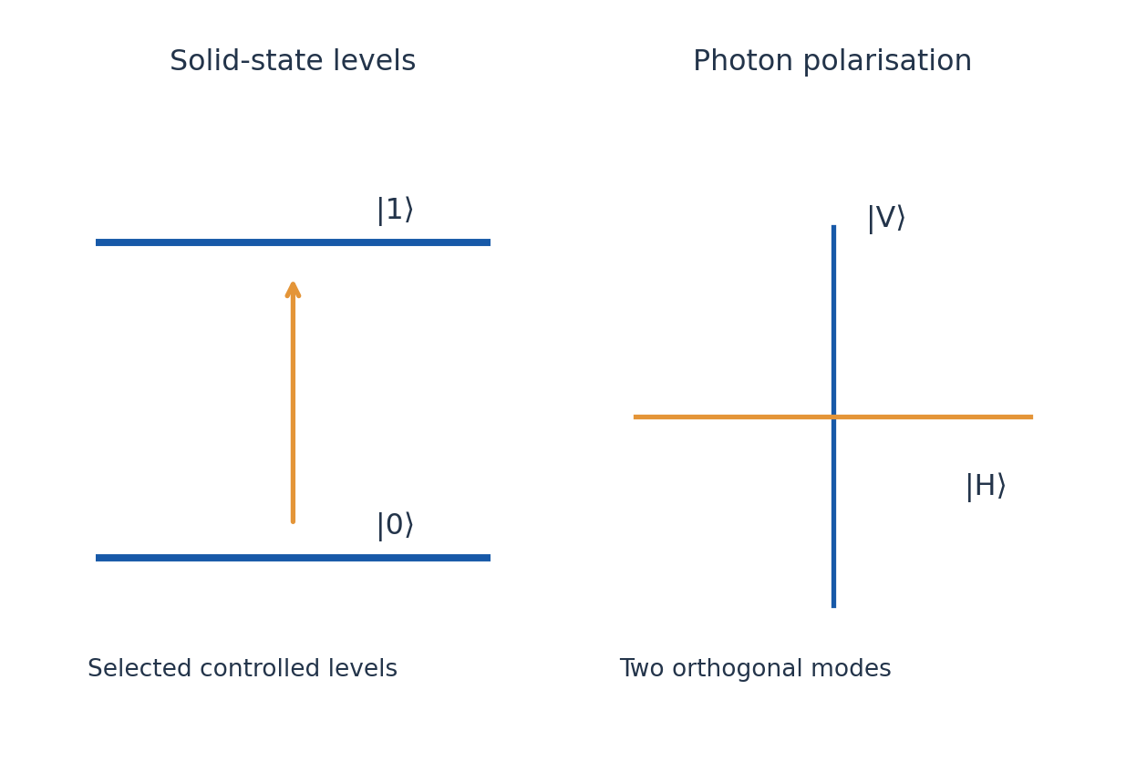
Photonic qubits may encode information in two polarisation modes, two paths or two time bins. Single photons are useful carriers for optical communication. Loss destroys a transmitted photon’s availability, while imperfect sources, detectors and interferometer stability affect observed results. Polarisation encoding and path encoding require different optical components.
Compare implementations using encoding, control, coupling, measurement and dominant practical limitations. Do not confuse a platform’s physical qubit count with its number of protected logical qubits. This unit explains the principles without treating one hardware platform as a universal solution.
7. Quantum Communication, Cryptography and QKD
Quantum communication uses controlled quantum states to distribute information resources or cryptographic keys. Quantum cryptography is distinct from running ordinary encryption on a faster processor. Quantum key distribution, or QKD, establishes correlated secret-key material under an explicit security model; the key is later used in a classical cryptographic application.
A QKD link needs a quantum channel and an authenticated classical channel. The classical discussion need not be secret, but authenticity prevents an adversary from impersonating the users. QKD does not remove the need for endpoint security, authentication and careful treatment of imperfect hardware.
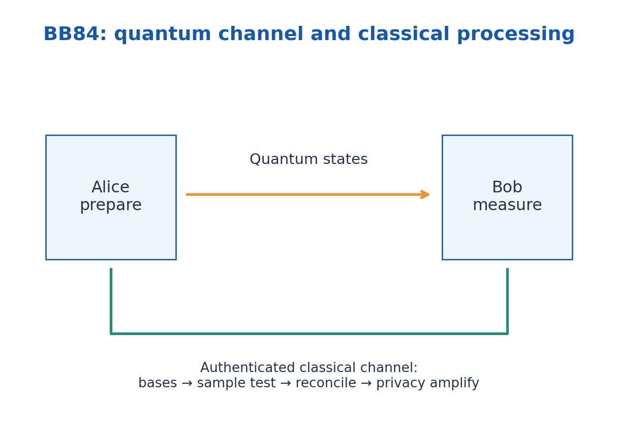
The BB84 prepare-and-measure scheme uses two noncommuting bases. Alice randomly selects a bit and a basis, sending one of |0⟩, |1⟩, |+⟩, |-⟩. Bob randomly chooses one of the two measurement bases. Matching choices recover the ideal sent bit; mismatched choices yield random outcomes.
After transmission, the users reveal basis choices, keep matching-basis events, estimate error using a sacrificed sample, reconcile discrepancies and apply privacy amplification according to the protocol and security analysis. BB84 need not use pre-shared entangled pairs. It distributes a key, not the message itself.
8. BB84 Error Checks and the No-Cloning Connection
In a simple intercept-resend attack Eve measures every travelling qubit in a randomly chosen BB84 basis and resends the corresponding state. On the sifted events where Alice and Bob used the same basis, Eve chose the wrong basis half the time. In those cases Bob’s bit is wrong with probability one half. The induced ideal sifted-key error rate is therefore one quarter.
This 25% calculation belongs to that attack model. It is not a universal error threshold for all QKD implementations. Loss, background counts, imperfect sources and sophisticated attacks require a fuller security analysis. A low measured sample error is evidence used in the protocol, not a guarantee that an unanalysed device is secure.
No cloning explains why Eve cannot in general make a perfect copy of an unknown member of nonorthogonal quantum states while leaving the original unchanged. If a unitary copied both |a⟩ and |b⟩, preserving inner products would require ⟨a|b⟩ = ⟨a|b⟩², which fails for overlap strictly between zero and one.
In an exam answer distinguish physical disturbance, public basis announcement, sampling cost and final key processing. Raw transmitted bits, sifted bits and final secret bits are different counts. For ideal independent random basis choices, about half the detected events survive basis sifting before further reductions.
Worked Problem 3.10: BB84 Sifting and Intercept-Resend
Problem: There are 10000 ideal detected events with independent random bases. Estimate sifted events and wrong sifted bits under a full random-basis intercept-resend attack.
Method: Basis match probability 1/2; conditional attack error probability 1/4.
Calculation: Expected sifted count = 10000/2 = 5000; wrong sifted bits = 5000/4.
Answer: About 5000 sifted events and 1250 wrong sifted bits before further processing.
Check: These are expectations for this attack model, not the final secret-key length or a universal security threshold.
9. B. Basic Electric and Magnetic Laws – EE and ECE
Electric charge produces electric fields and moving charge contributes to magnetic fields. The Lorentz force on a particle is F = q(E + v × B). Electric force can do work through the component along velocity; magnetic force is perpendicular to velocity and changes direction rather than kinetic energy for a point charge acted on by that force alone.
Gauss’ electric law relates electric flux to enclosed charge. In vacuum, integral E·dA = Qenc/ε0 for a closed surface. Symmetry can make it a calculation tool, but the law remains valid without symmetry. Gauss’ magnetic law gives zero net magnetic flux through a closed surface: ideal isolated magnetic monopoles are not included in this classical theory.
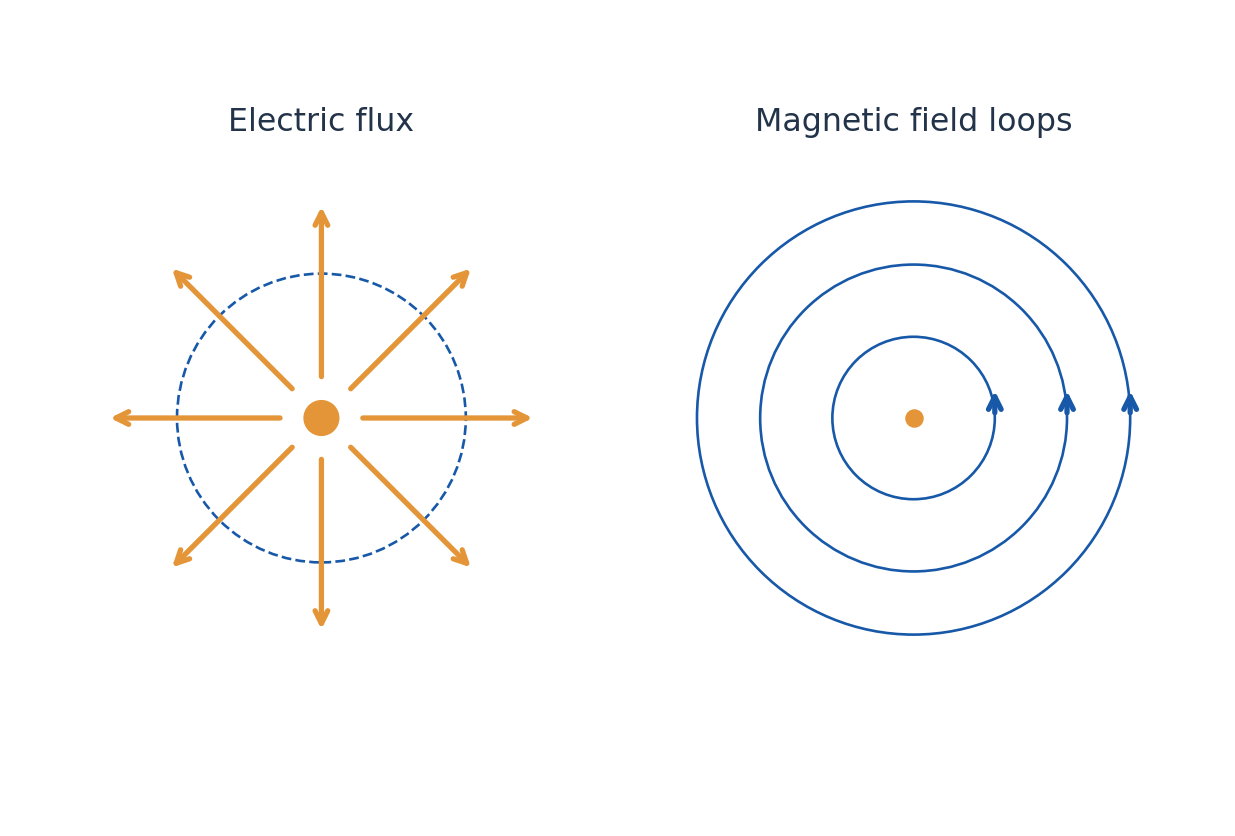
Faraday induction says a changing magnetic flux generates a circulating electric field: integral E·dl = -dΦB/dt for a fixed loop. The minus sign expresses the orientation and Lenz-law opposition. In magnetostatics, Ampere circulation relates H to enclosed free current; changing fields require Maxwell’s additional displacement-current term.
Macroscopic fields use D = ε0E + P and B = μ0(H + M). In a simple linear isotropic material, D = εE, B = μH and J = σE. These are constitutive assumptions, not extra universal Maxwell equations. Distinguish free charge/current from the material response included in P and M.
Worked Problem 3.11: Lorentz-Force Components
Problem: A charge +2.0 microC moves at 3000 m/s along +x. E = 100 xhat V/m and B = 0.20 zhat T. Find force components.
Method: v × B is along -y; F = qE + q(v × B).
Calculation: Fx = 2 × 10^-6 × 100; Fy = -(2 × 10^-6)(3000)(0.20).
Answer: Fx = +2.00 × 10^-4 N; Fy = -1.20 × 10^-3 N; Fz = 0.
Check: For a negative charge both components would reverse. The magnetic part is perpendicular to velocity.
Worked Problem 3.12: Electric Flux and Enclosed Charge
Problem: A closed surface in vacuum encloses +3.0 nC. Find net outward electric flux.
Method: Electric flux = Qenc/ε0.
Calculation: Qenc = 3.0 × 10^-9 C; use ε0 in SI.
Answer: Net electric flux = 338.82 N m²/C.
Check: Shape and size do not change the net enclosed-charge flux; they can change the local field distribution.
10. Continuity Equation and Displacement Current
Charge conservation states that outward current from a closed volume reduces its stored charge: integral J·dA = -dQinside/dt. In local form, ∇·J + ∂ρ/∂t = 0. A positive divergence means more charge leaves than enters locally. In steady state the time derivative vanishes, so ∇·J = 0.
A charging capacitor exposes the limitation of the uncorrected Ampere law. A surface cutting the wire intercepts conduction current; a surface bulging between the plates intercepts no ideal conduction current. Both share the same bounding loop, so a consistent circulation law needs the changing electric-displacement flux.
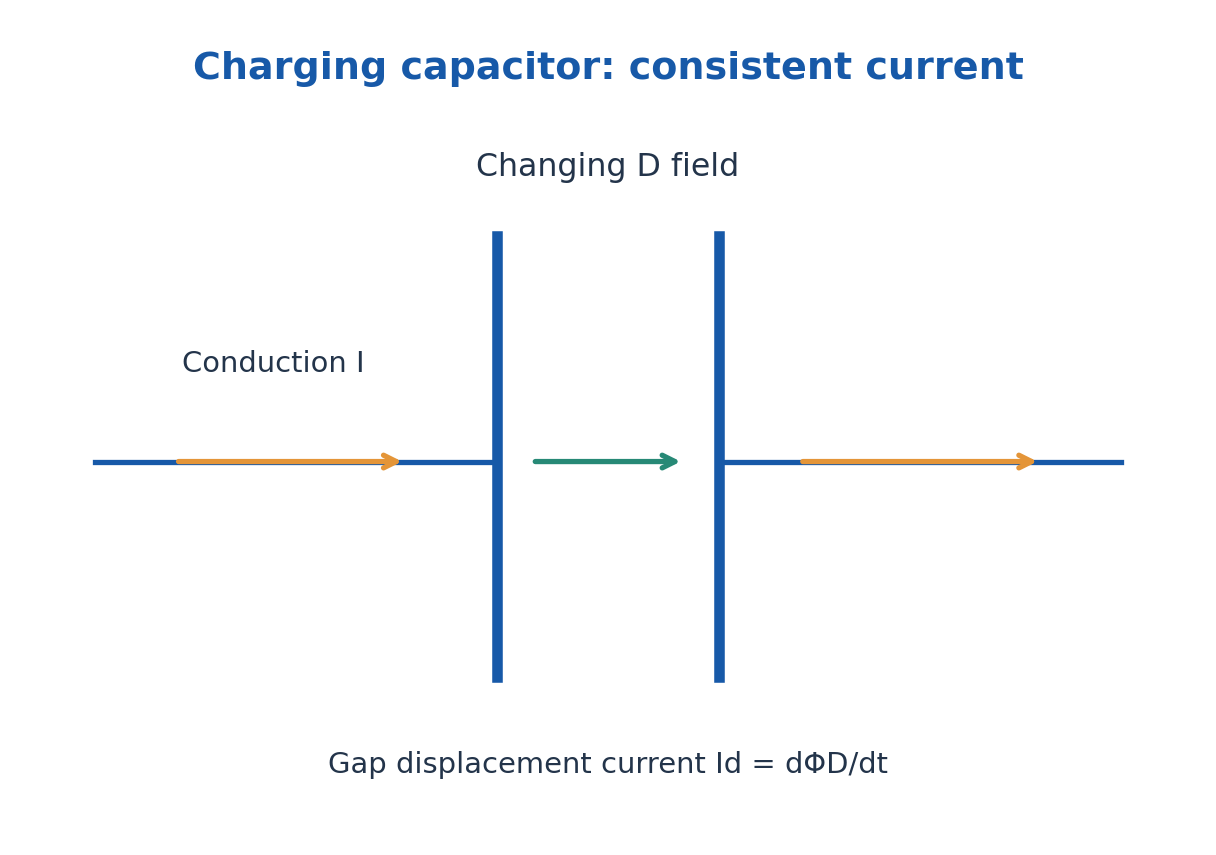
Displacement current density is Jd = ∂D/∂t; total displacement current is d(integral D·dA)/dt. It is not literal electron flow across the dielectric gap. In an ideal parallel-plate capacitor, D = Q/A, so integrated displacement current equals dQ/dt, the current in the connecting wire.
Taking divergence of ∇×H = Jfree + ∂D/∂t and using ∇·D = ρfree gives the free-charge continuity equation. Maxwell’s correction therefore preserves charge conservation as well as supporting electromagnetic waves.
Worked Problem 3.13: Charge Conservation in a Volume
Problem: Outward current through a closed boundary is 4.0 mA and no other transfer is present. Find charge change in 3.0 ms.
Method: dQ/dt = -Iout.
Calculation: ΔQ = -(4.0 × 10^-3)(3.0 × 10^-3).
Answer: ΔQ = -12.0 microC.
Check: Outward positive current reduces stored positive charge.
Worked Problem 3.14: Capacitor Displacement Current
Problem: A vacuum parallel-plate capacitor has area 0.0100 m². Its uniform field rises at 2.0 × 10^8 V/(m s). Find displacement current.
Method: Id = ε0 A dE/dt.
Calculation: Substitute area and the time derivative, not the field magnitude.
Answer: Id = 1.7708 × 10^-5 A.
Check: The same ideal charging current flows in the wire; no conduction across the vacuum gap is required.
11. Maxwell Equations: Integral and Differential Forms
In a macroscopic description, the four equations are ∇·D = ρfree; ∇·B = 0; ∇×E = -∂B/∂t; and ∇×H = Jfree + ∂D/∂t. Divergence describes local net flux per volume; curl describes local circulation. The fields are vector quantities and signs depend on consistently chosen orientations.
The corresponding integral forms are: closed-surface integral D·dA = Qfree; closed-surface integral B·dA = 0; closed-loop integral E·dl = -d(integral B·dA)/dt; and closed-loop integral H·dl = Ifree + d(integral D·dA)/dt. The loop direction and surface normal follow the right-hand rule.
The divergence theorem relates closed-surface flux to a volume integral of divergence. Stokes’ theorem relates loop circulation to surface integral of curl. These connect the two forms when fields and boundaries satisfy the required regularity conditions. Integral laws are especially helpful at interfaces or with symmetry.
In vacuum substitute D = ε0E and B = μ0H. In a stationary uniform linear conductor also use J = σE. Charge-free does not mean field-free, and a time-varying electric field can exist without conduction current. Always state which terms have been set to zero and why.
| Equation | Physical Statement |
|---|---|
| Gauss electric | Free charge sources electric-displacement flux |
| Gauss magnetic | No net closed-surface magnetic flux |
| Faraday | Changing magnetic flux drives electric circulation |
| Ampere-Maxwell | Conduction and displacement drive magnetic circulation |
12. Plane Electromagnetic Waves in Vacuum
In source-free vacuum, taking curl of Faraday’s law and using the Ampere-Maxwell law gives ∇²E = μ0ε0 ∂²E/∂t²; similarly for B. The vector identity ∇×(∇×E) = ∇(∇·E) – ∇²E and zero vacuum charge density are used explicitly.
The wave speed is c = 1/√(μ0ε0). A plane wave travelling in +z can have E = E0 cos(kz – ωt) xhat and B = (E0/c)cos(kz – ωt) yhat, with k = ω/c. E, B and propagation are mutually perpendicular and form the correct right-handed orientation.
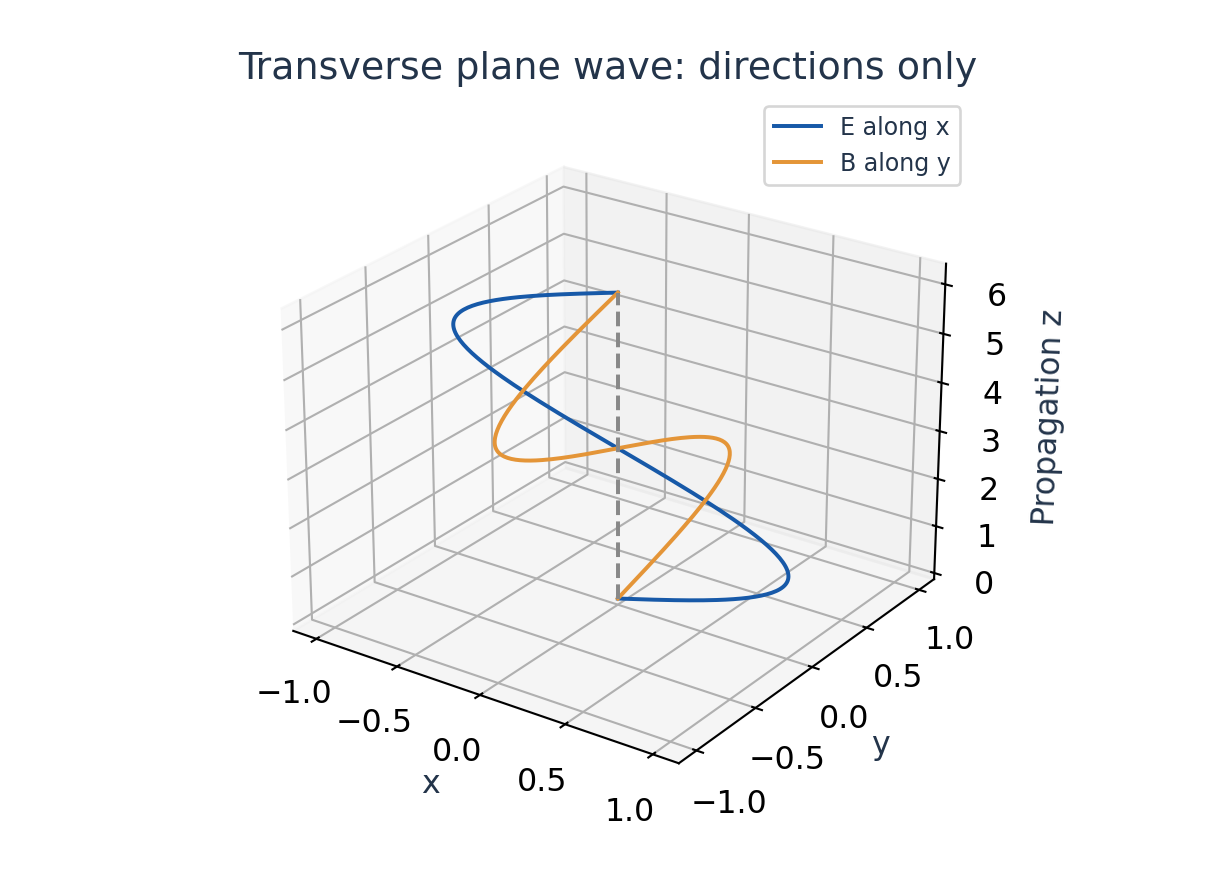
In vacuum E and B are in phase. Their amplitudes satisfy E0/B0 = c, while E0/H0 = Z0 = √(μ0/ε0), about 376.73 ohm. Do not substitute H for B without the factor μ0. Frequency f, wavelength λ and angular quantities obey c = fλ and ω = 2πf.
A field depending on position and time does not automatically satisfy Maxwell equations. Its direction, phase, amplitude relation and dispersion must be consistent. The wave transports energy; the field magnitudes do not describe a material medium oscillating through empty space.
Worked Problem 3.15: Wave Frequency, Magnetic Field and H
Problem: A vacuum plane wave has f = 100 MHz and peak E0 = 12.0 V/m. Find λ, B0 and H0.
Method: λ = c/f; B0 = E0/c; H0 = E0/Z0.
Calculation: Z0 = √(μ0/ε0); convert MHz to 10^6 Hz.
Answer: λ = 2.99792 m; B0 = 4.0028 × 10^-8 T; H0 = 0.031853 A/m.
Check: B and H have different units. Peak quantities remain peak in these amplitude relations.
Worked Problem 3.16: Wave Direction
Problem: A plane vacuum wave has E along +y and B along -x at an instant. Determine propagation direction.
Method: Energy flow is along E × H, and H is parallel to B in vacuum.
Calculation: yhat × (-xhat) = +zhat.
Answer: Propagation and energy flow are along +z.
Check: Reversing both E and B together would leave their cross-product direction unchanged.
13. Electromagnetic Waves in a Conducting Medium
For a homogeneous linear isotropic conductor with constant μ, ε and σ, a source-free bulk transverse field obeys ∇²E = με ∂²E/∂t² + μσ ∂E/∂t. The first time-derivative term represents conduction loss. The same form applies to H under the corresponding uniform-medium assumptions.
Using the convention E ∝ exp(-αz)cos(ωt – βz), the propagation constant is γ = α + iβ, with γ² = iωμ(σ + iωε). Both attenuation α and phase constant β are positive for the passive +z wave. The exact values follow from α = ω√(με/2)√[√(1 + (σ/ωε)²) – 1] and β with the minus one replaced by plus one.
The intrinsic impedance is η = √[iωμ/(σ + iωε)]. It is generally complex, so E and H are not generally in phase. In a good conductor σ is much greater than ωε; α ≈ β ≈ √(ωμσ/2) and η ≈ (1 + i)√(ωμ/(2σ)) with the stated time convention.
In a lossless dielectric σ = 0, attenuation vanishes and β = ω√(με). A good-conductor approximation must be checked at the stated frequency and material parameters. Avoid claiming that every conductor has zero interior time-varying field; finite conductivity allows penetration with decay.
14. Poynting Vector and Electromagnetic Energy Conservation
The instantaneous Poynting vector is S = E × H, in W/m². Its direction indicates electromagnetic energy flow. For a fixed region, the outward surface integral gives net power leaving that region. A local negative divergence means energy is entering or accumulating, depending on work and storage.
For linear nondispersive media with time-independent ε and μ, field energy density is u = (E·D + B·H)/2. Combining Maxwell curl equations with ∇·(E×H) = H·(∇×E) – E·(∇×H) gives ∂u/∂t + ∇·S + J·E = 0. The last term is power delivered to charges per volume.
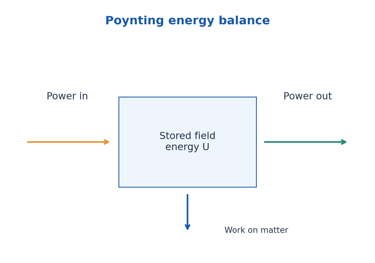
For an Ohmic conductor J·E = σE² ≥ 0, representing dissipative heating. In a general system the term is field-to-matter work and should not always be labelled pure heat. Dispersive or nonlinear material energy requires additional care beyond the simple u expression.
For a sinusoidal vacuum wave with peak electric amplitude E0, average intensity is E0²/(2Z0) = ε0cE0²/2. With rms fields it is Erms²/Z0. Complex phasors with peak amplitudes give average S = Re(E × H*)/2. State peak or rms before inserting a factor of two.
Worked Problem 3.17: Intensity and Beam Power
Problem: A vacuum wave has peak E0 = 20.0 V/m and illuminates a perpendicular area 0.0200 m² uniformly. Find average power.
Method: Iavg = E0²/(2Z0); Pavg = Iavg A.
Calculation: Use peak amplitude, hence the factor one half.
Answer: Iavg = 0.53088 W/m²; Pavg = 0.01062 W.
Check: If 20.0 V/m were rms instead, the predicted average power would double.
Worked Problem 3.18: Poynting Energy Budget
Problem: A region receives 12 W net electromagnetic power. Fields transfer 7 W to matter. Find the stored-field energy rate.
Method: Input power = dUfield/dt + power to matter.
Calculation: dUfield/dt = 12 – 7.
Answer: Field energy increases at 5.0 J/s.
Check: Net outward flux would be -12 W; the sign convention must be declared.
15. Skin Depth and Frequency-Dependent Penetration
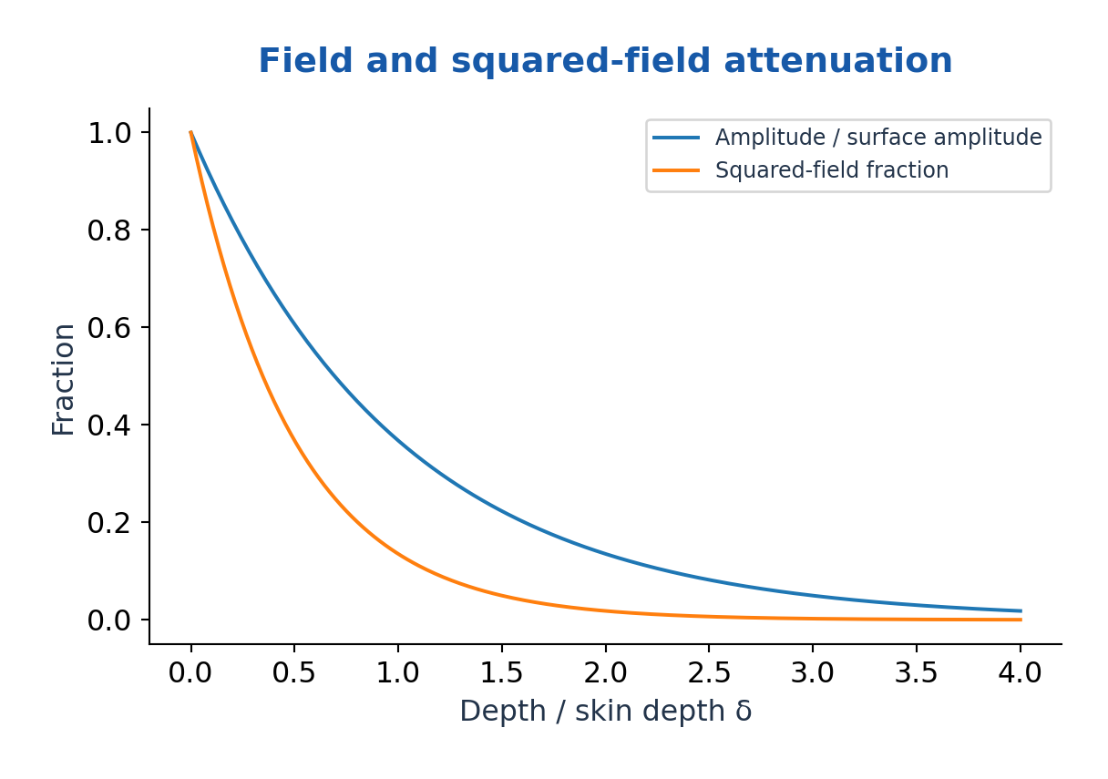
Skin depth δ is the distance at which field amplitude falls to 1/e of its surface value in the simple exponential model: δ = 1/α. In a good conductor δ ≈ √[2/(ωμσ)] = 1/√(πfμσ). It decreases with the square root of frequency, conductivity or permeability when the approximation remains valid.
Because intensity is proportional to squared amplitude in the corresponding uniform wave model, it decays as exp(-2z/δ), not exp(-z/δ). At one skin depth amplitude is about 36.8% but the associated squared-field factor is about 13.5%.
Skin effect concentrates alternating current toward the surface of a sufficiently thick conductor. This can increase AC resistance and affects shielding and induction heating. A thin wire or film requires consideration of its dimensions relative to δ; the infinite half-space picture cannot be applied blindly.
Permeability can depend on frequency, field strength and material state, especially for magnetic materials. Use the supplied value and note the assumption. Skin depth is a penetration length, not the same thing as electromagnetic wavelength in vacuum.
Worked Problem 3.19: Copper Skin Depth
Problem: For a good conductor with σ = 5.8 × 10^7 S/m and μ = μ0 at 1.00 MHz, estimate δ.
Method: δ = √[2/(ωμσ)].
Calculation: ω = 2π × 10^6 rad/s; check σ greatly exceeds ωε0.
Answer: δ = 6.6085 × 10^-5 m = 66.0855 micrometres.
Check: The estimate assumes a uniform nonmagnetic good conductor and a thickness large relative to δ.
Worked Problem 3.20: Amplitude and Power Penetration
Problem: At depth z = 2δ in the same exponential field model, find amplitude fraction and squared-field fraction.
Method: Amplitude ratio exp(-z/δ); squared ratio exp(-2z/δ).
Calculation: Set z/δ = 2.
Answer: Amplitude = 0.13534; squared-field factor = 0.01832.
Check: Skin depth is defined for field amplitude; using the same decay for power loses a factor two in the exponent.
16. C. Dielectric Fields, Polarisation and Susceptibility – BT
A dielectric responds to an applied electric field mainly through bound-charge displacement and orientation rather than large steady free-current flow. Polarisation P is electric dipole moment per unit volume, in C/m². The macroscopic displacement is D = ε0E + P and Gauss’ law uses ∇·D = ρfree.
For a linear isotropic dielectric, P = ε0χe E, ε = ε0(1 + χe) and relative permittivity εr = 1 + χe. Susceptibility is dimensionless. These simple scalar relations do not describe every anisotropic, nonlinear or frequency-dependent material.
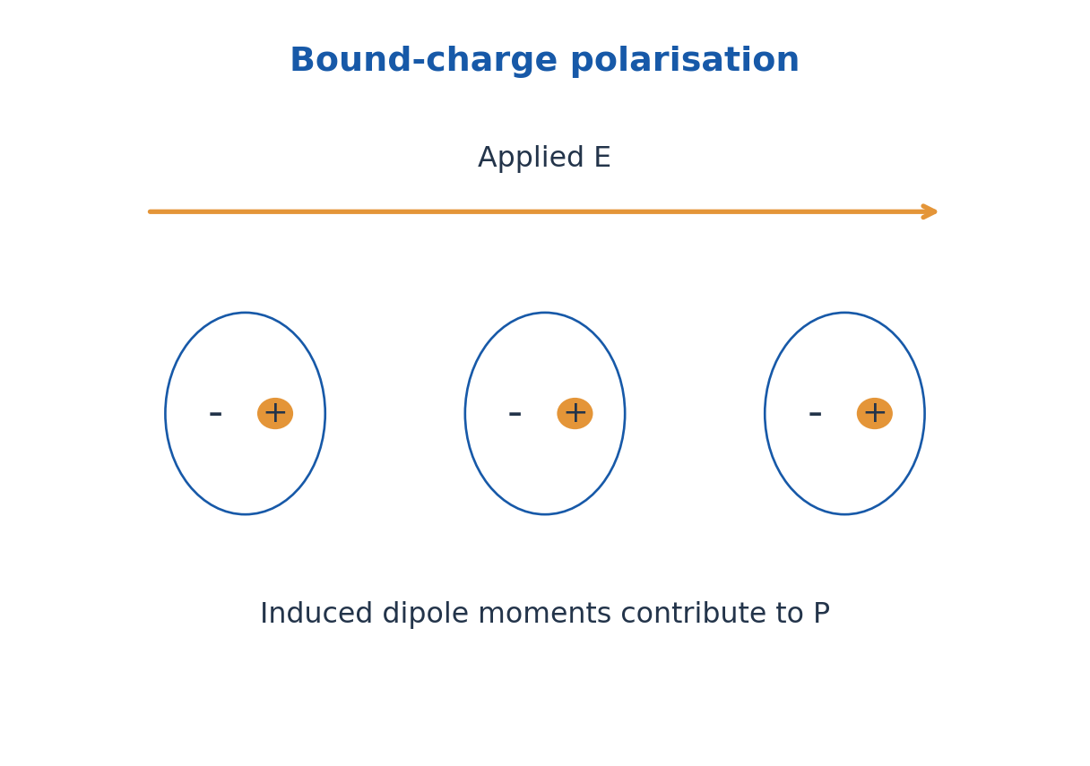
A parallel-plate capacitor of area A and separation d has C = εA/d when fringe effects are negligible. Filling the gap with a suitable dielectric increases capacitance. At fixed voltage its stored energy rises because the source supplies charge; for a disconnected capacitor with fixed charge the energy falls. State the electrical constraint.
Useful properties include permittivity, dielectric strength, loss and stability. A high dielectric constant does not automatically mean low loss or high breakdown strength. Capacitors, insulation and sensing applications require different compromises.
Worked Problem 3.21: Dielectric Vectors
Problem: A linear isotropic dielectric has εr = 4.0 and E = 2.0 × 10^5 V/m. Find χe, P and D magnitudes.
Method: χe = εr – 1; P = ε0χeE; D = ε0εrE.
Calculation: χe = 3; multiply ε0E by three or four respectively.
Answer: χe = 3.0; P = 5.3125 × 10^-6 C/m²; D = 7.0834 × 10^-6 C/m².
Check: D – P = ε0E, a direct consistency check.
Worked Problem 3.22: Dielectric Capacitance and Energy
Problem: A capacitor has εr = 5.0, A = 0.0200 m², d = 1.00 mm and voltage 100 V. Find C and stored energy, neglecting fringes.
Method: C = εA/d; U = CV²/2.
Calculation: ε = 5ε0; d = 10^-3 m.
Answer: C = 0.88542 nF; U = 4.4271 × 10^-6 J.
Check: This is a fixed-voltage statement; a disconnected fixed-charge insertion is a different energy problem.
17. Polarisation Mechanisms and Dielectric Applications
Electronic polarisation shifts the electron cloud relative to the nucleus. Ionic polarisation displaces positive and negative sublattices in ionic materials. Orientation polarisation aligns permanent dipoles against thermal disorder. Space-charge or interfacial polarisation results from charge accumulation at interfaces or in heterogeneous structures.
The mechanisms respond on different timescales. As field frequency rises, slower mechanisms can no longer follow the oscillation effectively, changing the real permittivity and dissipative loss. Orientation contributions generally weaken with increasing temperature in simple dilute-dipole models because thermal agitation opposes alignment.
If an individual induced dipole is p = αaE and interactions are neglected, P ≈ NαaE. The molecular polarizability αa has units C m²/V; it is not the same as dimensionless bulk susceptibility. Dense materials require a local-field model before connecting the two accurately.
Dielectric materials are used in capacitors, electrical insulation, substrates and sensors. In biotechnology, dielectric measurements can probe hydration and material response, but observed signals depend on geometry, frequency and conduction as well as polarisation. Select an operating frequency and calibration rather than assigning a specimen one universal dielectric value.
Worked Problem 3.23: Induced-Dipole Estimate
Problem: Ignore local-field corrections. N = 2.0 × 10^28 m^-3, atomic polarizability αa = 1.0 × 10^-40 C m²/V and E = 10^5 V/m. Find P and approximate χe.
Method: P = NαaE; χe = Nαa/ε0.
Calculation: First multiply N and αa; χe must be dimensionless.
Answer: P = 2.00 × 10^-7 C/m²; χe ≈ 0.22588.
Check: The estimate is explicitly a dilute/local-field-neglect model, not an exact dense-material identity.
18. Magnetic Susceptibility and Material Classes
Magnetisation M is magnetic dipole moment per volume, in A/m. The macroscopic relation is B = μ0(H + M). In a weak linear isotropic response, M = χmH and μr = 1 + χm. Magnetic susceptibility χm is dimensionless; permeability has different units.
Diamagnets have a small negative susceptibility in the simple static description and tend to oppose applied field. Paramagnets have small positive susceptibility associated with permanent moments tending to align. Ferromagnets show cooperative ordering, domains, strong nonlinear response and hysteresis below the relevant transition temperature.
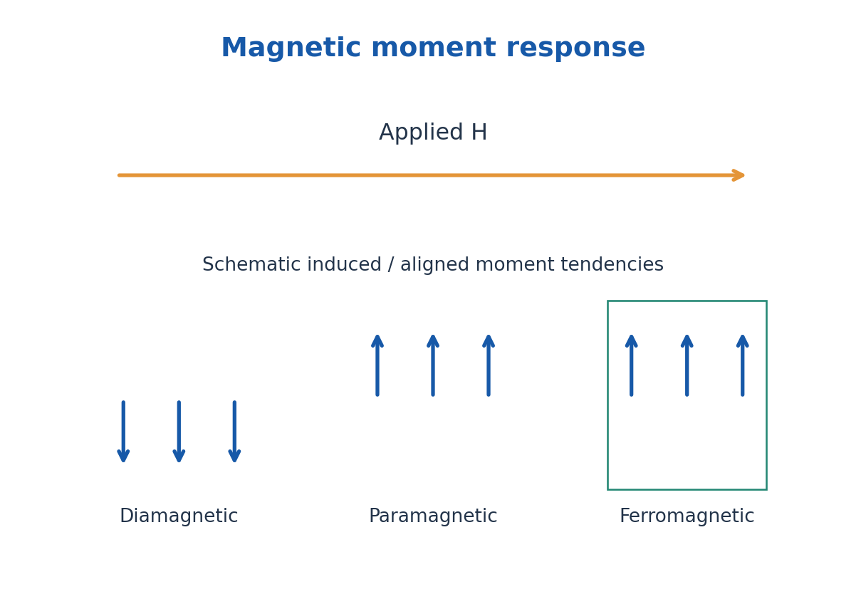
In a simple paramagnetic regime, Curie’s law gives χm = C/T with absolute temperature T. It is not a general law for every temperature, field or material. Ferromagnetic ordering disappears above a Curie temperature, where an appropriate paramagnetic description becomes necessary.
Domain-wall movement and moment rotation explain much of ferromagnetic magnetisation. A domain is a region of aligned moments, not a separate lump of electric charge. Soft magnetic materials are useful when magnetisation must reverse with low loss; hard magnetic materials retain strong magnetisation for permanent-magnet applications.
| Type | Ideal Weak-Field Trend |
|---|---|
| Diamagnetic | Small χm < 0; induced opposition |
| Paramagnetic | Small χm > 0; thermal competition |
| Ferromagnetic | Domains, nonlinearity and hysteresis |
Worked Problem 3.24: Magnetisation and Flux Density
Problem: A weak linear material has χm = 2.0 × 10^-3 and H = 1000 A/m. Find M and B.
Method: M = χmH; B = μ0(H + M).
Calculation: M = 2.0 A/m; total H + M = 1002 A/m.
Answer: M = 2.0 A/m; B = 0.00125915 T.
Check: Positive susceptibility here indicates a small paramagnetic-like response, not ferromagnetic saturation.
19. Hysteresis, Coercivity, Remanence and Losses
When a ferromagnet is driven through a cycle, its response depends on previous magnetisation. In a B-H loop, remanent flux density Br is the remaining B when H returns to zero after magnetisation. Coercive field Hc is the reverse H needed to bring B to zero on the specified loop.
Saturation describes the approach to maximum alignment under strong field. Remanence, coercivity and saturation are distinct. A narrow loop generally indicates lower hysteresis loss and easier reversal, while a wide loop indicates greater resistance to demagnetisation. Measurement definitions and material conditions should be stated.
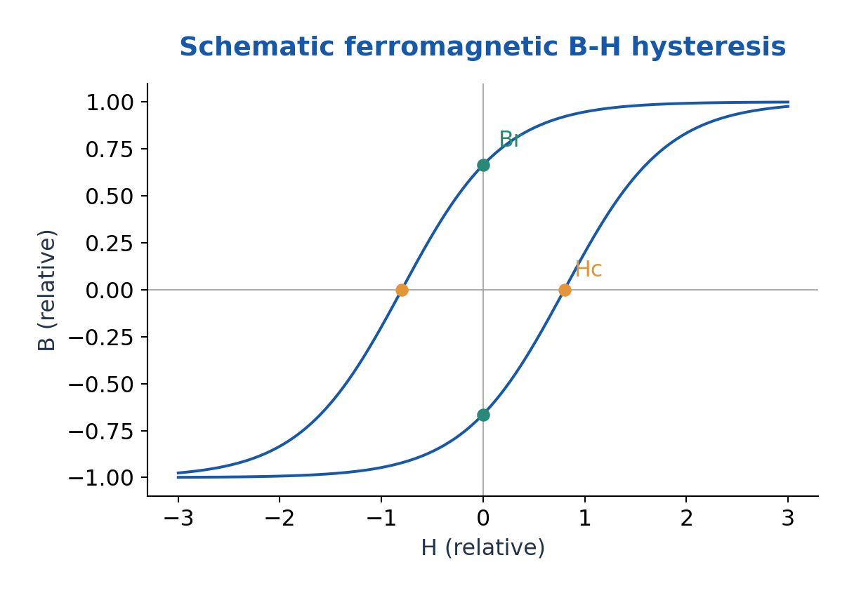
For quasistatic cyclic operation, hysteresis energy dissipated per volume per cycle is the magnitude of the loop area ∮H dB, in J/m³. Multiply by frequency and core volume to estimate hysteresis power under the stated assumption that loop area is unchanged. Eddy-current and other dynamic losses are additional.
Applications include transformer and motor cores, permanent magnets and magnetic recording. Reducing hysteresis loss is valuable for frequently reversing cores; high coercivity is valuable for magnets resisting accidental demagnetisation. A permanent magnet and an efficient AC core therefore need different properties.
Worked Problem 3.25: Hysteresis Power
Problem: A measured loop area is 120 J/m³ per cycle. Core volume is 4.0 × 10^-4 m³ and frequency is 50 Hz. Estimate hysteresis power with fixed loop area.
Method: P = loop area × volume × frequency.
Calculation: P = 120 × 4.0 × 10^-4 × 50.
Answer: P = 2.40 W.
Check: Eddy-current and other losses must be added separately; the loop area can change with operating conditions.
20. D. Bands, Conductors and Semiconductors – TX
In a crystal, interacting atomic states form energy bands separated by forbidden gaps. Electrical conduction depends on allowed states, their occupation and carrier mobility. A partially filled band or suitable band overlap supports metallic conduction, while a full band alone cannot carry ordinary small-field net current in the ideal picture.
A semiconductor has accessible thermal or optical excitation across a gap from valence to conduction states. Excitation creates an electron and a valence hole. An insulator has a much less accessible excitation gap under ordinary operating conditions. There is no one temperature-independent numerical gap boundary that perfectly separates the categories.
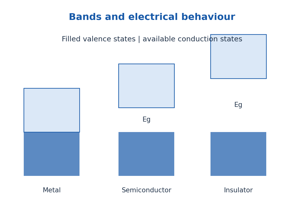
Intrinsic semiconductors have equilibrium n = p. Doping supplies donors or acceptors that shift the majority-carrier balance. Conductivity is σ = e(nμn + pμp), and resistivity is its reciprocal. For metals, temperature commonly increases scattering; for intrinsic semiconductors, thermally activated carriers can dominate the temperature response.
Textile electronics can combine conductors, semiconductors and insulators for interconnects, sensing and protection. Mechanical flexibility, humidity, adhesion and contact resistance also matter. This band-theory overview is the TX Unit III requirement; the full solids-statistics treatment occurs in other branches at a different unit number.
Worked Problem 3.26: Two-Carrier Conductivity
Problem: A sample has n = 2.0 × 10^20 and p = 1.0 × 10^18 m^-3, with μn = 0.10 and μp = 0.050 m²/(V s). Find σ.
Method: σ = e(nμn + pμp).
Calculation: nμn = 2.0 × 10^19 and pμp = 5.0 × 10^16 in matching SI units.
Answer: σ = 3.21236 S/m.
Check: Conventional electron and hole current contributions add; their charges do not cause cancellation in this conductivity formula.
21. Dielectrics, Piezoelectricity and Ferroelectricity – TX
TX also requires dielectric materials: use D = ε0E + P to distinguish applied field, bound-charge response and free-charge flux. For a linear isotropic material P = ε0χeE and εr = 1 + χe. A dielectric stores field energy but real materials can also have conduction and polarisation loss.
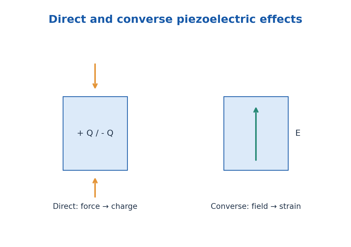
The direct piezoelectric effect is electric polarisation produced by suitable mechanical stress. The converse effect is mechanical strain produced by an applied field. It requires an appropriate non-centrosymmetric crystal symmetry; not every dielectric is piezoelectric. In a simplified one-dimensional sensor model, charge Q = dF with d in C/N.
Ferroelectric materials possess a spontaneous polarisation that can be switched by an applied electric field. Their P-E response can exhibit hysteresis, with remanent polarisation and coercive field. Ferroelectricity is not a requirement for iron atoms, and a permanent electric dipole alone does not prove switchable ferroelectric order.
Ferroelectric materials are piezoelectric in their polar phase, but many piezoelectrics are not ferroelectric. Applications include pressure and vibration sensors, actuators, ultrasonic transducers, capacitors and non-volatile memory. In a wearable textile, packaging must transmit the intended stress without shorting or damaging the active layer.
Worked Problem 3.27: Piezoelectric Sensor Charge
Problem: An ideal one-dimensional piezoelectric element has d = 250 pC/N and load 40 N. Find generated charge and voltage if its capacitance is 2.0 nF.
Method: Q = dF; open-circuit ideal voltage V = Q/C.
Calculation: Q = 250 × 10^-12 × 40 = 10^-8 C.
Answer: Q = 10.0 nC; V = 5.0 V.
Check: This simplified estimate neglects leakage, mechanical boundary effects and the measuring instrument load.
22. E. Thermal Physics: Laws and First-Law Signs – ME and TX
Temperature describes thermal equilibrium; internal energy is a state function; heat and work are transfers across a system boundary. The zeroth law supports temperature measurement. A thermometer should reach equilibrium without significantly disturbing the sample.
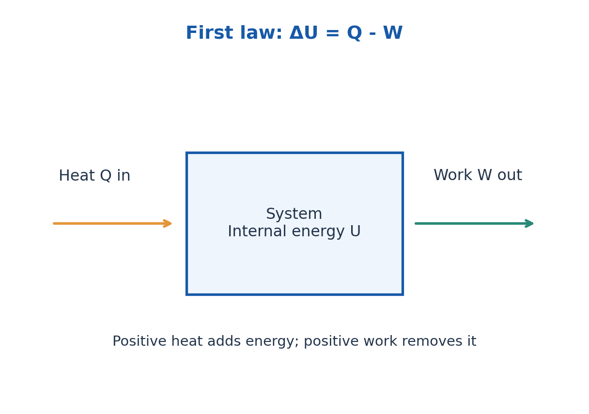
Using work done by the system as positive, the first law is ΔU = Q – W. For a quasistatic expansion W = ∫p dV. Constant-volume heating has no boundary expansion work, whereas an isothermal ideal-gas expansion can absorb heat while maintaining constant internal energy. State the sign convention before calculating.
The second law sets the direction of spontaneous processes and limits heat-engine efficiency. For a reversible transfer dS = δQrev/T; total entropy generation is nonnegative. A heat engine between reservoirs TH and TC cannot exceed Carnot efficiency 1 – TC/TH, with temperatures in kelvin.
The third law concerns the limiting entropy of a perfect crystal as temperature approaches absolute zero. Absolute zero cannot be reached by a finite sequence of ordinary cooling operations. Engineering thermal processes must satisfy energy conservation and the direction imposed by entropy generation.
Worked Problem 3.28: First-Law Sign Convention
Problem: A closed system receives 900 J of heat and does 350 J of work. Find ΔU.
Method: ΔU = Q – W for positive work done by the system.
Calculation: ΔU = 900 – 350.
Answer: ΔU = +550 J.
Check: Work done on the system would enter with the opposite sign in this convention.
23. Conduction, Convection and Radiation – ME and TX
Fourier’s law for one-dimensional conduction is qz = -k dT/dz, where qz is heat flux in W/m² and k is thermal conductivity in W/(m K). Heat flows down the temperature gradient. For a uniform slab at steady state, heat rate is kA(Th – Tc)/L and thermal resistance is L/(kA).
Convection transfers heat between a surface and a moving fluid. Newton’s law is Qdot = hA(Ts – Tfluid). The coefficient h depends on flow and geometry and is not the same as material conductivity k. Wind can increase convective exchange but does not necessarily cool a surface below the air temperature without another energy sink.
Thermal radiation does not require a material medium. For a small grey surface exchanging with large isothermal surroundings, Qdot = εσSB A(Ts^4 – Tsur^4). All temperatures must be absolute. Emissivity is between zero and one under the stated spectral/total convention.
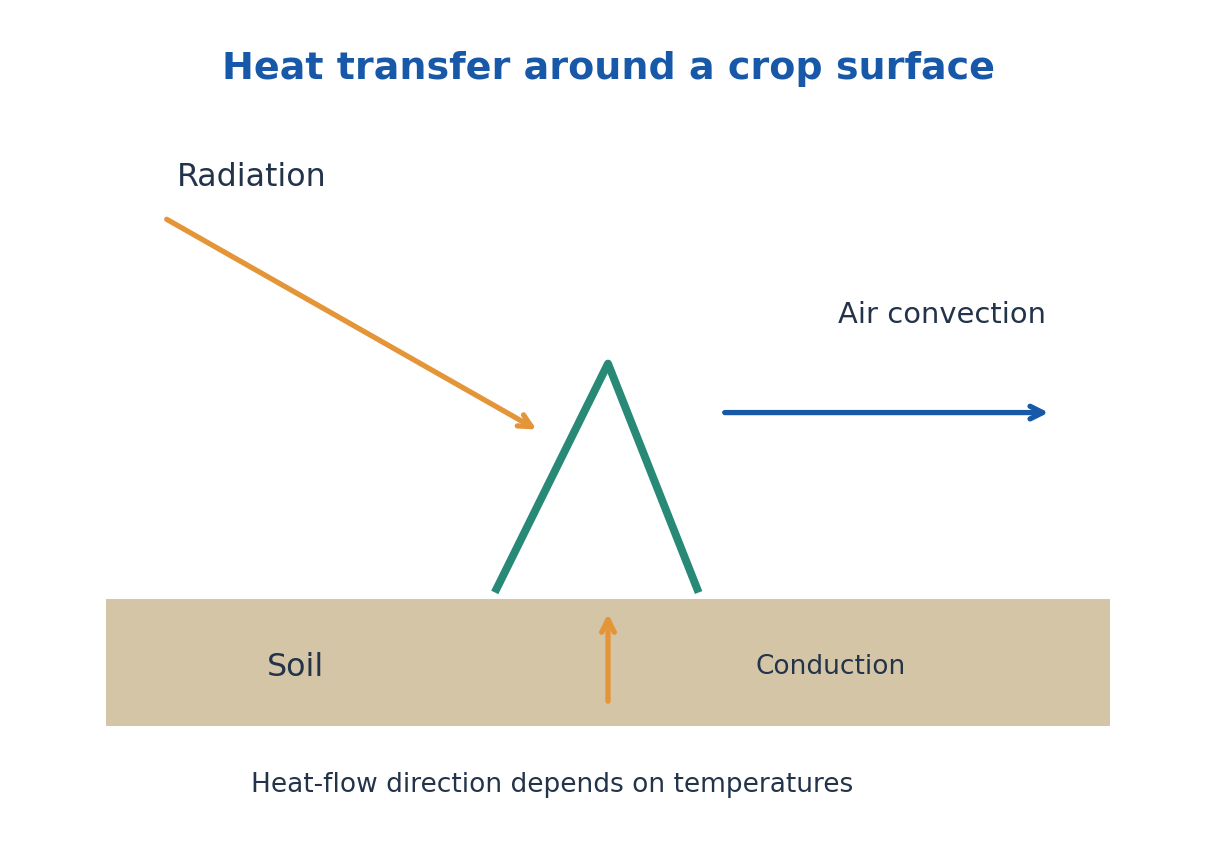
Conduction, convection and radiation usually act together around plants and protected cultivation. Mulch changes radiation absorption, contact resistance and evaporation as well as conduction. A formula for one mechanism is not automatically the complete field energy balance.
Worked Problem 3.29: Two-Layer Steady Conduction
Problem: Two slabs of equal area 1.0 m² have L1 = 0.10 m, k1 = 0.50 W/(m K), L2 = 0.05 m and k2 = 0.25 W/(m K). End temperatures differ by 20 K. Find heat rate.
Method: Series thermal resistances add.
Calculation: R1 = 0.20 K/W, R2 = 0.20 K/W; Qdot = 20/0.40.
Answer: Heat rate = 50.0 W.
Check: The steady heat rate is the same through both series layers, not the sum of two independently imposed rates.
24. Heat Capacity, Conductivity and Thermal Expansion
Heat capacity C = dQ/dT under a specified process has units J/K; specific heat c is per unit mass in J/(kg K). For constant-volume and constant-pressure processes the capacities can differ because work differs. For an ideal gas per mole, CP – CV = R. For a finite temperature range use Q = m∫c(T)dT, or mcΔT when c is approximately constant.
Thermal conductivity k controls heat flow under a temperature gradient; heat capacity controls stored energy for a temperature change. They are not interchangeable. A material can conduct heat rapidly while storing comparatively little energy per volume. Diffusivity αth = k/(ρc) combines these effects for a simple medium.
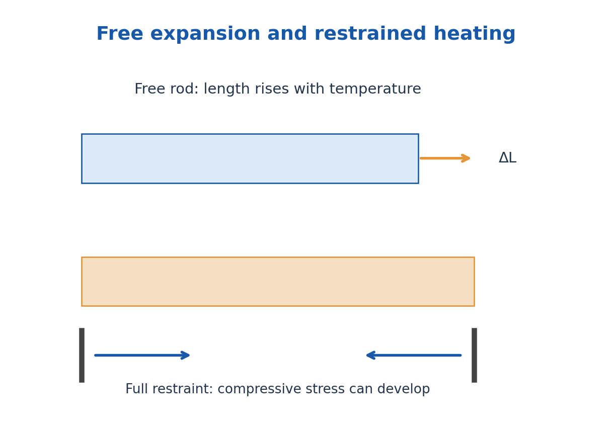
For small temperature changes, linear expansion is ΔL = αL L0ΔT. Isotropic area and volume expansion coefficients are approximately 2αL and 3αL. A hole in a freely expanding plate increases as if the missing material expanded with the plate. Nonuniform temperatures or constraints can produce stress.
ME extension: If a uniform linear elastic rod is completely restrained and would otherwise thermally expand, the axial stress magnitude is approximately YαLΔT, provided yielding, buckling and temperature-dependent changes are negligible. Free expansion produces strain without this constraint stress.
Worked Problem 3.30: Sensible Heat and Capacity
Problem: Heat 2.0 kg of a solid from 20°C to 80°C with constant c = 450 J/(kg K). Find heat and specimen heat capacity.
Method: Q = mcΔT; C = mc.
Calculation: ΔT = 60 K; C = 2 × 450.
Answer: C = 900 J/K; Q = 54000 J = 54.0 kJ.
Check: Specific heat and total specimen heat capacity have different units.
Worked Problem 3.31: Expansion and Restraint
Problem: A 2.0 m steel rod has αL = 12 × 10^-6 K^-1, Y = 200 GPa and temperature rise 50 K. Find free expansion and fully restrained elastic stress magnitude.
Method: ΔL = αL LΔT; |σ| = YαLΔT.
Calculation: Thermal strain = 6.0 × 10^-4; multiply by length or modulus.
Answer: Free expansion = 1.20 mm; fully restrained stress magnitude = 120 MPa, compressive.
Check: The restraint result assumes no buckling, yielding or relaxation; free expansion alone does not create this stress.
25. ME: Phase Change, Enthalpy, Entropy and Equations of State
ME-specific depth. During an ideal phase change at a fixed pressure, a pure substance can absorb or release latent heat without a temperature change. Q = mLf describes fusion and Q = mLv vaporisation under the stated conditions. Heating through a phase boundary usually requires sensible terms before and after the latent term.
Melting absorbs latent energy and solidification releases it. An ideal pure material has a plateau on a suitable temperature-time heating curve at constant pressure. Real alloys can transform over a range. Avoid treating the entire heating input as mcΔT through a phase change.
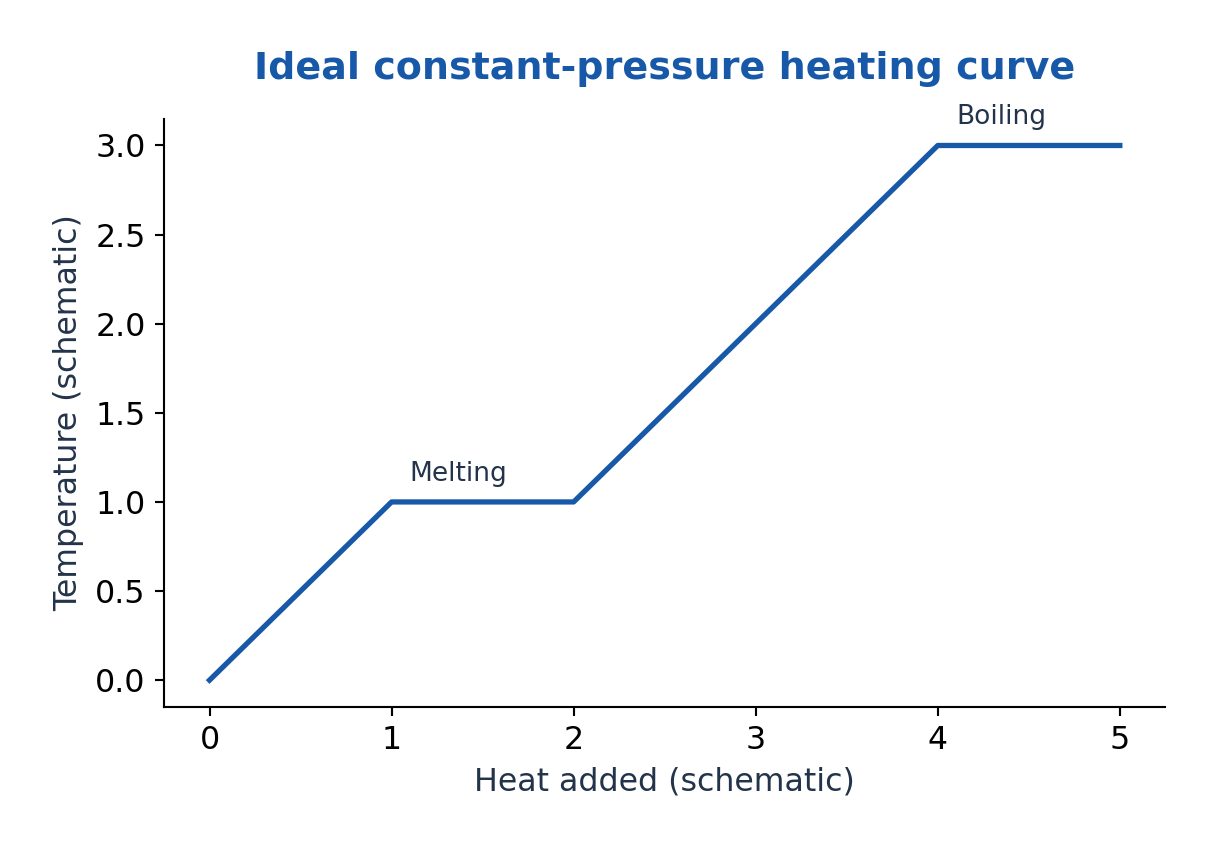
Enthalpy is H = U + pV. At constant pressure with only pressure-volume work, heat transfer equals ΔH. Entropy is a state function with dS = δQrev/T for a reversible path; total entropy generation is nonnegative. For a reversible isothermal phase change, ΔS = mL/T.
An equation of state relates variables such as pressure, volume and temperature. An ideal gas obeys pV = nRT; real gases can deviate at high density or near phase transitions. For one mole, a van der Waals model is (p + a/Vm²)(Vm – b) = RT. The constants correct attractions and finite molecular volume; this is a model, not an exact universal law.
Worked Problem 3.32: Heating and Melting
Problem: Melt 0.50 kg ice initially at -10°C into water at 0°C. Use cice = 2100 J/(kg K) and Lf = 334 kJ/kg. Find heat.
Method: Q = mciceΔT + mLf.
Calculation: Sensible term = 0.50 × 2100 × 10 = 10500 J; latent term = 167000 J.
Answer: Q = 177500 J = 177.5 kJ.
Check: There is no final water-heating term because the specified final temperature is 0°C.
Worked Problem 3.33: Entropy and Equation of State
Problem: For reversible melting of 0.10 kg ice at 273.15 K with Lf = 334 kJ/kg find ΔS. Separately find pressure of 1.0 mol ideal gas at 300 K in 0.0240 m³.
Method: ΔS = mLf/T; p = nRT/V.
Calculation: Use absolute temperatures and R = 8.314462618 J/(mol K).
Answer: ΔS = 122.2771 J/K; gas pressure = 103.9308 kPa.
Check: These are separate examples. Entropy is not heat itself; the gas estimate assumes ideal behaviour.
26. ME: Thermal Resistance and Newton Law of Cooling
In one-dimensional steady conduction through a uniform slab, thermal resistance is Rth = L/(kA) and heat rate is ΔT/Rth. Resistances in series add. A convective film has resistance 1/(hA). Contact resistance or radiation can add other paths; the correct network follows the actual physical boundaries.
Newton’s cooling law in lumped form gives mc dT/dt = -hA(T – T∞) when h, area, heat capacity and surroundings are constant and internal temperature gradients are negligible. The solution is T – T∞ = (T0 – T∞)exp(-t/τth), with τth = mc/(hA).
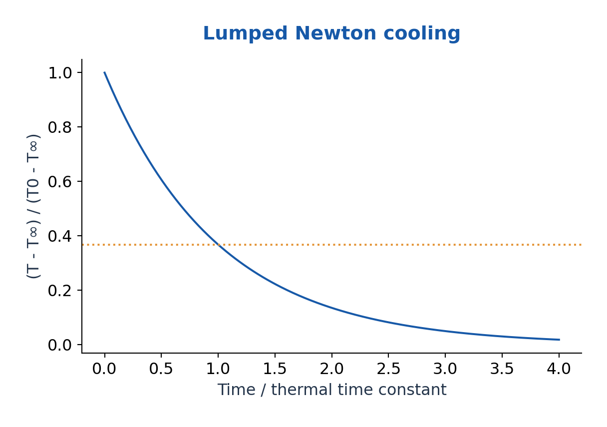
The lumped approximation is commonly checked by Bi = hLc/k much less than one, often using Bi < 0.1 as a practical criterion with characteristic length Lc = V/A. This concerns internal uniformity; it is not a statement that cooling is always slow.
For radiative cooling over a large temperature range, heat rate is not simply proportional to Celsius temperature difference; use the fourth-power law or a justified local linearisation.
A measured cooling curve can estimate a model parameter, but heat leaks, evaporation and changing airflow may invalidate a single exponential fit.
Worked Problem 3.34: Newton Cooling Time
Problem: An ideal lumped body has τth = 600 s. It cools from 80°C toward surroundings at 20°C. Find time to reach 40°C.
Method: (T – T∞)/(T0 – T∞) = exp(-t/τth).
Calculation: Final difference ratio = 20/60 = 1/3; t = 600 ln3.
Answer: t = 659.1674 s = 10.9861 min.
Check: The ratio uses temperature differences; the exponential model requires constant surroundings and approximately uniform body temperature.
27. F. Newton Laws and Equilibrium – CE
Newton’s first law defines inertial motion when net external force is zero. The second law is net force equal to rate of momentum change; for constant mass, ΣF = ma. The third law pairs equal and opposite interaction forces on different bodies, so the pair does not cancel on one body’s free-body diagram.
Static equilibrium requires zero net external force and zero net torque about a convenient point. Dynamic equilibrium can describe constant-velocity motion with zero acceleration; in engineering force-balance treatments an inertia term -ma may be introduced using d’Alembert’s principle. State which meaning and reference frame you use.
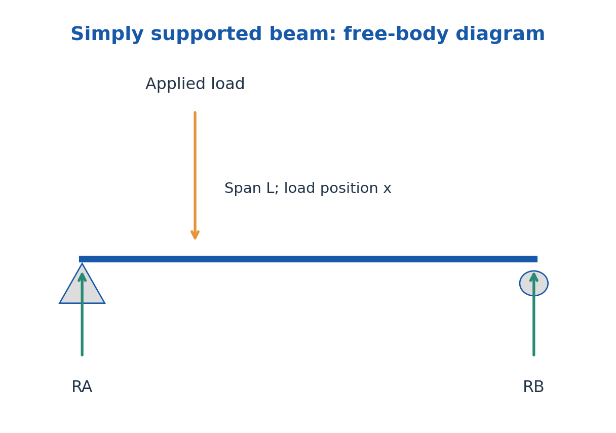
A free-body diagram isolates one selected body and shows its external loads, weight, support reactions and applied couples. Choose axes, resolve forces, then write force and moment equations. Internal forces between parts of a combined system do not appear as external loads on that entire system.
A body can have zero resultant force but a nonzero torque and therefore rotate. Conversely, choosing a moment centre at a support can eliminate unknown reaction moments from that equation without eliminating the forces from the full problem. Check both translation and rotation.
Worked Problem 3.35: Beam Reactions
Problem: A massless simply supported beam spans 4.0 m. A 600 N downward point load acts 1.0 m from the left support. Find vertical reactions.
Method: ΣFy = 0 and moment balance about the left support.
Calculation: RB × 4 = 600 × 1, so RB = 150 N; RA = 600 – 150.
Answer: RA = 450 N upward; RB = 150 N upward.
Check: Reactions sum to the load and their moments balance. Beam self-weight is excluded by the given model.
28. Stress, Strain and Hooke Law – CE
Engineering normal stress is force divided by original cross-sectional area: σ = F/A0. Tensile stress stretches a specimen; compressive stress shortens it under the chosen sign convention. Stress has units N/m² = Pa. One MPa equals one N/mm².
Engineering longitudinal strain is ε = ΔL/L0. It is dimensionless and may be expressed as a fraction, percent or microstrain. A value 0.001 is 0.1%, not 1%. Keep original and deformed dimensions distinct when a problem asks for engineering rather than true measures.
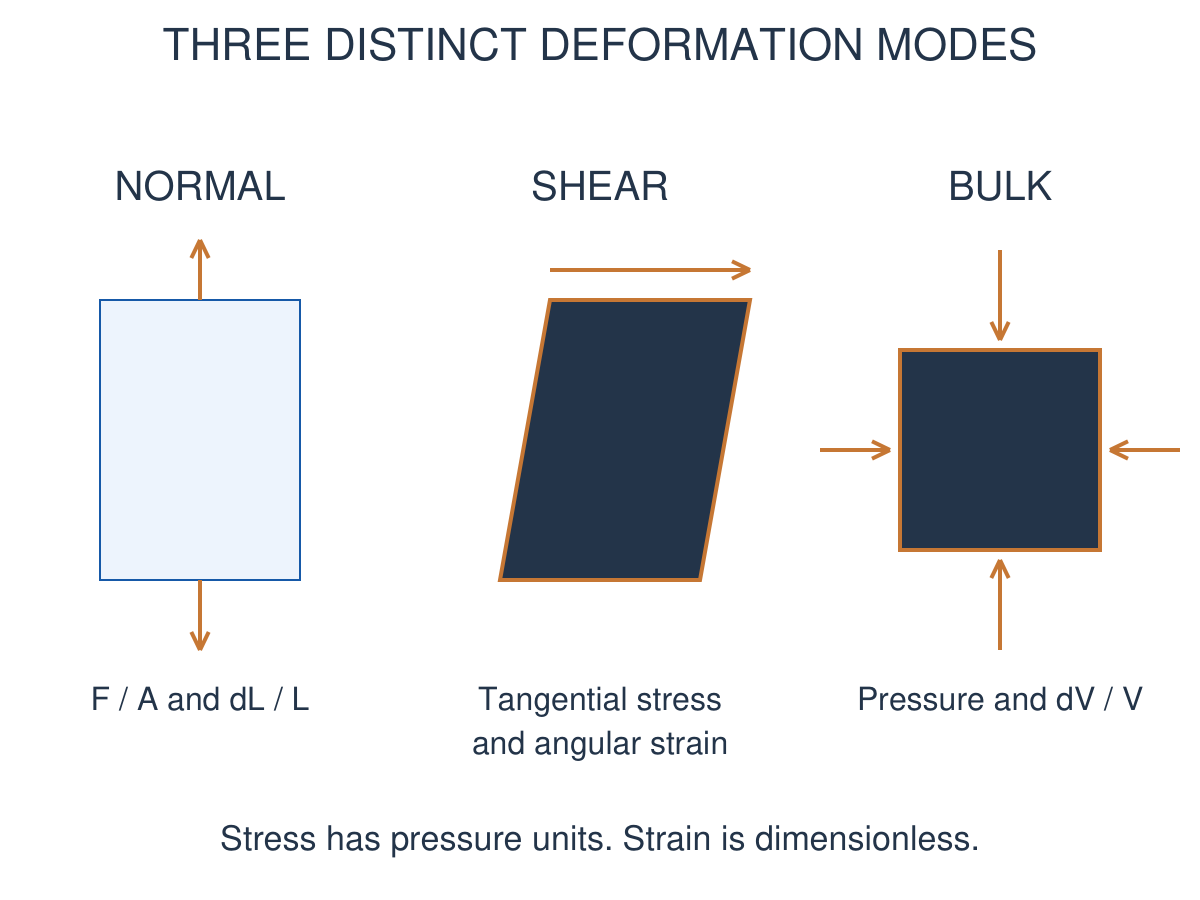
Shear stress is tangential force divided by the relevant area. For a small simple shear, strain γ ≈ lateral displacement/height ≈ shear angle in radians. Volumetric strain is ΔV/V; its sign depends on whether compression is represented as negative or by a positive magnitude.
Elastic deformation is recovered on unloading within the relevant regime. Linear elasticity is the more restrictive region where stress is proportional to strain. Elastic does not automatically mean exactly linear up to every load.
Worked Problem 3.36: Uniaxial Elastic Extension
Problem: A rod of length 1.0 m and area 20 mm² carries tensile force 2000 N. Y = 200 GPa. Find stress, strain and extension.
Method: σ = F/A; ε = σ/Y; ΔL = εL.
Calculation: Area = 20 × 10^-6 m²; σ = 10^8 Pa.
Answer: Stress = 100 MPa; strain = 5.00 × 10^-4; extension = 0.500 mm.
Check: The Young-modulus relation assumes the stated linear elastic regime.
29. Young, Bulk and Shear Moduli – CE
Young modulus Y is normal stress divided by longitudinal strain in a uniaxial linear elastic test: Y = σ/ε = FL0/(A0ΔL). It measures stiffness of the material, while a component’s extension also depends on its dimensions.
Bulk modulus K measures resistance to volume change under hydrostatic pressure: K = -Δp/(ΔV/V) for a sufficiently small change. With compression magnitudes, K = Δp/|ΔV/V|. The minus sign makes K positive for ordinary stable materials.
Shear modulus G is shear stress divided by shear strain in the linear regime: G = τ/γ. It measures resistance to shape change rather than direct hydrostatic volume compression. All three moduli have pressure units.
Poisson ratio νP is minus transverse strain divided by axial strain in a uniaxial test. For a homogeneous isotropic linear elastic material, Y = 2G(1 + νP) = 3K(1 – 2νP) and Y = 9KG/(3K + G). Do not impose these isotropic formulas blindly on direction-dependent single-crystal properties.
Worked Problem 3.37: Hydrostatic Compression Modulus
Problem: A pressure rise 20 MPa produces volume strain -2.0 × 10^-4. Find K.
Method: K = -Δp/(ΔV/V).
Calculation: Divide positive pressure rise by the magnitude of volume contraction.
Answer: K = 100 GPa.
Check: The minus sign ensures positive bulk modulus for an ordinary stable compressive response.
30. Fluid Properties, Hydrostatics and Archimedes Principle – CE
A fluid cannot sustain a static shear stress without continuing deformation. Density is ρ = m/V, specific volume is 1/ρ and specific gravity is a density ratio. Compressibility measures volume response to pressure. Liquids are often approximately incompressible over modest pressure ranges; gases generally need an equation of state.
Pressure is normal compressive force per area. In a static liquid, dp/dz = -ρg when z increases upward. For constant density, pressure rises by ρgh at depth h. Absolute pressure equals gauge pressure plus atmospheric pressure. A negative gauge pressure does not automatically imply a negative absolute pressure.
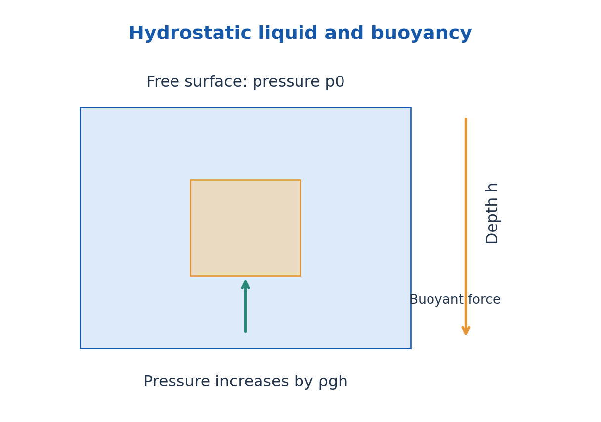
Pascal’s principle describes the transmission of an applied pressure increment through a confined static fluid. In a hydraulic press, F1/A1 = F2/A2 for equal elevations and negligible losses. Force amplification comes with a corresponding displacement change; it does not create energy.
Archimedes’ principle gives upward buoyancy equal to the weight of displaced fluid, FB = ρfluid g Vdisplaced. A floating object displaces its own weight. For a uniform object floating in one liquid, the submerged fraction is ρobject/ρfluid. Use displaced volume, which need not be the entire object volume.
Worked Problem 3.38: Buoyancy and Submerged Fraction
Problem: A uniform 720 kg/m³ block floats in water of density 1000 kg/m³. Find submerged fraction and buoyancy for total volume 0.0100 m³.
Method: Floating buoyancy equals weight; Vsub/V = ρblock/ρwater.
Calculation: Mass = 720 × 0.0100 = 7.20 kg; use g = 9.81 m/s².
Answer: Submerged fraction = 0.720; buoyancy = 70.632 N.
Check: Only 0.00720 m³ of water is displaced, not the entire object volume.
31. Viscosity, Surface Tension and Capillarity – CE
Dynamic viscosity μ relates Newtonian simple-shear stress to velocity gradient: τs = μ du/dy. Kinematic viscosity is ν = μ/ρ. A fluid may be approximately incompressible without having zero viscosity; inviscid and incompressible are separate assumptions.
Surface tension γ acts tangentially along an interface. Its dimensions N/m equal J/m². A spherical liquid drop has one curved interface and excess pressure 2γ/r. A thin soap bubble has two interfaces and excess pressure approximately 4γ/r.
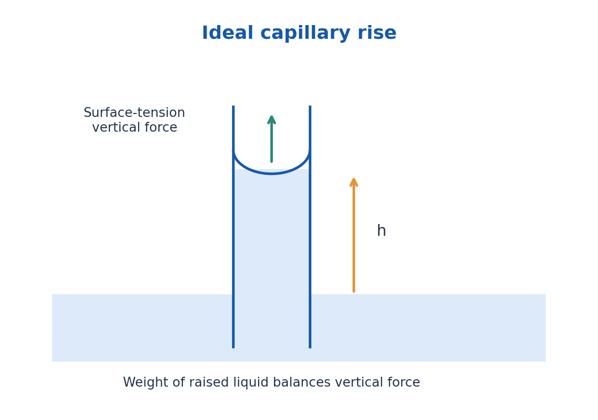
In an ideal circular capillary, vertical interfacial force 2πrγ cosθ balances raised-liquid weight ρgπr²h, yielding h = 2γ cosθ/(ρgr). The angle is measured through the liquid. Wetting can cause rise and non-wetting can cause depression. A smaller radius gives a greater ideal equilibrium height.
Civil applications include capillary moisture movement, coatings, drainage and fluid transport. Real pore networks add tortuosity, contact-angle variation and nonuniform sizes. The equilibrium capillary formula does not determine all time-dependent moisture migration in a wall or soil.
Worked Problem 3.39: Capillary Radius and Rise
Problem: A fully wetting liquid has γ = 0.072 N/m and ρ = 1000 kg/m³. Find rise in a tube of diameter 1.0 mm.
Method: h = 4γ/(ρgd) for θ = 0.
Calculation: Use d = 0.0010 m and g = 9.81 m/s².
Answer: h = 29.3578 mm.
Check: Diameter in this expression replaces twice the radius; using it directly in the radius form halves the answer.
32. Bernoulli Equation and Continuity – CE
Steady mass conservation gives ρ1A1v1 = ρ2A2v2 for one inlet and one outlet without leakage or accumulation. For an incompressible fluid, Q = Av is constant, so narrowing the area increases mean speed. A velocity field can vary even when the material density is constant.
For steady, incompressible, inviscid flow along a streamline, Bernoulli’s equation is p + ρv²/2 + ρgz = constant. It expresses mechanical energy per volume; dividing by ρg gives pressure, velocity and elevation heads. For rotational flow the constant can differ between streamlines.
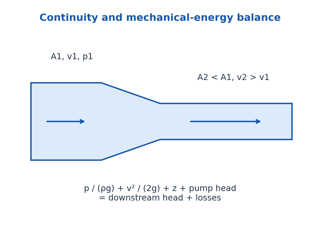
For engineering pipe systems include pumps, turbines and head loss: p1/(ρg) + v1²/(2g) + z1 + hp = p2/(ρg) + v2²/(2g) + z2 + ht + hL. Irreversible loss is nonnegative along the flow. Real viscous pipes do not obey loss-free Bernoulli over an arbitrary length.
A Venturi uses continuity and a pressure difference to infer flow under a specified discharge coefficient. A Pitot tube relates stagnation and static pressure to local speed when the assumptions apply. Check elevations and whether the question asks static pressure, stagnation pressure or head.
33. CE: Flow Through Pipes and Regime Checks
Steady incompressible flow has Q = Av. In a circular pipe, Reynolds number Re = ρvD/μ uses mean speed and internal diameter. A common laminar criterion is Re below about 2300 for a conventional circular pipe, with a disturbance-dependent transition region.
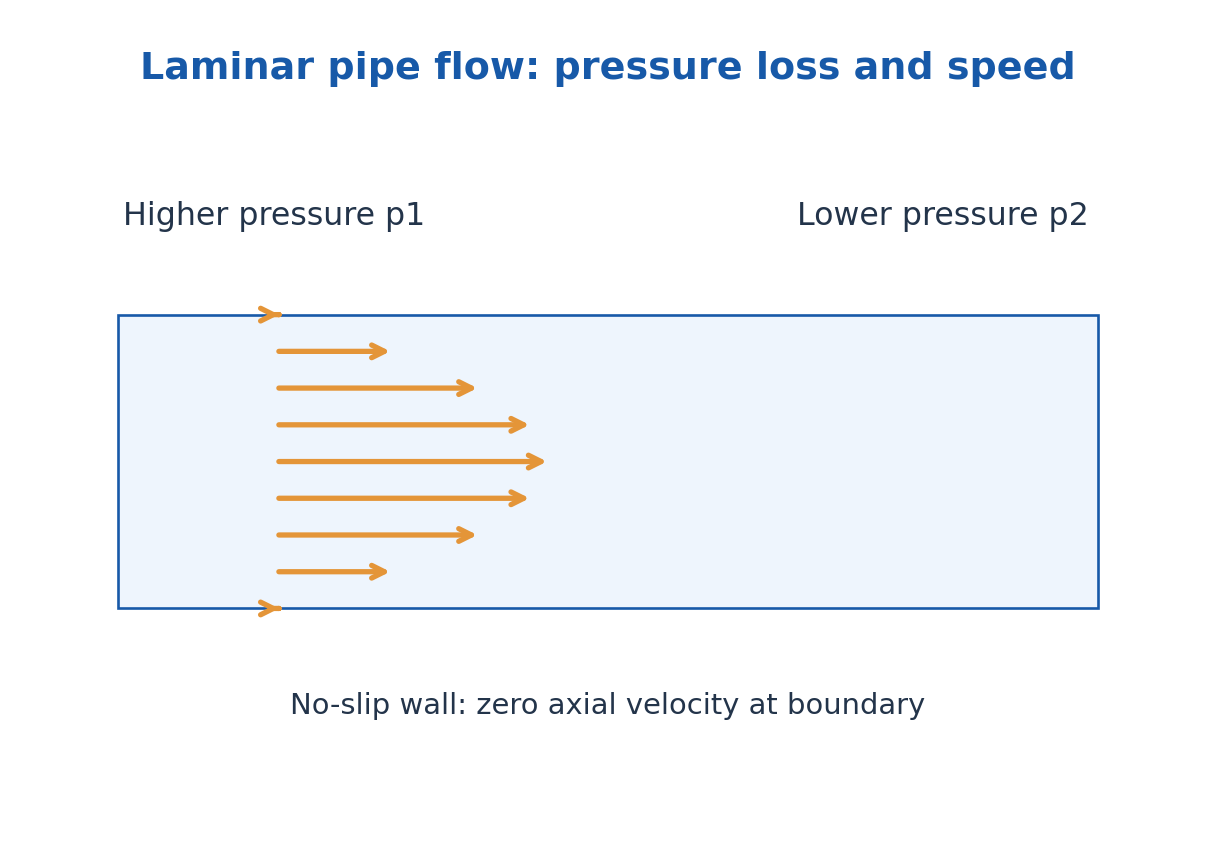
For fully developed laminar flow of a Newtonian liquid with no slip, the axial velocity profile is parabolic and vmax = 2vmean. Volume flow is Q = πR^4 Δp/(8μL), or pressure drop Δp = 32μLvmean/D². Use the tube radius in the fourth-power formula and diameter in the latter form.
Darcy-Weisbach gives head loss hL = fD(L/D)v²/(2g); laminar circular flow has Darcy factor fD = 64/Re. Turbulent flow requires a suitable friction relation and roughness. Fanning and Darcy friction factors differ by a factor four, so the convention must be declared.
Include pump head, elevation, kinetic-head changes and losses in a complete pipe energy balance. Minor-loss coefficients describe bends and fittings in the selected convention. If a calculated flow violates the assumed laminar regime, the first solution is not self-consistent.
Worked Problem 3.40: Laminar Pipe Flow
Problem: Water with μ = 0.001 Pa s and ρ = 1000 kg/m³ flows at mean 0.10 m/s in a 10 mm diameter, 5.0 m long pipe. Find Re and pressure loss.
Method: Re = ρvD/μ; Δp = 32μLv/D².
Calculation: Re = 1000, consistent with the laminar model; substitute the SI diameter 0.010 m.
Answer: Re = 1000; pressure loss = 160 Pa.
Check: A loss-free Bernoulli calculation along this constant-diameter horizontal pipe would miss the viscous pressure drop.
34. G. Superconductivity: Transition and Critical Field – AG
A superconductor has zero DC resistivity in its superconducting regime and exhibits the Meissner effect. Superconductivity is a thermodynamic phase with limits in temperature, magnetic field and current density; lowering the temperature below Tc alone does not ensure every operating condition is permissible.
Resistivity changes from the finite normal-state value to zero at the transition in an ideal measurement. Real transitions can have width from material or measurement conditions. A persistent current can circulate without ordinary resistive decay in a suitable superconducting closed loop, although external disturbances and flux motion can still matter.
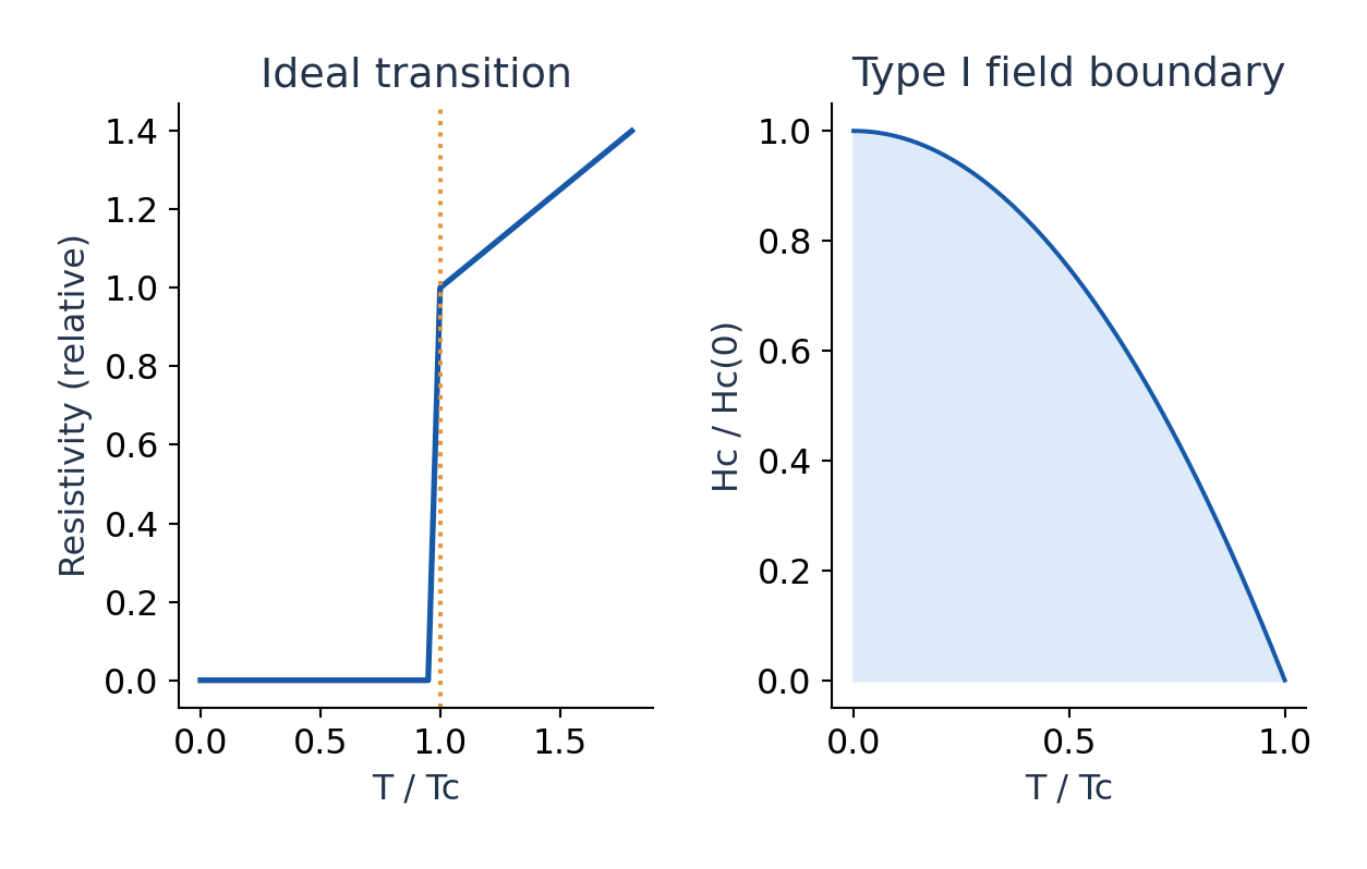
For an introductory Type I model the thermodynamic critical field follows Hc(T) ≈ Hc(0)[1 – (T/Tc)²]. The field tends to zero near Tc and increases on cooling. If the given critical quantity is Bc in tesla instead, apply the same supplied temperature law consistently rather than mixing B and H units.
The Meissner effect expels magnetic flux from the bulk of a suitable specimen in the superconducting phase, apart from a finite penetration layer and geometry effects. A perfect conductor would preserve its initial flux under ideal assumptions, so zero resistance alone does not establish the Meissner property.
Worked Problem 3.41: Critical Field at Temperature
Problem: A Type I model has Tc = 10.0 K and Bc(0) = 0.080 T. Find Bc at 6.0 K under Bc(T) = Bc(0)[1 – (T/Tc)²].
Method: Apply the explicitly supplied Bc temperature law.
Calculation: T/Tc = 0.6; factor = 1 – 0.36 = 0.64.
Answer: Bc(6 K) = 0.0512 T.
Check: A field above this model boundary would not lie in its superconducting region; no B-to-H unit substitution is needed here.
Worked Problem 3.42: Temperature for a Specified Critical Field
Problem: Using the same model, find T where Bc is half of Bc(0).
Method: 1 – (T/Tc)² = 1/2.
Calculation: T = Tc/√2.
Answer: T = 7.07107 K.
Check: The positive root is used and lies below Tc.
35. Type I, Type II, High-Temperature Materials and Applications
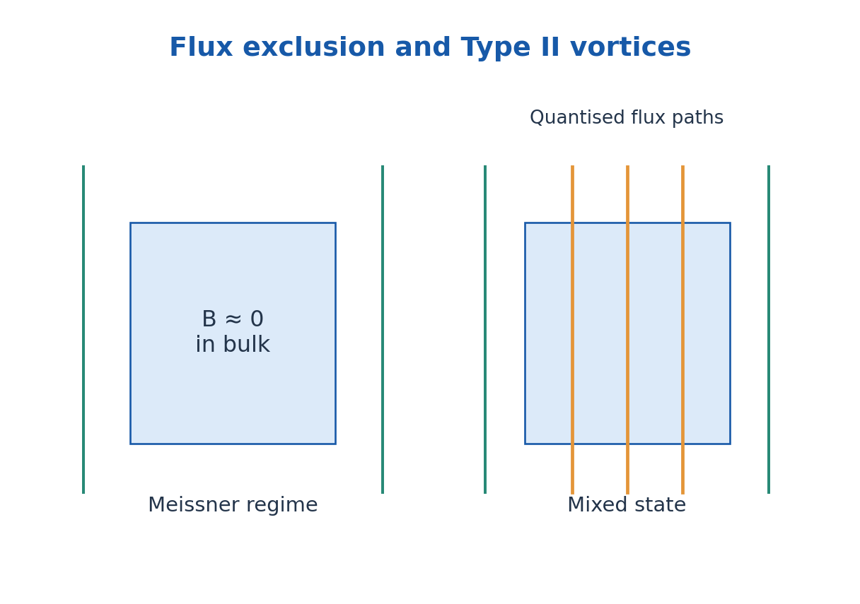
Type I superconductors have one thermodynamic critical field separating the ideal Meissner and normal regimes, with demagnetisation-dependent intermediate states possible. Type II superconductors have lower and upper critical fields Hc1 and Hc2. Between them, a mixed state admits quantised vortices while superconductivity persists in other regions.
Below Hc1 the ideal bulk is in a Meissner regime. Above Hc2 superconductivity is lost. Pinning can restrain vortex motion and support useful current with low dissipation; unrestrained vortex movement can produce loss. Type II does not mean the material never expels flux.
High-temperature superconductors have transition temperatures high relative to conventional low-temperature systems; many are ceramic compounds and some operate above liquid-nitrogen temperature. The label does not imply room-temperature operation, ordinary wiring convenience or absence of cooling and mechanical constraints.
Applications include high-field magnets, sensitive magnetic measurements, low-loss electrical components and specialised sensors. Agricultural connections can include advanced analytical instruments, but one should not claim an ordinary farm motor or soil probe is superconducting. Practical selection includes cooling, critical current, magnetic field, cost and material durability.
Worked Problem 3.43: Type II Regime Identification
Problem: At a stated temperature a Type II specimen has μ0Hc1 = 0.030 T and μ0Hc2 = 5.0 T. Identify the ideal bulk regimes at applied μ0H = 0.010, 0.50 and 6.0 T, neglecting geometry effects.
Method: Compare with both critical bounds.
Calculation: 0.010 < 0.030; 0.030 < 0.50 < 5.0; 6.0 > 5.0.
Answer: Meissner, mixed/vortex and normal regimes respectively.
Check: The middle field does not mean superconductivity has vanished; current and pinning limits also matter in practice.
36. Nanomaterials: Size, Surfaces and Material Properties
Nanomaterials have at least one relevant dimension in the nanoscale range, often roughly 1–100 nm in an introductory definition. Behaviour can change because surface-to-volume ratio rises and because electron, phonon or other characteristic lengths become comparable to dimensions. Not every property changes in the same way for every material.
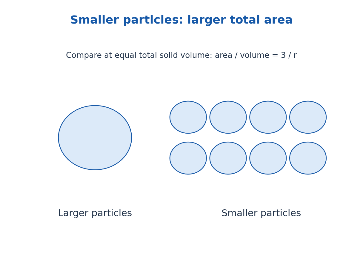
For a sphere, surface-to-volume ratio is 3/r. Halving radius doubles that ratio for the same ideal geometry. A larger fraction of atoms near surfaces can change chemical activity, melting behaviour, adsorption and mechanical response. Surface chemistry and agglomeration matter as much as nominal particle diameter in many applications.
Quantum confinement can make energy levels depend on size and dimensionality. Optical absorption and emission may shift when a semiconductor particle becomes sufficiently small relative to its relevant quantum length. A classical metal nanoparticle can also show collective-electron optical response; these are different mechanisms.
Useful properties include tunable optical response, large interface area and modified transport or mechanical behaviour. Applications include sensing, coatings, catalysts and controlled-delivery research. Performance must be evaluated for a stated material and environment; nanoscale size alone does not prove safety, selectivity or environmental benefit.
Worked Problem 3.44: Nanoparticle Surface Area
Problem: Compare ideal separated spheres of radii 50 nm and 10 nm with the same total solid volume. Find the total surface-area ratio.
Method: For fixed total volume, total area/volume = 3/r.
Calculation: Area ratio Asmall/Alarge = 50/10.
Answer: Smaller spheres provide five times the total external area.
Check: This comparison holds total volume, not particle number, fixed and neglects agglomeration.
37. Quantum Wells, Wires, Dots and Nanofabrication – AG
A quantum well confines carrier motion strongly in one direction while allowing approximate motion in two; a quantum wire confines two directions and leaves one extended; a quantum dot confines all three. These names count confined directions, not the visible shape of a macroscopic device. The remaining extended dimensions influence the density of states.
An ideal infinite well gives a confinement-energy scale proportional to 1/L². Real nanostructures have finite barriers, effective masses, interactions and interface imperfections, so the elementary model supplies trends rather than a universal numerical spectrum. Size distribution can broaden an ensemble’s optical response.
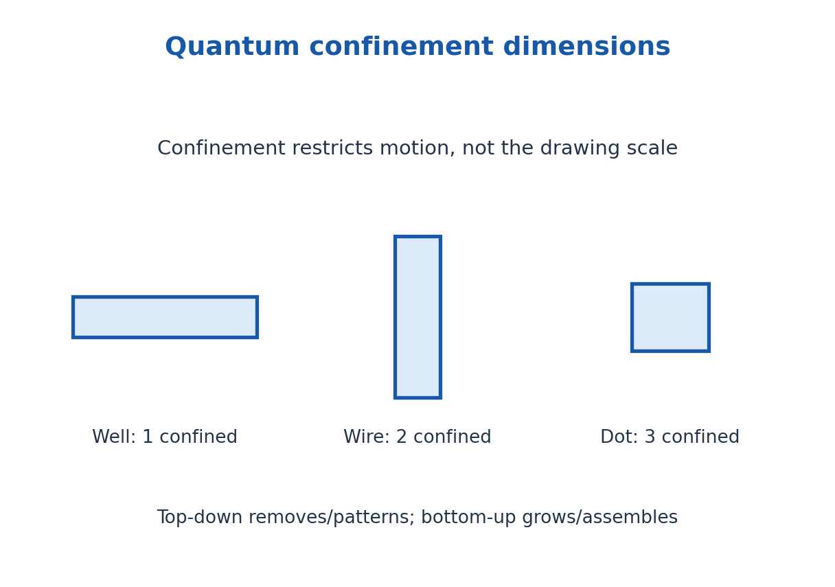
Top-down fabrication begins with larger material and patterns or removes portions by methods such as lithography, etching or milling. Bottom-up approaches assemble structures from atoms, molecules or precursors by growth, deposition or self-assembly. A practical device can use both approaches.
In agriculture, investigated nanomaterial applications include sensing, water-treatment media, protective coatings and nutrient or pesticide carriers. Evaluate release rate, exposure, persistence and field performance rather than assuming that laboratory performance guarantees a beneficial field outcome. This route includes nanofabrication because AG lists it explicitly.
Worked Problem 3.45: Confinement and Fabrication Classification
Problem: An ideal confined dimension decreases from 8 nm to 4 nm. Find the confinement-energy factor. Classify etching a patterned bulk wafer and growing dots from precursors.
Method: Confinement scale ∝ 1/L².
Calculation: Enew/Eold = (8/4)².
Answer: Energy scale rises by factor four; patterned etching is top-down and precursor growth is bottom-up.
Check: Real barriers, effective masses and interactions can change absolute energies; the answer states an ideal scaling model.
38. H. Classical Limitations, Matter Waves and Diffraction – CH
Classical physics remains effective for many macroscopic motions, but cannot fully explain measured thermal radiation, threshold photoelectric emission, stable atomic spectra and electron diffraction. Quantum theory introduces states, probabilities and quantised exchanges where these observations require them. A correct answer connects each failed classical prediction with the relevant experiment.
De Broglie wavelength is λ = h/p. For a non-relativistic particle, λ = h/√(2mK); an electron accelerated from rest through voltage magnitude V has K = eV and λ ≈ 1.2264/√V nm. Matter waves describe quantum amplitudes and can propagate in vacuum; they are not mechanical disturbances requiring a material medium.
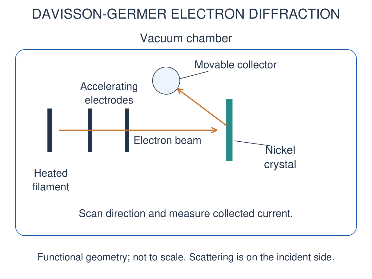
Davisson and Germer directed accelerated electrons at a nickel crystal in vacuum and measured scattered intensity with a movable collector. Diffraction maxima gave a wavelength consistent with the momentum prediction. The crystal provides ordered scattering sites, not a visible set of macroscopic slits.
Bragg constructive interference is nλ = 2d sinθ with θ measured from the lattice plane. For the familiar 54 V illustration, a convention with a 50° collector angle gives a 65° Bragg glancing angle. Using d = 0.091 nm gives about 0.165 nm, close to the de Broglie value about 0.167 nm. Do not substitute the collector angle directly without checking geometry.
Worked Problem 3.46: Electron Wavelength After Acceleration
Problem: An electron starts nearly at rest and gains 100 eV. Find its non-relativistic wavelength.
Method: λ = h/√(2mK); K = 100e joules.
Calculation: Use electron mass and convert eV to joules before substitution.
Answer: λ = 0.12264 nm.
Check: 100 eV is small relative to the electron rest energy, supporting the non-relativistic estimate.
39. Wave Packets, Phase Velocity and Group Velocity – CH
A single sinusoid extends through space. A localised packet superposes a range of wave numbers. Write each component as exp[i(kx – ωt)], with p = ħk and E = ħω in the stated energy convention. Superpose amplitudes first and then take a squared magnitude to obtain interference probabilities.
For two nearby components, the carrier phase travels at vp = ω/k and the envelope at Δω/Δk, approaching vg = dω/dk. Since ω = kvp, vg = vp + k dvp/dk = vp – λ dvp/dλ. A dispersive medium or particle relation can also cause packet spreading.
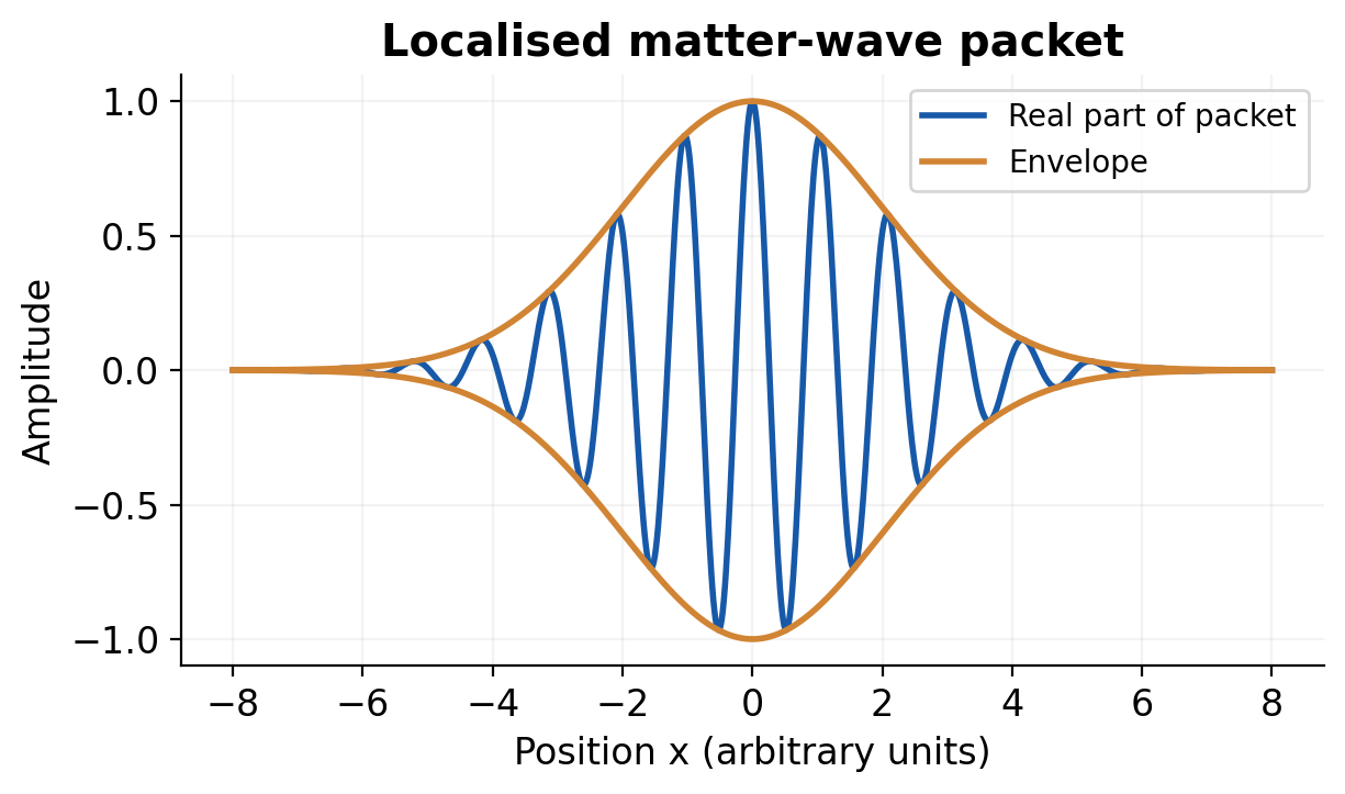
With non-relativistic free-particle kinetic energy E = p²/(2m), ω = ħk²/(2m); thus vp = v/2 and vg = v. With total relativistic energy, vp = c²/v while vg = v. These phase-speed expressions use different energy conventions; a phase speed greater than c does not by itself transmit a chosen signal faster than c.
Increasing spatial localisation generally requires a broader wave-number spread. A packet is not a rigid envelope in every medium or for every time. Distinguish carrier crests, envelope motion and changes in envelope width when describing a labelled plot.
Worked Problem 3.47: Free-Particle Packet Speeds
Problem: A non-relativistic electron has group speed 2.0 × 10^6 m/s. Under a kinetic-energy-only dispersion find phase speed and k.
Method: vg = v; vp = v/2; k = mv/ħ.
Calculation: Use the stated non-relativistic dispersion, not total relativistic phase energy.
Answer: vp = 1.0 × 10^6 m/s; k = 1.7276 × 10^10 m^-1.
Check: Changing the energy-zero convention can change phase evolution but does not change this free-particle group speed.
40. Heisenberg Uncertainty and Applications – CH
The same-direction standard deviations satisfy σxσp ≥ ħ/2. This is a property of quantum state distributions, not merely poor instruments disturbing a pre-existing precise trajectory. A percentage uncertainty must first be translated into an absolute momentum spread if it is to represent σp.
A proof uses Cauchy-Schwarz on (x – ⟨x⟩)ψ and (p – ⟨p⟩)ψ, with the commutator [x,p] = iħ and suitable boundary behaviour. Their squared norms are σx² and σp²; the imaginary part of the inner product supplies ħ/2, yielding the bound. A suitable Gaussian can attain equality, while a generic state need not.
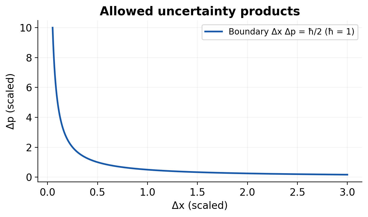
Localising a particle strongly increases its required momentum scale and hence its kinetic-energy scale. This motivates finite atomic dimensions and nonzero confinement energy. For nuclear-length electron localisation, the inferred momentum can require relativistic energy rather than p²/(2m). Zero mean momentum does not mean zero momentum spread.
Energy-time relations need an explicitly stated time and width convention. In an exercise supplying ΔE Δt ≥ ħ/2, use that convention; do not label the result a spectral full width without justification. Such relations do not permit arbitrary violation of energy conservation.
Worked Problem 3.48: Minimum Momentum Spread
Problem: A state has σx = 0.100 nm. Find the lower bound on σp and the corresponding non-relativistic electron σv.
Method: σp ≥ ħ/(2σx); σv = σp/m.
Calculation: Convert width to 1.00 × 10^-10 m.
Answer: σp ≥ 5.2729 × 10^-25 kg m/s; σv ≥ 5.7884 × 10^5 m/s.
Check: Equality is not guaranteed for an arbitrary state; these are spreads rather than definite trajectory values.
41. Wavefunction Interpretation and Schrodinger Equations – CH
The wavefunction is a generally complex amplitude. Born interpretation assigns density |ψ|² and probability P(a,b) = ∫a to b |ψ|² dx. Normalisation requires total probability one over the declared support. Density has inverse-length units in one dimension; it is not itself a dimensionless interval probability.
A physical state must be normalisable where a bound-state interpretation is intended and obey the Hamiltonian’s boundary conditions. For finite nonsingular potentials, the ordinary wavefunction is continuous with the appropriate derivative matching. An ideal infinite wall is a separate limiting boundary condition, not a generic finite-potential interface.
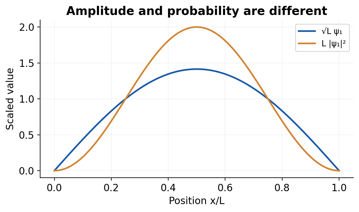
The time-dependent equation is iħ ∂Ψ/∂t = [-ħ²∇²/(2m) + V]Ψ for a non-relativistic particle in the stated potential model. With time-independent V, a stationary state separates as Ψ = ψ exp(-iEt/ħ), giving the time-independent equation -ħ²∇²ψ/(2m) + Vψ = Eψ.
Operators connect states with observables: x acts by multiplication and px = -iħ∂/∂x. An expectation value is a probability-weighted average, such as ⟨x⟩ = ∫ψ*xψ dx. A stationary state’s probability density is time independent even though its global phase evolves. A superposition of different energies can have a changing density.
Worked Problem 3.49: Normalisation and Interval Probability
Problem: A one-dimensional state is ψ = Ax on 0 < x < L and zero elsewhere. Find positive A and the probability in L/2 < x < L.
Method: Integrate |ψ|² = A²x² over the support.
Calculation: 1 = A²L³/3; P(right half) = A²[L³ – (L/2)³]/3.
Answer: A = √(3/L³); right-half probability = 7/8 = 0.875.
Check: Normalise over the full support before evaluating the requested subinterval; A has units length^(-3/2).
42. Particle in a One-Dimensional Box – CH
For an infinite well 0 < x < L, V = 0 inside and infinite outside. The state vanishes at both walls and outside. Inside, the time-independent equation gives sinusoidal solutions; imposing both walls requires kL = nπ with n = 1, 2, 3 and so on. n = 0 gives only the zero function and cannot be normalised.
The normalised spatial eigenstates are ψn = √(2/L)sin(nπx/L), and En = n²h²/(8mL²). Ground energy is nonzero. Increasing width lowers the energy as 1/L²; increasing mass lowers it as 1/m. Adjacent levels are not equally spaced because En scales as n².
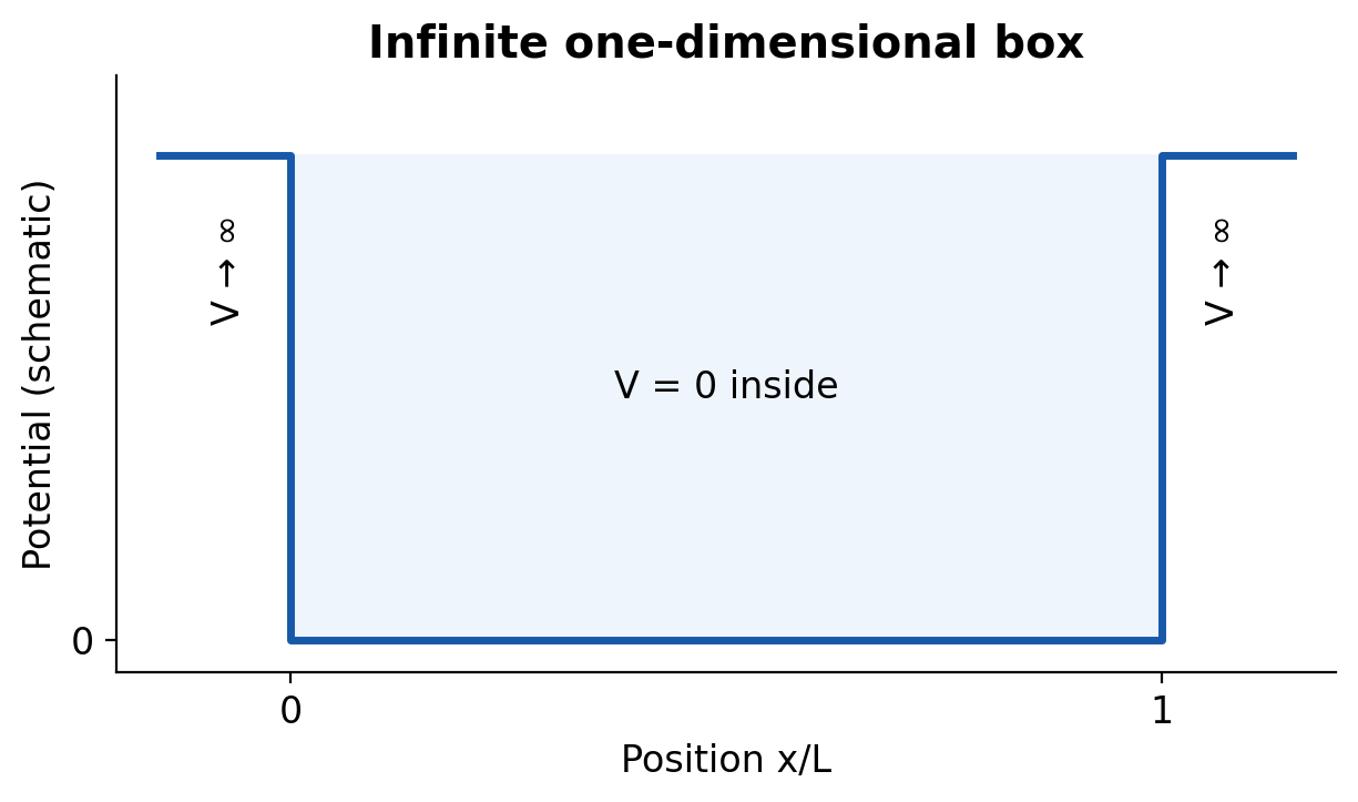
The density has n lobes and n – 1 internal nodes. Each normalised eigenstate has ⟨x⟩ = L/2, but interval probabilities differ with n. The probability of exactly one mathematical point is zero for a continuous density; the density at the centre can nonetheless vanish or be maximal.
For the ideal stationary well, ⟨p⟩ = 0 but ⟨p²⟩ = (nπħ/L)² and kinetic energy is nonzero. A photon emitted in an allowed downward transition has energy equal to the level difference. The ideal well supplies a confinement model; real finite barriers permit penetration and modified levels.
Worked Problem 3.50: Box Energies and a Transition
Problem: An electron occupies a 1.00 nm infinite well. Find E1, E2 and the wavelength for the energy difference E2 – E1 if an allowed radiative transition occurs.
Method: En = n²h²/(8mL²); Eph = 3E1; λph = hc/Eph.
Calculation: Use L = 10^-9 m; E2 = 4E1.
Answer: E1 = 0.37603 eV; E2 = 1.50412 eV; photon wavelength = 1099.0625 nm.
Check: The photon wavelength is not the electron standing-wave wavelength inside the box.
Complete Derivations and Exam Explanations
1. CSE: Prove Bell-State Entanglement and Explain Its Measurement
Begin with a product |00⟩. A Hadamard on the first qubit creates (|00⟩ + |10⟩)/√2. CNOT changes the target only in the second term, giving (|00⟩ + |11⟩)/√2. The computational probabilities are therefore one half for 00 and 11, and zero for 01 and 10.
Suppose this Bell state could be factored as (a|0⟩ + b|1⟩)⊗(c|0⟩ + d|1⟩). Its coefficients would require ac = 1/√2, bd = 1/√2, ad = 0 and bc = 0. The first two equations make a, b, c, d all nonzero, contradicting the latter two. Thus no such product decomposition exists.
The local first-qubit measurement is random, but once its computational outcome is known the second is correlated with it. This does not enable controllable faster-than-light signalling: Alice cannot choose her random result, and Bob’s unsorted local distribution remains unchanged. A classical mixture of 00 and 11 reproduces this one-basis correlation but lacks the Bell state’s coherent cross terms and different-basis interference.
2. EE/ECE: Derive the Continuity Equation and the Wave Equation
For a fixed volume, current leaving through the boundary reduces charge inside. Write the outward integral of J as minus the time derivative of the volume integral of charge density. Apply the divergence theorem and move the time derivative inside the fixed-volume integral. Since the volume is arbitrary, ∇·J + ∂ρ/∂t = 0.
Taking divergence of Ampere-Maxwell gives 0 = ∇·Jfree + ∂(∇·D)/∂t because the divergence of a curl is zero. Electric Gauss law substitutes ρfree for ∇·D, reproducing charge continuity. The displacement-current correction is therefore consistent with local conservation rather than an optional term added only inside capacitors.
In source-free vacuum take curl of ∇×E = -∂B/∂t. Use ∇×B = μ0ε0 ∂E/∂t and the curl-of-curl identity. With ∇·E = 0, the result is ∇²E = μ0ε0 ∂²E/∂t². Comparing with the standard wave equation gives c = 1/√(μ0ε0). A conducting medium contributes the additional μσ ∂E/∂t term under uniform linear constitutive assumptions.
3. EE/ECE: Derive Poynting Energy Conservation
Take the scalar product of the Ampere-Maxwell equation with E and of Faraday’s equation with H. Rearrange their difference using ∇·(E×H) = H·(∇×E) – E·(∇×H). This produces the negative of E·J, E·∂D/∂t and H·∂B/∂t on the right.
For constant linear nondispersive ε and μ, E·∂D/∂t = ∂(E·D/2)/∂t and similarly for magnetic energy. Define u = (E·D + B·H)/2 and S = E×H. Then ∂u/∂t + ∇·S + J·E = 0. Integrating over a fixed volume gives stored-field energy rate plus outward power plus work delivered to charges equal zero.
For sinusoidal vacuum fields with peak amplitudes in phase, the cycle average of cos² is one half. Therefore intensity is E0H0/2 = E0²/(2Z0). If rms amplitudes are used, the half factor is already included in their definition. This explicit average prevents confusing instantaneous peak flux with average transmitted power.
4. BT: Explain Polarisation and Magnetic Hysteresis Without Mixing Quantities
Electric polarisation is dipole moment per volume, so it has units C/m² and enters D = ε0E + P. A linear scalar susceptibility is a restricted constitutive model, P = ε0χeE. Electronic displacement, ionic displacement, dipole orientation and interfacial charge storage represent different microscopic responses with different timescales.
Magnetisation instead has units A/m and enters B = μ0(H + M). Weak linear M = χmH can describe suitable diamagnetic and paramagnetic responses, but not an entire ferromagnetic hysteresis cycle. Domain rearrangement and rotation make magnetisation depend on previous applied field.
On a measured B-H loop identify remanence at H = 0 and coercivity at B = 0 on the return branch. The loop area is dissipated energy per volume per cycle, not energy per cycle of an entire arbitrary specimen. Multiply by the specified core volume and cycling frequency to estimate hysteresis power under unchanged-loop assumptions. Separate eddy-current loss and material heating from this quasistatic area estimate.
5. ME: Derive the Lumped Cooling Law and Distinguish Thermal Properties
Choose the body as a closed system and assume uniform instantaneous temperature, constant mass and specific heat, fixed surrounding temperature and a constant convective coefficient. Stored-energy change is mc dT/dt, while outward convective heat rate is hA(T – T∞). Neglect other heat paths to get mc dT/dt = -hA(T – T∞).
Separate variables and integrate from T0 at t = 0. The result is ln[(T – T∞)/(T0 – T∞)] = -hAt/(mc), so the temperature difference decays exponentially with time constant τth = mc/(hA). A cooling-time calculation uses the difference from the surroundings, not the ratio of raw Celsius temperatures.
The model fails if internal gradients are significant or if convection and other heat paths change strongly. A small Biot number supports the uniform-temperature approximation. Conductivity k controls internal transport, heat capacity mc controls storage, and h controls boundary exchange. Treating these three quantities as interchangeable obscures both the assumptions and the engineering design.
6. CE: Combine Continuity, Bernoulli and Viscous Pipe Loss
For steady incompressible flow without leakage, each cross-section carries the same volume rate Q = Av. Narrowing a passage raises the mean speed. For an ideal inviscid streamline, pressure head plus velocity head plus elevation is constant. A real pipe system requires losses and any pump or turbine head in the same energy budget.
In a developed laminar circular Newtonian flow, a cylindrical core of radius r has pressure force Δp πr² balanced by wall shear 2πrLτs. Therefore τs = Δp r/(2L). With -μ dv/dr = τs and no-slip v(R) = 0, integrate to v(r) = Δp(R² – r²)/(4μL).
Integrating the parabolic velocity over annular area gives Q = πR^4 Δp/(8μL). Substitute vmean = Q/(πR²) and D = 2R to obtain Δp = 32μLvmean/D². Check the resulting Reynolds number against the laminar assumption. If the flow is turbulent or non-Newtonian, this derivation is not the correct closure for the problem.
7. AG: Distinguish Superconducting Regimes and Confinement Dimensions
Zero DC resistance and Meissner behaviour describe complementary features of the superconducting phase. Magnetic-field and current limits accompany temperature. For an introductory Type I temperature law, the critical field decreases to zero as T approaches Tc. A Type II material instead has a mixed region between lower and upper critical fields.
In the mixed state magnetic flux penetrates as vortices; superconductivity can remain between them. Pinning restrains vortex motion, which otherwise can cause dissipation. Thus a Type II material should not be described as simply a normal conductor whenever any flux enters. Cooling and engineering critical-current constraints remain important for applications.
At nanoscale, a well, wire and dot confine one, two and three directions of carrier motion. Stronger confinement raises the elementary kinetic-energy scale as dimension falls. Top-down processing patterns larger material, whereas bottom-up methods grow or assemble from smaller units. These definitions identify physical mechanisms and fabrication routes rather than proving that every nanoscale product automatically performs better.
8. CH: Obtain the Box States from the Stationary Wave Equation
Inside an infinite well on 0 < x < L, set V = 0 in -ħ²ψ″/(2m) = Eψ. For positive energy the spatial solution is A sin(kx) + B cos(kx), with k² = 2mE/ħ². The wall at x = 0 forces B = 0. The wall at x = L then requires sin(kL) = 0, hence kL = nπ.
The zero integer gives the zero function, so physical normalised states start at n = 1. Normalisation integrates A²sin²(nπx/L) over the full well; the integral is A²L/2. Choose positive real A = √(2/L). Substituting k = nπ/L gives En = n²π²ħ²/(2mL²) = n²h²/(8mL²).
The standing-wave average momentum vanishes but its squared momentum does not. Therefore zero average velocity is not a classical stationary particle at zero kinetic energy. A superposition of these eigenstates may have an energy expectation between levels, although an ideal energy measurement still returns one of the allowed eigenvalues with its state-dependent probability.
9. CH: Construct the Schrodinger Equation and Separate Time
For a free plane-wave component Ψ = A exp[i(kx – ωt)], differentiation gives ∂Ψ/∂t = -iωΨ and ∂²Ψ/∂x² = -k²Ψ. Multiplying the first by iħ yields EΨ; multiplying the second by -ħ²/(2m) yields p²Ψ/(2m), using E = ħω and p = ħk. These derivative actions motivate the energy and momentum operators.
Adopt the non-relativistic Hamiltonian p²/(2m) + V. Replacing energy and momentum by their operators gives iħ∂Ψ/∂t = [-ħ²∂²/(2m∂x²) + V]Ψ. This construction motivates the equation from the chosen correspondence; it is not a derivation of all quantum mechanics from classical mechanics. The state still needs an interpretation and boundary conditions.
When V depends on x but not time, try Ψ(x,t) = ψ(x)T(t). After substitution divide by ψT where the factors are nonzero. The time-only expression iħT′/T equals the spatial expression [-ħ²ψ″/(2m) + Vψ]/ψ. Since the independent variables can vary separately, both equal a separation constant E.
Integrate T′ = -iET/ħ to obtain T proportional to exp(-iEt/ħ). The spatial factor obeys the stationary Schrodinger equation. Its density |ψ|² is time independent because the time factor has modulus one. Combining different E values creates relative time phases and can make the probability density change. This distinction explains why stationary does not mean every physical quantity or the wavefunction’s phase is literally frozen.
10. ME and TX: Compare Three Heat-Transfer Mechanisms in One Design
First draw the thermal path and identify where temperature differences are defined. A solid layer transports heat by conduction, a moving adjacent fluid exchanges heat by convection, and surfaces also exchange radiation. In one-dimensional steady series conduction and convection, the same heat rate crosses each element and the temperature drops add.
For an area A, slab resistance is L/(kA) and film resistance is 1/(hA). The total series resistance gives Qdot = (Thot – Tcold)/Rtotal. If two independent paths connect the same temperature nodes, their conductances add in parallel. Series and parallel arrangements therefore cannot be chosen from a list of material properties alone.
Radiation has net rate εσSB A(Ts^4 – Tsur^4) for the simple grey-surface geometry. This can be rewritten as hr A(Ts – Tsur), with hr = εσSB(Ts + Tsur)(Ts² + Tsur²), for that pair of temperatures. Since hr depends on temperature, a broad cooling interval need not follow one constant-coefficient exponential.
When energy is accumulating, a steady resistance network is not the entire balance: include thermal storage, such as mc dT/dt. This is why a highly conductive specimen can become nearly uniform internally yet still cool slowly if its boundary transfer is weak. Conductivity, heat capacity and convection coefficient describe different parts of the same physical problem.
Formulas and Model Conditions
| Topic | Relation / Condition |
|---|---|
| Qubit | |α|² + |β|² = 1; P(0) = |α|² in computational measurement |
| Bloch sphere | P(1) = sin²(θ/2); relative phase changes other-basis interference |
| Phase coherence | Envelope exp(-t/T2); 1/T2 = 1/(2T1) + 1/Tφ in stated model |
| BB84 | Random bases retain about half detected events before sample and key processing |
| Continuity | ∇·J + ∂ρ/∂t = 0; outward current reduces enclosed charge |
| Maxwell | ∇·D = ρfree; ∇·B = 0; ∇×E = -∂B/∂t; ∇×H = Jfree + ∂D/∂t |
| Vacuum wave | c = 1/√(μ0ε0); E0/B0 = c; E0/H0 = Z0 |
| Field energy | S = E × H; ∂u/∂t + ∇·S + J·E = 0 in stated linear model |
| Intensity | Iavg = E0²/(2Z0) with peak field; Erms²/Z0 with rms field |
| Good conductor | δ = √[2/(ωμσ)]; amplitude exp(-z/δ); squared field exp(-2z/δ) |
| Dielectric | D = ε0E + P; P = ε0χeE; εr = 1 + χe in linear isotropic response |
| Magnetic | B = μ0(H + M); M = χmH only in stated linear regime |
| Hysteresis | Energy per volume per cycle = loop area magnitude ∮H dB |
| Piezoelectric | Q = dF in simplified one-dimensional direct-effect model |
| Thermal | ΔU = Q – W; Q = mcΔT; conduction resistance L/(kA) |
| ME thermal depth | ΔL = αL LΔT; H = U + pV; dS = δQrev/T |
| Cooling | T – T∞ = (T0 – T∞)exp(-t/τth); τth = mc/(hA), lumped model |
| CE mechanics | ΣF = ma; equilibrium also requires moment balance; σ = F/A; ε = ΔL/L |
| CE fluids | Q = Av; Bernoulli needs declared loss terms; laminar Δp = 32μLv/D² |
| AG superconductivity | Hc(T) ≈ Hc(0)[1 – (T/Tc)²]: introductory Type I model |
| AG nanoscale | Sphere area/volume = 3/r; ideal confinement energy ∝ 1/L² |
| CH quantum | λ = h/p; σxσp ≥ ħ/2; probability = ∫ |ψ|² dx |
| CH box | En = n²h²/(8mL²); ψn = √(2/L)sin(nπx/L), n ≥ 1 |
Unit checks: E in V/m; D and P in C/m²; B in T; H and M in A/m; S in W/m²; σconductivity in S/m; μviscosity in Pa s. μpermeability is a different quantity from viscosity. Use kelvin for thermodynamic ratios and m² for converted specimen areas.
Constants and a Final Model Check
ε0 ≈ 8.8541878 × 10^-12 F/m.
μ0 ≈ 1.2566371 × 10^-6 H/m.
c = 2.99792458 × 10^8 m/s.
Z0 ≈ 376.73 ohm.
h = 6.62607015 × 10^-34 J s.
ħ = h/(2π).
e = 1.602176634 × 10^-19 C.
Before accepting an answer: probabilities must sum to one; outward-current signs must conserve charge; passive attenuation must decrease the field; a positive stable modulus must oppose the stated deformation; and calculated temperature, field or flow regime must satisfy the approximation used.
Answered Revision Checks
Can One Measurement Reveal Both Qubit Amplitudes?
No. A computational measurement returns one classical outcome. Repeated preparations and suitable measurements provide statistical information.
Does a Superposition Always Imply Entanglement?
No. A single qubit can be superposed, and several qubits can be in a product of superpositions. Entanglement concerns a nonfactorable joint state.
Does Entanglement Send a Chosen Message Instantly?
No. Local measurement outcomes remain probabilistic; using the correlations requires an appropriate communication protocol.
Does QKD Send the Secret Message?
It establishes key material for a cryptographic application and still requires an authenticated classical channel and secure endpoints.
Why Add Displacement Current?
It makes magnetic circulation consistent with changing electric displacement and free-charge continuity, including a charging capacitor gap.
What Is Different About Vacuum E/B and E/H Ratios?
B and H are related by μ0 in vacuum. The former ratio is speed c; the latter is wave impedance Z0.
What Does a Poynting Balance Conserve?
It balances field-energy storage, electromagnetic flux and energy transferred to matter. Ohmic work is one possible dissipative term.
Is Power Reduced to 1/e at One Skin Depth?
No. Field amplitude is 1/e; the corresponding squared-field factor is 1/e² in this exponential model.
Is Permittivity the Same as Dielectric Strength?
No. Permittivity describes field response; dielectric strength concerns breakdown under specified conditions.
Why Can AC Cores and Permanent Magnets Need Opposite Traits?
A frequently reversing core benefits from low loss and easy reversal; a permanent magnet needs resistance to demagnetisation.
Is Every Piezoelectric Ferroelectric?
No. Switchable spontaneous polarisation is an additional property; piezoelectric response alone does not establish it.
Can Heat and Temperature Be Used as Synonyms?
No. Heat is transferred energy, whereas temperature characterises thermal state and equilibrium.
Why Include Torque Balance for a Beam?
Zero net force does not rule out a nonzero couple or rotational acceleration.
Is the Meissner Effect Only Zero Resistance?
No. It describes magnetic-flux exclusion in the appropriate superconducting regime and distinguishes the phase from a merely ideal perfect conductor.
What Changes Between Well, Wire and Dot?
The number of strongly confined motion directions: one, two and three respectively. Real spectra also depend on barriers and material parameters.
Can Zero Average Box Momentum Mean Zero Kinetic Energy?
No. The momentum distribution has a nonzero mean square, so the kinetic energy and uncertainty can remain nonzero.