
University: Dr. A.P.J. Abdul Kalam Technical University (AKTU)
Programme: B.Tech First Year, Semester I & II
Course Codes: AAS102D / AAS202D
Stream: CSE
Unit: III
Website: https://www.notesgallery.com
Unit III Introduction
Sensors and Chemical Detection connects target chemistry with measurable current, potential, resistance and optical signals. The unit develops electrochemical/gas sensors, biological recognition, responsive RFID and environmental/e-nose applications.
Topic Map
| Topic | PDF Pages |
|---|---|
| Sensing principles, calibration and quality | 2–7 |
| Electrochemical sensing and pH | 7–13 |
| Gas, metal-oxide, optical and MEMS sensing | 13–21 |
| Enzyme, immune and DNA biosensors | 21–26 |
| RFID chemistry and environmental monitoring | 26–32 |
| Electronic nose, patterns and drift | 32–35 |
| Formula guide and complete revision | 35–40 |
Syllabus Coverage
Principles of chemical sensing; amperometric and potentiometric sensors; metal-oxide, optical and MEMS-based gas sensors; enzyme, immunological and DNA biosensors; RFID tag chemistry; environmental chemical detection; electronic nose technology.
Core Distinction
Recognition creates a target-related change. Transduction makes that change measurable. Calibration and relevant controls determine what the result can justify.
How to Study This Unit
- State the analyte, quantity and units first.
- Separate recognition from transduction.
- Distinguish sensitivity from selectivity.
- Use the blank/intercept only once.
- Label working, reference and counter roles.
- Keep controlled-potential/current-output and potentiometric modes distinct.
- Preserve pH and absorbance logarithms.
- Name the metal-oxide response convention.
- Draw DNA strands antiparallel.
- Separate RFID communication from chemical sensing.
- Treat e-nose labels as evaluated model decisions.
Included in These Notes
| Learning Support | Content |
|---|---|
| Worked practice | 39 selected worked numerical and application examples |
| Visual learning | 10 colour appearance illustrations plus labelled electrodes, biosensors, optical paths and array diagrams |
| Revision | Formula guide, 20 short answers and 10 complete examination answers |
Conventions
All calibration values and datasets are supplied educational models. Reaction/current assignments, gas-state conversions, preparation factors and classifier rules are explicit. Numerical examples do not establish clinical or legal interpretations.
Study Focus
Explain mechanism, diagram, signal equation, calibration and a relevant limitation together. A fitted line, large signal or digital display alone does not prove target selectivity or complete instrument performance.
1. Chemical Sensing: From Analyte to Information
A chemical sensor translates information about a chemical quantity into a measurable signal. The analyte is the substance of interest. A recognition or interaction region responds to the sample, a transducer converts that change into a useful signal, and the measuring system interprets the signal through an appropriate calibration and context.

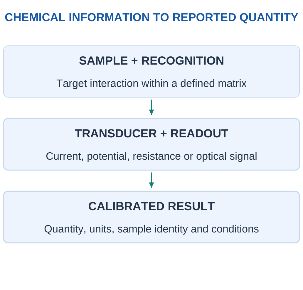
For example, a gas can change the resistance of a metal-oxide surface, an ion can change an electrode potential, or a molecule can absorb selected light. These responses use different mechanisms even when all final readings appear as digital numbers on a screen.
Name the Measurand
A useful result says what quantity is measured: concentration, activity-related pH, gas mole fraction or another defined property. It also needs units, sample identity, time and conditions. “The sensor reads 20” is incomplete without this information.
Key Idea: Recognition Is Not the Transducer
An antibody binding a target supplies a biological recognition event. An attached optical or electrical measurement supplies the reporting signal. Naming the antibody alone does not explain how the result reaches the instrument, and naming a photodiode alone does not establish selective binding.
| Stage | Question to Ask |
|---|---|
| Sample | Which material and location are represented? |
| Interaction | What chemical or physical change occurs? |
| Transducer | What signal changes: current, voltage, light or resistance? |
| Calibration | How is signal related to the requested quantity? |
| Interpretation | What does the result justify under these conditions? |
Sensor Versus Complete Instrument
An active sensing layer is not an entire validated instrument. Packaging, sample access, electronics, compensation and data handling affect the useful result. A chip that detects a response does not automatically identify one substance uniquely in a mixed real sample.
Study Habit
Explain analyte → interaction → signal → calibration → result. Then name a possible interference or failure mechanism. This produces a complete answer rather than a list of sensor names.
Worked Example 3.1: Trace a Defined Chemical Input to a Reported Result
Problem: A supplied sensor model is y = 5 + 2C, with y in mV and C in mg/L. A reference input is 20 mg/L. Find the expected signal and recover C from it. Identify the role of calibration.
Model / Approach: The linear relation is supplied and supported at this input. Background is included in its intercept; no target selectivity, environmental correction or network effect is added to the equation.
Step 1: Target-related signal is mC = 2 × 20 = 40 mV.
Step 2: Total signal is background plus target term = 45 mV.
Step 3: Inverting the same relation gives C = (45 − 5)/2 = 20 mg/L.
Step 4: The calibration connects signal to quantity under its stated conditions. The numerical round trip alone does not validate another chemical mixture or an independent unknown.
Answer: Expected signal = 45 mV; recovered input = 20 mg/L.
Check: A transmitted digital number still needs its units and calibration.
2. Recognition, Adsorption and Transduction
Recognition means a preferential interaction that connects the target chemistry to a measurable change. It may involve surface adsorption, ion exchange, molecular binding, an enzyme reaction or selective absorption of light. Different recognition mechanisms need different operating conditions and verification.

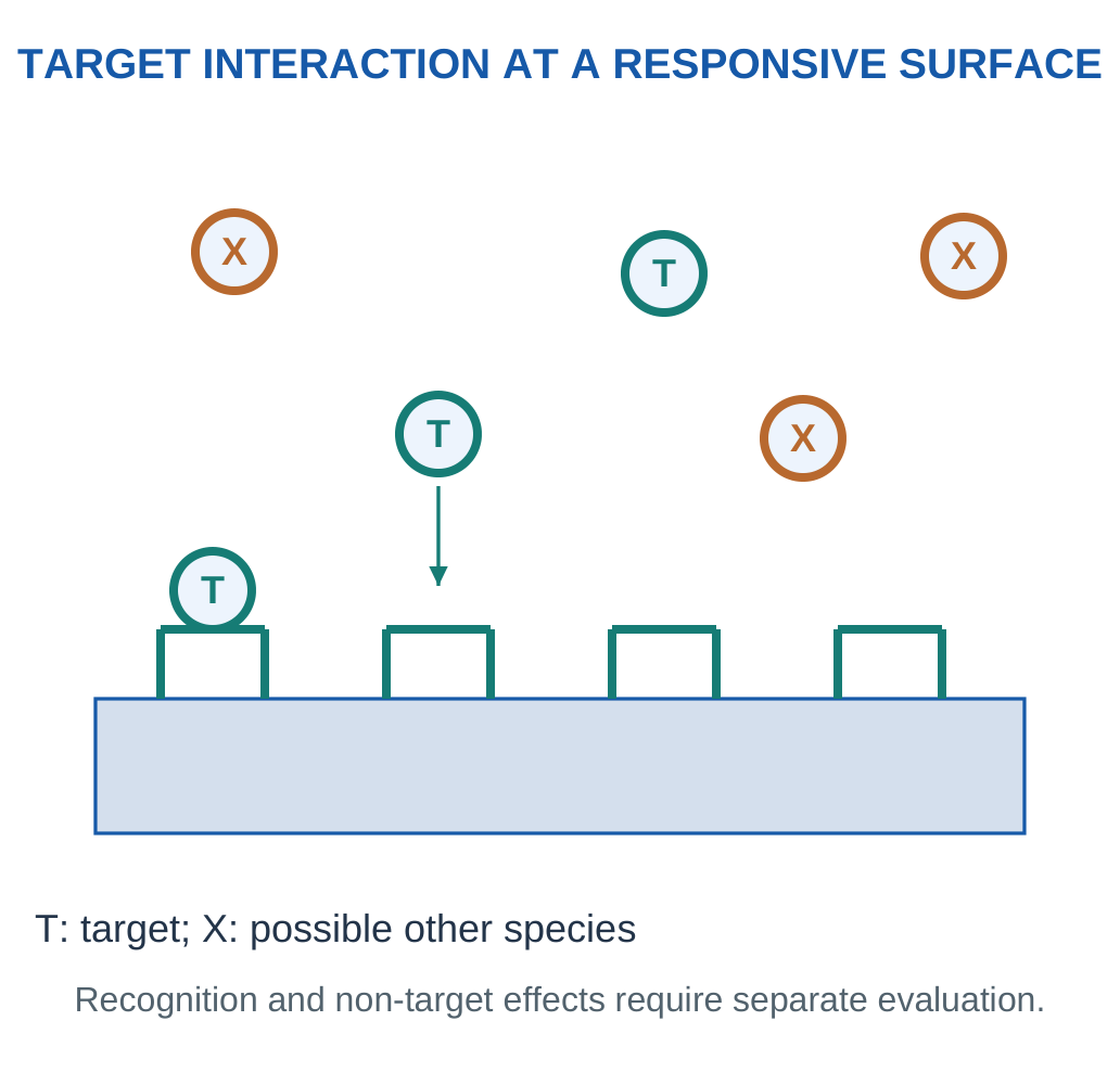
Adsorption is accumulation at an interface, whereas absorption involves entry into a bulk phase. A gas interacting with a porous sensing film can involve both surface and bulk effects, so the mechanism should be identified rather than guessed from the word uptake.
Transduction Families
Electrical resistance changes can arise from surface chemistry or material transport changes. Electrochemical current measures a reaction-related charge-transfer rate under controlled conditions. Electrode potential can reflect an ion-activity-dependent equilibrium response. Optical methods detect absorption, emission or another light-related change.
The recognition layer and the transducer are related but distinct. An antibody can recognise an antigen while an optical or electrical transducer reports the binding. Calling the whole device a biosensor does not by itself identify the signal type.
Reversibility and Access
A useful reusable sensor often needs a response that can recover sufficiently for the next sample. Strong irreversible binding can instead support a single-use assay. Sample diffusion through a membrane, surface fouling and site availability can limit how quickly the chemical interaction occurs.
Distinguish the Words
Sensitive means a response changes with the measurand; selective means other species affect it less under stated conditions. A large signal to many gases is not automatically a selective identification of one gas.
3. Sensitivity, Selectivity, Range and Precision
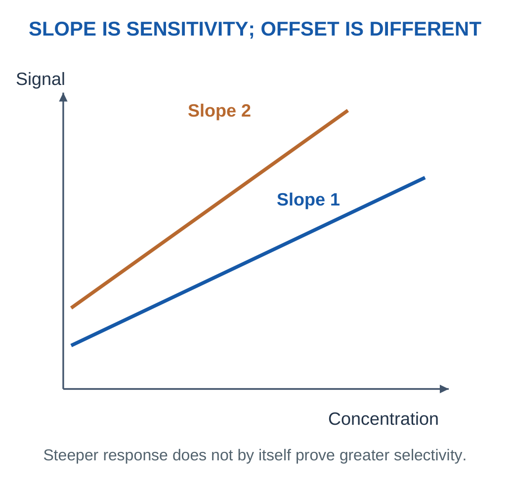
Sensitivity is the local change of signal per change in the input quantity. For a stated linear model y = b + mC, m is the sensitivity in signal units per concentration unit.
Selectivity concerns discrimination against other relevant species or influences; it is not the same as having a steep calibration slope.

Range and Resolution
A calibration has a validated range of input conditions. Extrapolating far beyond it can give an unsupported concentration even if the algebra is easy. Resolution describes the represented signal or input increment. A finer display does not automatically improve accuracy or chemical selectivity.
Bias and Repeatability
Signed error relative to a supplied reference is measured value minus reference. Repeated readings may cluster tightly while their average is offset. That is good repeatability with bias in the comparison. Agreement with a reference and small spread answer different questions.
| Property | What It Describes |
|---|---|
| Sensitivity | Signal change per input change |
| Selectivity | Response relative to interferences |
| Repeatability | Spread under the defined repeated conditions |
| Bias | Average offset relative to a reference |
| Resolution | Smallest represented increment |
| Working range | Conditions over which the model is supported |
Detection Is Not Full Quantification
A signal distinguished from a blank does not automatically provide a precise concentration, identify its chemical origin or demonstrate fitness for a safety/medical application. The relevant noise, calibration, matrix and validation conditions must be stated.
Quick Distinction
A precise instrument can be consistently wrong. A highly sensitive sensor can respond strongly to several substances. A large number of decimal places can still describe a biased measurement.
Worked Example 3.2: Separate Sensitivity from the Zero-Input Offset
Problem: Two supplied points are C = 0 and 20 mg/L, with signals 10 and 50 mV. Assume a linear relation over that interval. Find sensitivity and intercept, and explain which property the slope does not establish.
Model / Approach: Use y = b + mC with the supplied paired data. The model concerns this analyte/condition interval; no interference experiments are supplied to establish selectivity.
Step 1: Input difference is 20 mg/L; signal difference is 40 mV.
Step 2: Sensitivity m = Δy/ΔC = 2 mV per (mg/L).
Step 3: Intercept b = y1 − mC1 = 10 mV.
Step 4: Both points are reproduced by the equation. The slope is analytical sensitivity, not proof that another species has zero response.
Answer: m = 2 mV per (mg/L); b = 10 mV.
Check: A larger intercept is not automatically a larger sensitivity.
Worked Example 3.3: Report Repeated-Measurement Spread and Bias Separately
Problem: Supplied repeated readings are 9.8, 10.0 and 10.2 mg/L under the same conditions. Reference is 10.5 mg/L. Find mean, sample standard deviation using N − 1 and signed mean bias.
Model / Approach: These three readings form only the specified repeated dataset. The reference is supplied as exact for this arithmetic; no broader uncertainty or universal product accuracy is inferred.
Step 1: Mean is sum/N = 10 mg/L.
Step 2: Sum of squared deviations is 0.08 (mg/L)².
Step 3: Sample standard deviation is √[sum/(N − 1)] = 0.2 mg/L.
Step 4: Signed mean bias is mean − reference = −0.5 mg/L. Spread and offset answer different questions even when both are small.
Answer: Mean = 10 mg/L; sample s = 0.2 mg/L; signed bias = −0.5 mg/L.
Check: Do not report the standard deviation as though it were the signed error of the mean.
4. Calibration, Blanks and Sample Preparation
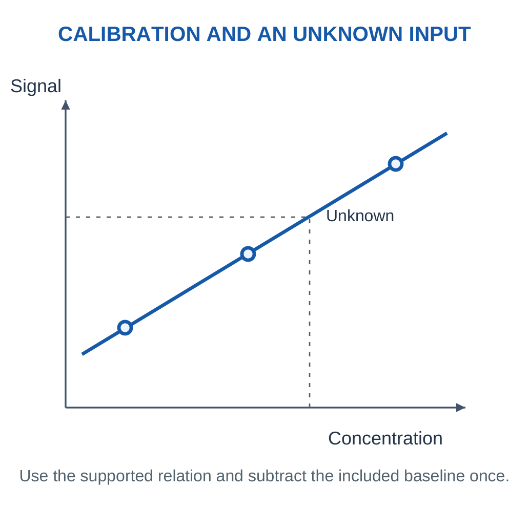
Calibration establishes the relation between a known input and measured signal under stated conditions. A two-point linear model uses:
m = (y2 − y1)/(C2 − C1)
b = y1 − mC1
An unknown input within the supported range is:
C = (y − b)/m

Blank and Background
A blank represents the relevant absence of target under a defined procedure/matrix. Its signal may include electronics offset, solvent/matrix effects or other background. Blank subtraction must be consistent with whether the calibration already contains an intercept; subtracting the same offset twice creates an error.
Dilution
If a sample is diluted by a supplied factor D and its diluted concentration is measured correctly, original concentration is D times that value when the model assumes no loss or reaction and the same quantity definition.
For an ideal volume-based preparation:
C1V1 = C2V2
This applies under the stated final-volume assumptions.
Calibration Versus Validation
A fitted line can match its own standards and still perform poorly on a new sample. Check standards, matrix-matched evaluation and independent reference comparisons provide different evidence. Do not call a high fitted correlation proof that every future mixture is measured correctly.
Sampling Changes Meaning
A filter, inlet tube or extraction step can remove or delay species. The quantity reaching the sensor can differ from that at the original location. A useful reported result states whether it describes the prepared aliquot, diluted solution or original sample.
Calculation Order
Write the signal equation, remove only the included offset once, invert the slope, check the supported range and finally apply any explicitly supplied preparation factor.
Worked Example 3.4: Infer a Calibrated Concentration and Original-Sample Basis
Problem: A supplied linear calibration has (0 mg/L, 5 mV) and (10 mg/L, 45 mV). A prepared sample gives 29 mV and its original-to-measured concentration dilution factor is 1. Find measured and original concentrations.
Model / Approach: Assume no preparation loss/reaction and a supported linear interval. Dilution factor refers to original concentration divided by prepared concentration; background is included once in the fitted intercept.
Step 1: Slope is 4 mV per (mg/L); intercept is 5 mV.
Step 2: Prepared concentration is (signal − intercept)/slope = 6 mg/L.
Step 3: This lies within the stated calibration interval. Original concentration is D × prepared = 6 mg/L.
Step 4: Substituting the prepared result back into y = b + mC gives 29 mV. Dilution changes the reported sample basis, not the original calibration slope.
Answer: Prepared = 6 mg/L; original = 6 mg/L.
Check: Subtracting the blank again after using the intercept would double-correct background.
Worked Example 3.5: Use a Stated Ideal Dilution Mass Balance
Problem: An aliquot 5 mL at 100 mg/L is diluted to a defined final volume 50 mL. Assume no target loss or reaction and the stated final-volume model. Find diluted concentration and factor.
Model / Approach: Use CinitialValiquot = CfinalVfinal with matching volume units. The final volume is supplied; it is not inferred by adding arbitrary non-additive solvent volumes.
Step 1: The concentration-volume balance gives Cfinal = 100 × 5/50.
Step 2: Diluted concentration is 10 mg/L.
Step 3: Dilution factor D = final/aliquot = 10.
Step 4: Cfinal × D = 100 mg/L recovers the original concentration. A sensor result must be labelled before or after this correction.
Answer: Diluted concentration = 10 mg/L; D = 10.
Check: A preparation factor assumes the target is preserved.
5. Noise, Drift and Response-Time Models
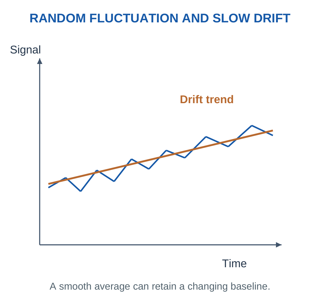
Noise describes unwanted fluctuations over the specified observation conditions. Drift is a slower change in response with time or exposure. A sensor can have low short-term noise but a changing baseline or sensitivity. Averaging may reduce some random noise while leaving drift and systematic interference largely unchanged.

A Conditional Detection Estimate
An introductory blank-noise estimate may define concentration threshold as:
3σblank/|m|
Here m is the linear sensitivity and σblank is the signal standard deviation. This convention requires the supplied noise and model assumptions. It is not a universal guarantee of detection probability, selectivity or a complete validated detection limit for every method.
Response and Recovery
Response time measures how quickly a defined fraction of a final response is reached after a stated input change. Recovery concerns return toward a specified baseline after removal/change of input. State the fraction and endpoints; t90 and t63 do not represent the same point.
For a supplied first-order model:
Fraction Reached = 1 − exp(−t/τ)
Therefore:
t90 = τ ln 10
Sample transport delay, mixing and surface kinetics can contribute additional behaviour. A short electronics sampling interval is not automatically the chemical response time.
Practical Meaning
A drifting baseline can imitate a concentration change. Fouling or poisoning can change slope or recovery. Periodic checks should match the relevant property rather than correcting every problem with a single fixed offset.
Do Not Overclaim
A calculated noise threshold concerns the specified signal model. A fast sample clock or small standard deviation alone cannot establish chemical identification, long-term stability or suitability for a critical application.
Worked Example 3.6: Evaluate a Supplied Blank-Noise Threshold Convention
Problem: Blank signal standard deviation is 0.2 mV and linear sensitivity magnitude 2 mV per (mg/L). The exercise defines its concentration threshold as 3σblank/|m|. Calculate that estimate and its meaning.
Model / Approach: Use the explicitly stated convention. No universal detection probability, chemical selectivity or complete validated limit of detection is inferred from this simplified noise/linearity model.
Step 1: Three times the blank standard deviation is 0.6 mV.
Step 2: Divide by sensitivity magnitude: threshold = 0.6/2 = 0.3 mg/L.
Step 3: Multiplying the concentration estimate by |m| recovers the 3σ signal increment.
Step 4: The estimate addresses signal-to-blank separation under the given conditions. Quantification, interferences and another sensor state need their own evaluation.
Answer: Supplied-convention threshold = 0.3 mg/L.
Check: A threshold estimate is not the same as the lowest printed standard, display resolution or a guarantee that any signal above it identifies the intended analyte.
Worked Example 3.7: Combine a Supplied Fixed Delay with One Response Stage
Problem: A model has fixed sample delay 2 s followed by a first-order sensor with τ = 5 s and fraction reached 1 − exp(−t/τ) after arrival. Find total time from the original step to 90% response.
Model / Approach: Only one exponential stage follows the given pure delay. The stage clock starts after sample arrival; no additional mixing, adsorption or electronics filtering is included.
Step 1: Required remaining fraction is 1 − 0.9 = 0.1.
Step 2: Exponential-stage time is −τ ln(1 − fraction) ≈ 11.5129 s.
Step 3: Total time from the original change is delay + stage time ≈ 13.5129 s.
Step 4: Using the stage time in 1 − exp(−t/τ) gives 0.9. Sampling more frequently does not remove the supplied physical delay.
Answer: Stage time ≈ 11.5129 s; total time ≈ 13.5129 s.
Check: Do not insert the total time including delay into the exponential that is defined only after arrival.
6. Electrochemical Sensors and Electrode Roles
An electrochemical sensor connects chemical processes at interfaces with an electrical measurement. Important modes include amperometry, which measures current at a controlled potential, and potentiometry, which measures an electrode-potential difference under a high-impedance, near-zero-current condition.
Key Idea: Reference and Counter Are Different Functions
The reference supports the potential comparison with very small sensing current. The counter carries the main cell current in the stated three-electrode arrangement. Routing the analytical current through the ideal reference input would defeat the reason for separating these roles.

What to Notice
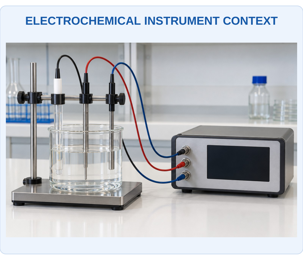
Electrodes and cables provide different sensing and current functions. The exact diagram below identifies working, reference and counter roles; the equipment appearance alone cannot establish which lead performs which function or what chemical signal is being measured.

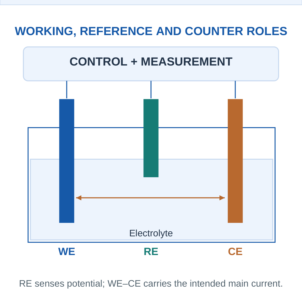
The working electrode is the interface of analytical interest.
The reference electrode provides a suitably stable comparison potential.
The counter/auxiliary electrode completes the main current path in a three-electrode controlled-potential arrangement.
Why Separate the Reference Path?
A reference that carries substantial cell current can become polarised and shift the comparison potential. A suitable high-impedance measurement path draws negligible current relative to the intended main path. This is a functional idealisation; real electrodes and electronics have limitations.
Electrolyte and Sample
The electrolyte supplies ionic continuity. Surface condition, reaction kinetics, transport and sample composition influence the signal. The current in a metal lead and ion transport through a liquid complete a circuit through different carriers; they are not the same electrons flowing through all regions unchanged.
Not Every Sensor Needs Three Exposed Electrodes
Configurations depend on the technique and integrated design. A potentiometric ion-selective measurement may use an indicator and reference arrangement; some amperometric devices integrate reference/counter functions differently. Explain the stated configuration rather than imposing one drawing universally.
Diagram Rule
Label the electrode functions before drawing current and voltage paths. Do not route the main amperometric current through the ideal reference-sensing input.
7. Amperometric Sensing: Current at Controlled Potential
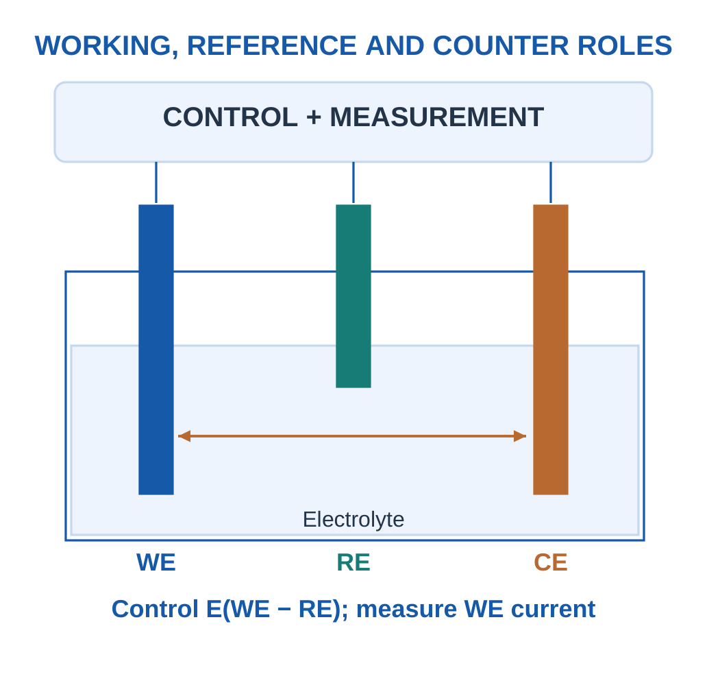
In amperometry, the working-electrode potential is controlled relative to a reference and the resulting current is measured. A relevant analyte or reaction product undergoes oxidation/reduction in the selected potential region. Under appropriate transport and reaction conditions, the current can be related to analyte concentration.

What Determines Current?
Current reflects charge-transfer rate. If a reaction transfers z electrons per molecule and the assigned reacted amount rate is r mol/s:
I = zFr
This applies for full assigned efficiency. A supplied collection/current efficiency modifies the relevant rate contribution. This balance does not prove that every molecule in a flowing sample reacts.
The measured signal can also depend on diffusion, convection, electrode area, temperature, fouling and competing electroactive species. A simple I = Iblank + kC model is useful only over its stated range and conditions.
Examples and Limits
Electroactive gases or enzyme-generated species can support amperometric detection. A sensor measuring hydrogen peroxide from an enzyme reaction does not directly count every glucose molecule independently of reaction/transport limitations. The chemical coupling and calibration must both be explained.
Current Sign
Oxidation and reduction currents can be assigned opposite signs by the instrument convention. A magnitude-based calibration must state that convention or use the signed equation supplied. “Larger absolute current” does not necessarily mean the same direction of reaction in every sensor.
Memory Cue
Amperometry: control potential, measure current.
Potentiometry: measure potential difference with negligible current.
Keep the controlled and observed quantities separate.
Worked Example 3.8: Convert an Assigned Reaction Rate into Current
Problem: The supplied analyte reaction transfers 2 electrons per molecule, with target molar arrival/reaction basis 2 × 10⁻¹⁰ mol/s and assigned current-collection fraction 1. Use F = 96485 C/mol. Find the target current magnitude.
Model / Approach: Use I = zF × rate × assigned fraction. The supplied fraction defines the collected analytical share; the model does not claim every molecule in an actual flowing sample reacts or that interference current is absent unless stated.
Step 1: Assigned collected reaction amount rate is 2 × 10⁻¹⁰ mol/s.
Step 2: Electron amount rate is z times this = 4 × 10⁻¹⁰ mol electrons/s.
Step 3: Current is F times electron amount rate = 3.8594 × 10⁻⁵ A = 38.594 µA.
Step 4: Dividing by zF recovers the collected reaction rate, checking stoichiometry and charge-per-time units.
Answer: Target current magnitude = 38.594 µA.
Check: Faraday balance converts assigned reaction rate to current; calibration and sample transport determine whether that assigned rate represents the original analyte concentration.
8. Amperometric Calibration and Interferences
A supplied linear amperometric calibration may be:
I = I0 + kC
I0 is the stated baseline and k the sensitivity. Inverting gives:
C = (I − I0)/k
The units of current and concentration must match those used to define k; mixing µA and nA changes the result by 1000.


More Than One Responding Species
If a second electroactive species contributes a current, one scalar reading may not uniquely determine the target concentration without additional information.
A supplied linear example can write:
I = I0 + kACA + kBCB
Neglecting B generally biases an estimate of A unless its effect is known to be negligible.
Selective Potential and Membranes
Choice of potential or a selective transport layer can reduce some interferences, but no generic diagram proves perfect selectivity. A membrane may also slow transport or change sensitivity. Surface modification can improve one property while introducing a different environmental or ageing dependence.
Check a Known Sample
A check solution or independent comparison can reveal a changed baseline/slope. A zero-only correction repairs an additive offset in a supplied model; it cannot automatically repair a changed sensitivity. A two-point check can distinguish these simple changes more effectively.
Report the Limit
A concentration obtained from a mixed-signal equation is conditional on the supplied interference model. The presence of a clean electrical trace does not establish that the current came only from the intended chemistry.
Solving Sequence
Convert current units, define the baseline, identify any supplied interference term, subtract each once and divide by the appropriate target sensitivity. Then check the range and assumptions.
Worked Example 3.9: Invert a Supplied Current Calibration
Problem: A supplied model is I = 0.5 + 2C, with I in µA and C in mg/L. Prepared-sample current is 8.5 µA. Original concentration is defined as 1 times prepared concentration. Calculate both concentrations.
Model / Approach: The baseline and slope are supplied for this supported condition. No independent interference term is present in this exercise; do not subtract an extra blank after already using the intercept.
Step 1: Target-related current is I − I0 = 8 µA.
Step 2: Prepared concentration is 8/2 = 4 mg/L.
Step 3: Original-basis concentration is D × prepared = 4 mg/L.
Step 4: Back-substitution produces 8.5 µA. The current units must match the sensitivity’s µA unit before inversion.
Answer: Prepared = 4 mg/L; original = 4 mg/L.
Check: An amplifier output or a current reading does not itself prove target selectivity.
Worked Example 3.10: Remove an Independently Supplied Interference Term
Problem: A model gives I = I0 + kACA + kBCB in µA. I0 = 0.2 µA, kA = 2 and kB = 0.5 µA per (mg/L). Target A is 4 mg/L and B is independently known as 3 mg/L. Calculate total current and the A estimate with and without B correction.
Model / Approach: The contributions are explicitly additive and B concentration is independently supplied. A single mixed current without that extra information would not uniquely determine both unknown concentrations.
Step 1: Total I = 0.2 + 2 × 4 + 0.5 × 3 = 9.7 µA.
Step 2: Ignoring B gives apparent A = (I − I0)/kA = 4.75 mg/L.
Step 3: Subtracting the known B term gives corrected A = 4 mg/L.
Step 4: The uncorrected positive bias is 0.75 mg/L. The correction is justified only by the supplied additive interference relation and known B.
Answer: Total = 9.7 µA; uncorrected A = 4.75 mg/L; corrected A = 4 mg/L.
Check: A current signal may contain several chemical contributions.
9. Potentiometric Sensing and Ion Activity
Potentiometry measures a potential difference between an indicator and a suitable reference electrode with very small macroscopic current in the intended measurement. An ion-selective membrane/electrode can have an activity-dependent response rather than a current directly proportional to concentration.

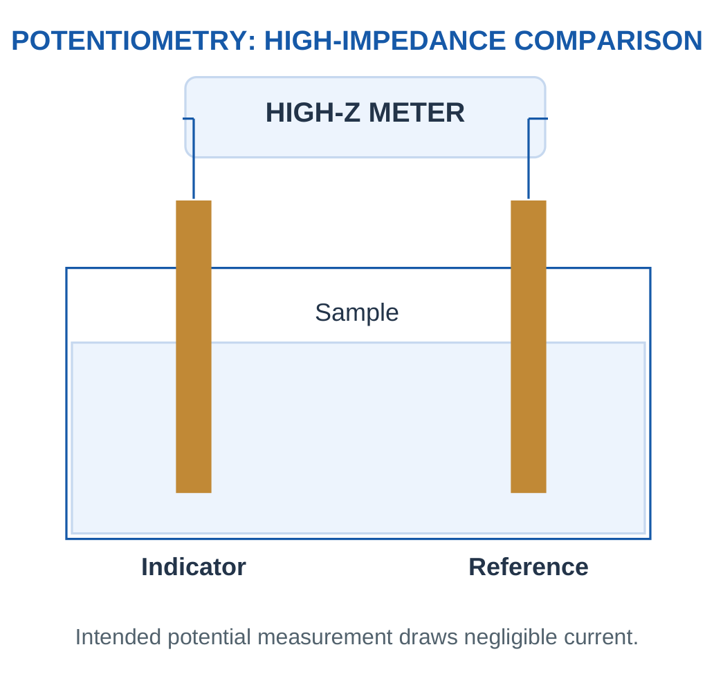
For a supplied ideal cation response:
E = E0 + (RT/zF) ln a
A 298 K base-10 model uses:
E = E0 + (59.16/z)log10 a
Here E is in mV. The activity a is dimensionless relative to the stated standard; concentration can replace it only under an explicitly supplied approximation.
Charge Sign and Slope
The sign of z matters in a general ion response. These introductory examples specify a cation or give a signed calibrated slope to avoid an unqualified rule that every ion sensor’s potential increases with concentration. The reference and measured cell orientation can also affect the written intercept/sign convention.
Activity Is Not Simply Amount
Activity reflects effective chemical behaviour in the stated thermodynamic model. Two solutions with equal analytical concentration can have different activity when their environments differ. A calibration made in an appropriate matrix or with an activity treatment helps connect the response to the requested quantity.
Useful Distinctions
The near-zero-current measurement does not mean the electrode has no chemical interaction. Equilibrium/interfacial processes create the measured potential. Conversely, forcing substantial current can disturb that intended potential and change the measurement mode.
Remember
Use the complete signed equation and its reference convention. A millivolt value without a reference, temperature and calibration cannot uniquely identify an ion concentration.
Worked Example 3.11: Use a Defined Ideal Monovalent Cation Activity Response
Problem: At the supplied 298 K approximation, a cation sensor follows E = 200 + (59.16/1)log10 a in mV, with dimensionless activity a = 0.01. Find potential and recover activity from it.
Model / Approach: The reference orientation and intercept are defined by the equation. Use activity as supplied, not an unqualified concentration substitution; no substantial measurement current is assumed.
Step 1: log10 a = −2.
Step 2: Potential correction is (59.16/1)log10 a = −118.32 mV.
Step 3: E = 81.68 mV; inversion gives a = 10^[z(E − E0)/59.16] = 0.01.
Step 4: The slope magnitude per decade is 59.16 mV. It depends on the specified charge magnitude and temperature model.
Answer: E = 81.68 mV; recovered a = 0.01.
Check: Use the signed equation actually supplied.
Worked Example 3.12: Use a Defined Ideal Divalent Cation Activity Response
Problem: At the supplied 298 K approximation, a cation sensor follows E = 100 + (59.16/2)log10 a in mV, with dimensionless activity a = 0.001. Find potential and recover activity from it.
Model / Approach: The reference orientation and intercept are defined by the equation. Use activity as supplied, not an unqualified concentration substitution; no substantial measurement current is assumed.
Step 1: log10 a = −3.
Step 2: Potential correction is (59.16/2)log10 a = −88.74 mV.
Step 3: E = 11.26 mV; inversion gives a = 10^[z(E − E0)/59.16] = 0.001.
Step 4: The slope magnitude per decade is 29.58 mV. It depends on the specified charge magnitude and temperature model.
Answer: E = 11.26 mV; recovered a = 0.001.
Check: Use the signed equation actually supplied.
10. pH Electrodes and Two-Point Calibration
pH is defined through hydrogen-ion activity:
pH = −log10 aH+
In a simplified dilute-solution example, the activity may be approximated using the supplied concentration convention. pH is logarithmic; a one-unit change corresponds to a factor of ten in hydrogen-ion activity.

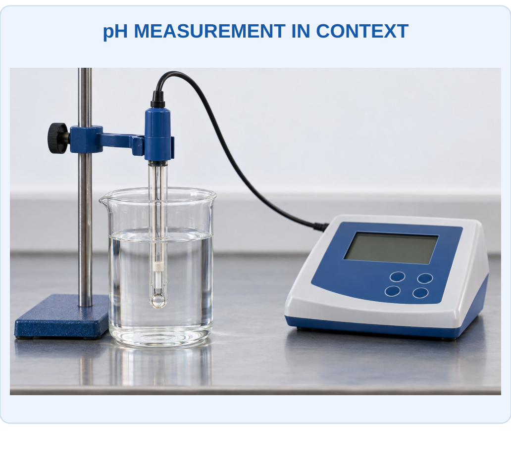
What to Notice
The wetted sensing region and reference contact must interact with the same represented sample. A displayed pH needs appropriate calibration and temperature context. The glass bulb is an ion-responsive interface, not a metal conductor for ordinary external electron flow.

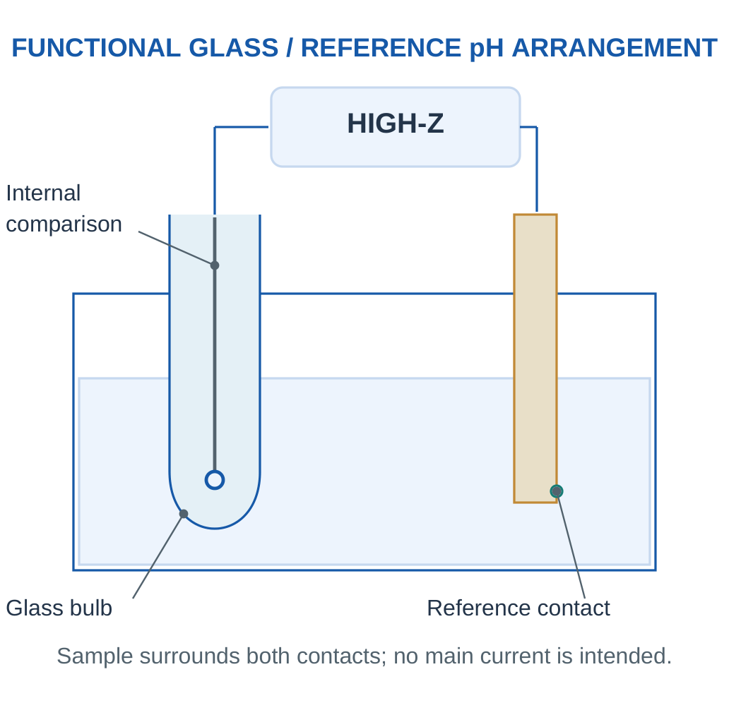
A supplied electrode model can be:
E = E0 − S pH
S is a positive slope magnitude at the stated temperature and meter convention. The ideal monovalent slope magnitude near 298 K is about 59.16 mV per pH unit, but actual calibration and temperature must be used rather than treating one value as universal.
Why Calibrate at Two Points?
Two defined buffer readings estimate both slope and intercept. A single-point check can identify an offset at that point without proving the sensitivity is correct elsewhere. Calibration should be interpreted in its temperature and range rather than extrapolated indefinitely.
Glass and Reference Functions
The hydrated glass surface supports a hydrogen-ion-responsive potential through appropriate ion interactions. The reference provides a stable comparison and an ionic contact with the sample. The measurement is not explained by ordinary free electrons passing directly through the glass bulb as if it were copper.
Handling as a Concept
Hydration, surface contamination, junction condition and temperature affect response. The actual probe’s supported care and calibration procedure governs use. These notes explain the functions without replacing that specific instrument guidance.
pH Trap
The average of two pH numbers is not generally the pH of physically mixed solutions. Mixing requires chemical amounts, volumes and equilibria; the logarithmic scale cannot be averaged as an automatic mixing law.
Worked Example 3.13: Two-Point pH Calibration Including a Real Supplied Slope
Problem: A supplied electrode reads 170 mV at pH 4 and −7 mV at pH 7. Assume a linear potential-pH relation between these points at fixed conditions. Unknown signal is 52 mV. Find slope, intercept and pH.
Model / Approach: Use E = b + mpH fitted to the supplied buffers. Do not replace the measured slope with an ideal textbook value. The unknown is interpreted only within the supported interval and conditions.
Step 1: Slope m = (−7 − 170)/(7 − 4) = −59 mV per pH.
Step 2: Intercept b = 170 − (−59 × 4) = 406 mV.
Step 3: Unknown pH = (E − b)/m = 6.
Step 4: Back-substitution returns 52 mV. The negative slope follows this supplied electrode/meter convention.
Answer: m = −59 mV/pH; b = 406 mV; unknown pH = 6.
Check: A zero correction alone cannot replace the two-point slope information. pH is dimensionless and logarithmic, not a concentration in mg/L.
Worked Example 3.14: Compare Hydrogen-Ion Activities on the Logarithmic Scale
Problem: Two ideal model samples have pH 5 and 7. Use pH = −log10 aH+. Calculate both activities and the ratio first/second. Do not physically mix the samples.
Model / Approach: Activities are dimensionless as defined. The exercise compares two separate values and supplies no acid/base composition or volume information for a mixing calculation.
Step 1: First activity is 10^(−5) = 1 × 10⁻⁵.
Step 2: Second is 10^(−7) = 1 × 10⁻⁷.
Step 3: Ratio first/second = 10^(7 − 5) = 100.
Step 4: The lower pH has greater hydrogen-ion activity. This does not mean the pH difference is an additive molar concentration or that their average predicts a mixture.
Answer: Activities = 1 × 10⁻⁵ and 1 × 10⁻⁷; ratio = 100.
Check: Preserve the logarithmic definition.
11. Comparing Electrochemical Sensing Modes
Amperometric and potentiometric modes both involve electrodes but answer through different observables. Amperometry measures reaction-related current at a controlled potential. Potentiometry measures an indicator/reference potential difference under a high-impedance condition.


| Feature | Amperometric Model | Potentiometric Model |
|---|---|---|
| Main measured quantity | Current | Potential difference |
| Control/condition | Defined working potential | Very small measurement current |
| Typical relation | Calibrated current versus target | Activity/logarithmic potential response |
| Key concerns | Transport, competing reactions, fouling | Reference stability, activity, membrane response |
Conductivity as a Related Distinction
A conductivity measurement responds to charge transport by ions in a solution and is not automatically selective for one chemical species. It differs from an ion-selective activity response and from target reaction current. A high ionic conductivity could result from several possible compositions.
Choosing for a Task
Identify whether the target can participate in the intended electrochemical reaction or membrane response, the sample matrix, required range and interfering species. Then evaluate response time, drift and calibration. A current output is not inherently better than a voltage output; chemical suitability and evidence determine the useful choice.
Examination Method
Write one sentence for principle, name the electrode functions, give the relevant signal relation and explain one important limitation. A comparison table is strongest when it compares the same property across both modes.
12. Gas Sensing and Concentration Conventions
A gas sensor must bring a representative gas sample to an active region. Diffusion, flow, inlet volume, adsorption on tubing and environmental conditions can alter the concentration and timing at the sensing surface. The first detected response therefore need not occur at the exact time the original environment changed.
Key Idea: Conductivity Does Not Identify One Ion
A solution can carry ionic current because several dissolved species contribute. A conductivity value therefore differs from a selective ion-activity or target-reaction measurement. The sensor mode must match the requested chemical quantity rather than only the presence of an electrical output.
Key Idea: State the Oxide Response Direction Conditionally
A common n-type reducing-gas example can show falling resistance through the supplied surface/carrier mechanism. Another oxide, oxidising gas or operating environment can differ. The observed sign must be linked to the stated material and conditions rather than a universal pollutant rule.


ppm and ppb
For an explicitly stated gas mole-fraction basis, 1 ppm means 10⁻⁶ and 1 ppb means 10⁻⁹ of the total molar amount.
1 ppm = 1000 ppb
These dimensionless fraction conventions should not be silently exchanged with mass concentration in mg/m³.
For an ideal-gas approximation at a specified temperature and pressure, mass concentration can be related to mole fraction using the gas molar volume. A supplied 24.45 L/mol approximation corresponds to about 25°C and one atmosphere; it is not a universal factor at all conditions.
Concentration Versus Exposure
An instantaneous reading, a time average and an integrated concentration-time quantity are different results. Their usefulness depends on the stated question and data coverage. No generic sensor reading alone establishes a medical interpretation or a regulatory compliance conclusion.
A Mixed Environment
Humidity, oxygen content, temperature and background gases can influence different sensing mechanisms. A calibration in one gas composition may not remain exact in another. A sensor’s target label does not prove that all other species are invisible.
Unit Habit
Write ppmv/mole fraction when that is the supplied basis, state temperature/pressure for mass conversion and preserve the sample location/time definition when comparing measurements.
Worked Example 3.15: Convert a Supplied Gas Mole Fraction to Mass Concentration
Problem: A gas has 10 ppm on the stated ideal mole-fraction basis. Its molar mass is 44 g/mol and the supplied gas molar volume is 24.45 L/mol at about 25°C and one atmosphere. Find fraction, ppb and mg/m³.
Model / Approach: Use the explicitly supplied ideal-gas state conversion:
mg/m³ = ppm × M/Vm
This factor is not assumed unchanged at other temperature/pressure conditions or on a different ppm basis.
Step 1: Mole fraction is ppm × 10⁻⁶ = 1 × 10⁻⁵.
Step 2: Equivalent ppb is ppm × 1000 = 10000.
Step 3: Mass concentration is 10 × 44/24.45 ≈ 17.9959 mg/m³.
Step 4: Inverse ppm = (mg/m³)Vm/M gives 10. The molar mass makes equal ppm values correspond to different mass concentrations for different gases.
Answer: Fraction = 1 × 10⁻⁵; 10000 ppb; approximately 17.9959 mg/m³ at the stated state.
Check: Do not equate ppm directly with mg/m³.
13. Metal-Oxide Gas Sensors: Surface Chemistry
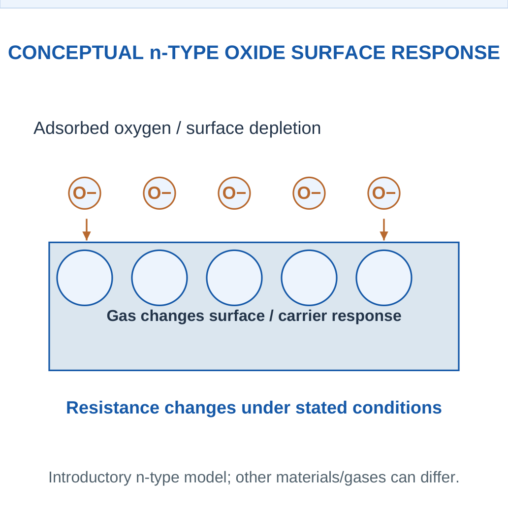
Metal-oxide gas sensors use a gas-dependent electrical response of a semiconducting oxide. A common introductory n-type SnO2 model involves surface oxygen interactions that withdraw electronic carriers and alter the near-surface conduction barrier. Exposure to an appropriate reducing gas can change these surface species and return carriers, lowering resistance under the stated conditions.

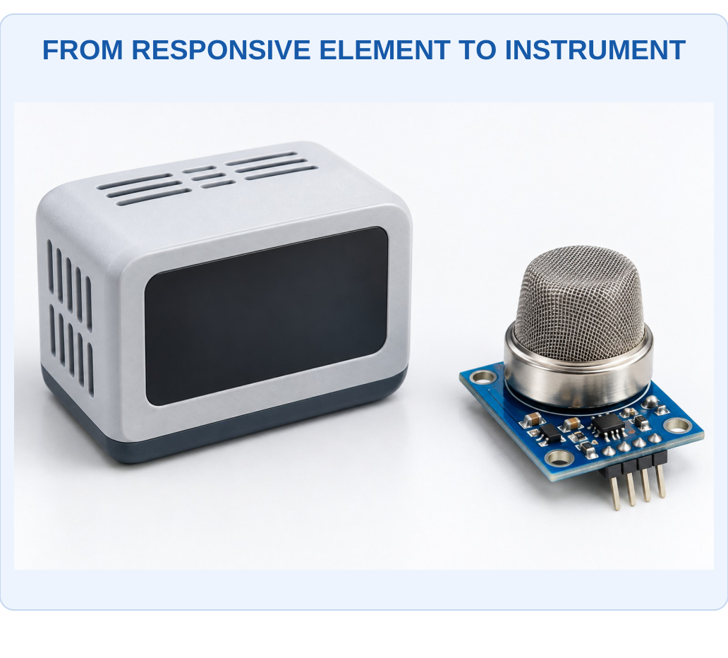
What to Notice
A component requires an appropriate sample path, readout and calibrated interpretation. Its mesh, enclosure or display does not prove selective measurement of one gas. The material mechanism and interference evaluation determine what the complete instrument can justify.

Heating and Surface State
Many such sensing elements operate with a controlled heated active region. Temperature affects adsorption, reaction and desorption as well as electrical transport. A small heater does not make its setpoint a measure of ambient air temperature or identify gas concentration by itself.
Direction Is Conditional
The familiar reducing-gas resistance decrease belongs to the stated n-type mechanism and conditions. Other oxide types, oxidising gases and operating regimes can give different responses. Do not write that every metal-oxide sensor’s resistance always falls for every pollutant.
Real Selectivity
Different gases can produce overlapping responses. Water and background oxygen can also change behaviour. Material composition, catalysts, microstructure and temperature operation influence useful response, but a single resistance change is not necessarily a unique chemical identification.
Applications
Suitable devices can support air-quality and process-sensing tasks within their calibrated range and environment. Critical alarm suitability requires the relevant approved complete instrument rather than a generic semiconductor resistance experiment.
Connect the Chain
Gas/surface interaction → carrier/barrier change → resistance change → calibrated signal.
The heater, sensing resistance and readout voltage are separate quantities.
Worked Example 3.16: Keep Response-Ratio Definitions Distinct
Problem: A supplied oxide-sensor example has baseline resistance 100 kΩ and exposed resistance 40 kΩ. Calculate Rgas/Rair, Rair/Rgas and (Rgas − Rair)/Rair. Explain whether all three can be called the same number.
Model / Approach: Only the defined resistance comparison is calculated. The definitions also allow an increasing resistance in another case; no universal gas identity or oxide mechanism is inferred from the sign alone.
Step 1: Rgas/Rair = 40/100 = 0.4.
Step 2: Rair/Rgas = 100/40 = 2.5.
Step 3: Normalised change is (40 − 100)/100 = −0.6, or −60%.
Step 4: The first two are reciprocals and the third is a signed relative change. Their differing definitions must be preserved when reading a calibration.
Answer: Ratios = 0.4 and 2.5; normalised change = −0.6.
Check: A resistance sign cannot uniquely establish gas identity or prove every metal oxide responds in the same direction.
Worked Example 3.17: Compare a Second Resistance Pair
Problem: A supplied oxide-sensor example has baseline resistance 80 kΩ and exposed resistance 20 kΩ. Calculate Rgas/Rair, Rair/Rgas and (Rgas − Rair)/Rair. Explain whether all three can be called the same number.
Model / Approach: Only the defined resistance comparison is calculated. The definitions also allow an increasing resistance in another case; no universal gas identity or oxide mechanism is inferred from the sign alone.
Step 1: Rgas/Rair = 20/80 = 0.25.
Step 2: Rair/Rgas = 80/20 = 4.
Step 3: Normalised change is (20 − 80)/80 = −0.75, or −75%.
Step 4: The first two are reciprocals and the third is a signed relative change. Their differing definitions must be preserved when reading a calibration.
Answer: Ratios = 0.25 and 4; normalised change = −0.75.
Check: A resistance sign cannot uniquely establish gas identity or prove every metal oxide responds in the same direction.
14. Metal-Oxide Readout and Cross-Sensitivity
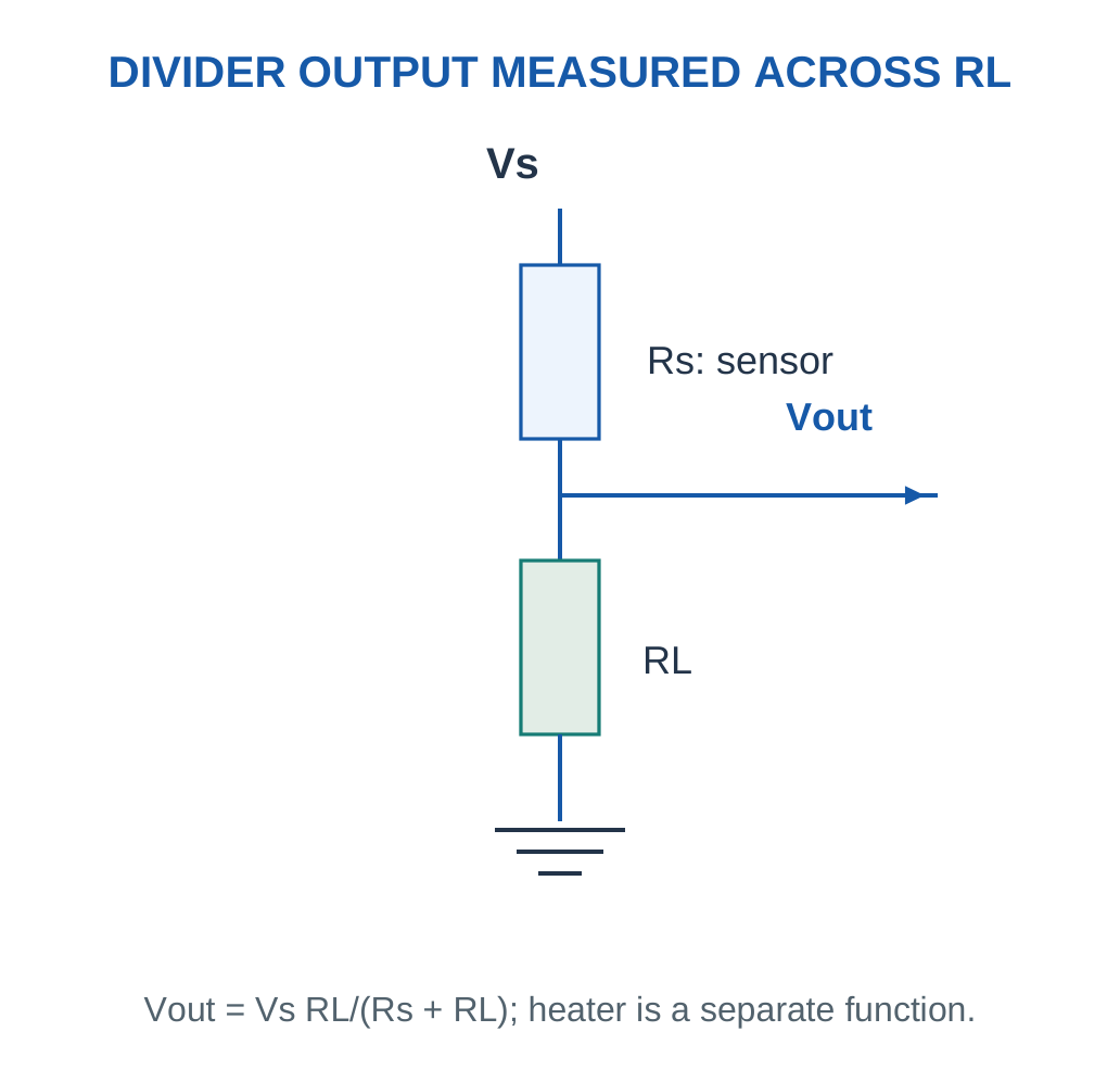
A sensing resistance may be read through a supplied divider or other circuit. For a divider with sensor Rs above a load resistor RL to ground, the voltage across RL is:
Vout = VsRL/(Rs + RL)
If Rs decreases while Vs and RL remain fixed, this defined Vout increases. Measuring across Rs instead gives a different relation.
Key Idea: Optical Path Belongs to the Measured Beam
The path l is the length travelled through the absorbing sample in the supplied model. It is not automatically the outside width or volume label of a container. A changed path must be reflected in the calibration before comparing inferred concentrations.

Define the Response Ratio
A problem may use Rgas/Rair, Rair/Rgas or (Rgas − Rair)/Rair. These definitions can produce different magnitudes and signs for the same resistance pair. Always copy the stated definition before interpreting the result.
Calibration Is Often Nonlinear
A supplied empirical power relation can connect response ratio and concentration over a stated interval. It is not derived by the divider formula alone. A divider converts resistance to voltage; chemistry and calibration determine what that resistance means.
Interference and Drift
A baseline can change with humidity, temperature, contamination or material ageing. A one-point offset cannot automatically correct a changing chemical sensitivity or nonlinear response. Recalibration needs known conditions and suitable validation rather than arbitrary adjustment until a desired number appears.
Calculation Order
Identify the measured resistor, solve the electrical conversion, then apply the separately supplied concentration model. A correct divider voltage does not itself establish selectivity or the true target concentration in a mixture.
Worked Example 3.18: Calculate Voltage Across the Specified Divider Resistor
Problem: A paper divider has Vs = 5 V, upper sensor Rs = 30 kΩ and lower RL = 10 kΩ to ground. Output is across RL. Find output and recover Rs from that voltage.
Model / Approach: Use Vout = VsRL/(Rs + RL), with negligible meter loading and matching resistance units. The separate heater function is not part of this simplified divider.
Step 1: Resistance fraction across RL is 10/(30 + 10) = 0.25.
Step 2: Output is 5 times that fraction = 1.25 V.
Step 3: Rearrange Rs = RL(Vs/Vout − 1) to obtain 30 kΩ.
Step 4: The recovered resistance matches the supplied value. A chemical calibration is still needed to turn resistance into target concentration.
Answer: Vout = 1.25 V; recovered Rs = 30 kΩ.
Check: Measuring across Rs instead would use a different numerator.
15. Optical Chemical Sensing and Beer–Lambert Law
Optical sensors connect chemical information to absorption, emission, colour, refractive behaviour or another light-related property.
In a supplied uniform absorption model:
T = I/I0
A = log10(I0/I) = −log10 T
The incident/reference intensity must correspond to the appropriate blank and optical arrangement.
Key Idea: A Reference Channel Has a Defined Correction Role
If both channels are scaled equally by a supplied common source factor, their ratio can remain unchanged. A deposit that affects only the target band may not cancel. The ratio model does not justify calling every optical or chemical interference corrected.


What to Notice
The beam must traverse the specified sample length through suitable optical faces. Bubbles, contamination, scattering and changing species can disturb the simple absorption model. A coloured solution is not a measured absorbance until the reference and detector conditions are defined.

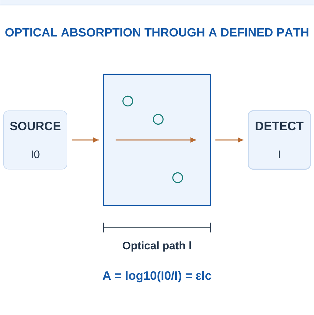
For a stated Beer–Lambert model:
A = εlc
Here ε is the molar absorptivity at the specified wavelength, l path length and c concentration in matching units. The relation assumes the supplied homogeneous sample and appropriate optical/chemical conditions.
Absorbance Is Logarithmic
A = 1 corresponds to T = 0.1; A = 2 corresponds to T = 0.01. Doubling absorbance does not halve transmitted intensity. Absorbance is dimensionless, even though ε carries reciprocal concentration-length units.
Why Conditions Matter
Scattering, stray light, changing chemical species, instrument offset and excessive absorption can violate the simple concentration relation. A coloured sample does not automatically obey one linear calibration at every concentration or wavelength.
Emission Differs from Absorption
A fluorescent response can involve excitation at one wavelength and measured emission at another. Quenching or background fluorescence can affect that signal. A fluorescence intensity calibration is not automatically the same equation as Beer–Lambert absorbance.
Solve Consistently
Correct the defined background first, calculate the proper intensity ratio, take the specified logarithm and use the matching ε, l and concentration units. Do not insert percent transmittance as though it were a fraction.
Worked Example 3.19: Convert Intensity Ratio, Transmission and Absorbance
Problem: A supplied blank/reference intensity is 100 units and transmitted sample intensity 50 units after all stated background handling. Calculate transmittance, percent transmittance and absorbance.
Model / Approach: Use T = I/I0 and A = −log10 T. Both intensities are comparable on the defined optical scale. No scattering or stray-light correction is invented beyond the given model.
Step 1: Transmittance fraction T = 50/100 = 0.5.
Step 2: Percent transmission is 100T = 50%.
Step 3: Absorbance A = −log10(0.5) ≈ 0.30103.
Step 4: Inverse check 10^(−A) = 0.5 recovers the fraction, not the percentage value.
Answer: T = 0.5; transmission = 50%; A ≈ 0.30103.
Check: Inserting 50 rather than 0.50 for 50% transmission would misapply the logarithm and can even give a negative absorbance in this model.
Worked Example 3.20: Use a Supplied Beer–Lambert Relation with Preparation Factor
Problem: At the stated wavelength, ε = 1000 L/(mol cm), path l = 1 cm and prepared concentration 0.0002 mol/L. Original concentration is defined as 1 times prepared. Find absorbance and recover both concentration bases.
Model / Approach: The homogeneous-sample linear Beer–Lambert model is explicitly supplied. Matching ε, path and concentration units are used; no extra scattering, species change or detector offset is included.
Step 1: Absorbance is εlc = 1000 × 1 × 0.0002 = 0.2.
Step 2: Prepared concentration from A/(εl) is 0.0002 mol/L.
Step 3: Original concentration is D × prepared = 0.0002 mol/L.
Step 4: Transmittance in this same ideal model is 10^(−A) ≈ 0.630957. Absorbance is dimensionless despite the units carried by ε.
Answer: A = 0.2; prepared concentration = 0.0002 mol/L; original concentration = 0.0002 mol/L.
Check: Changing path length changes the signal for the same concentration, so the actual optical path must match the calibration rather than an arbitrary container dimension.
16. Optical Gas Detection: NDIR
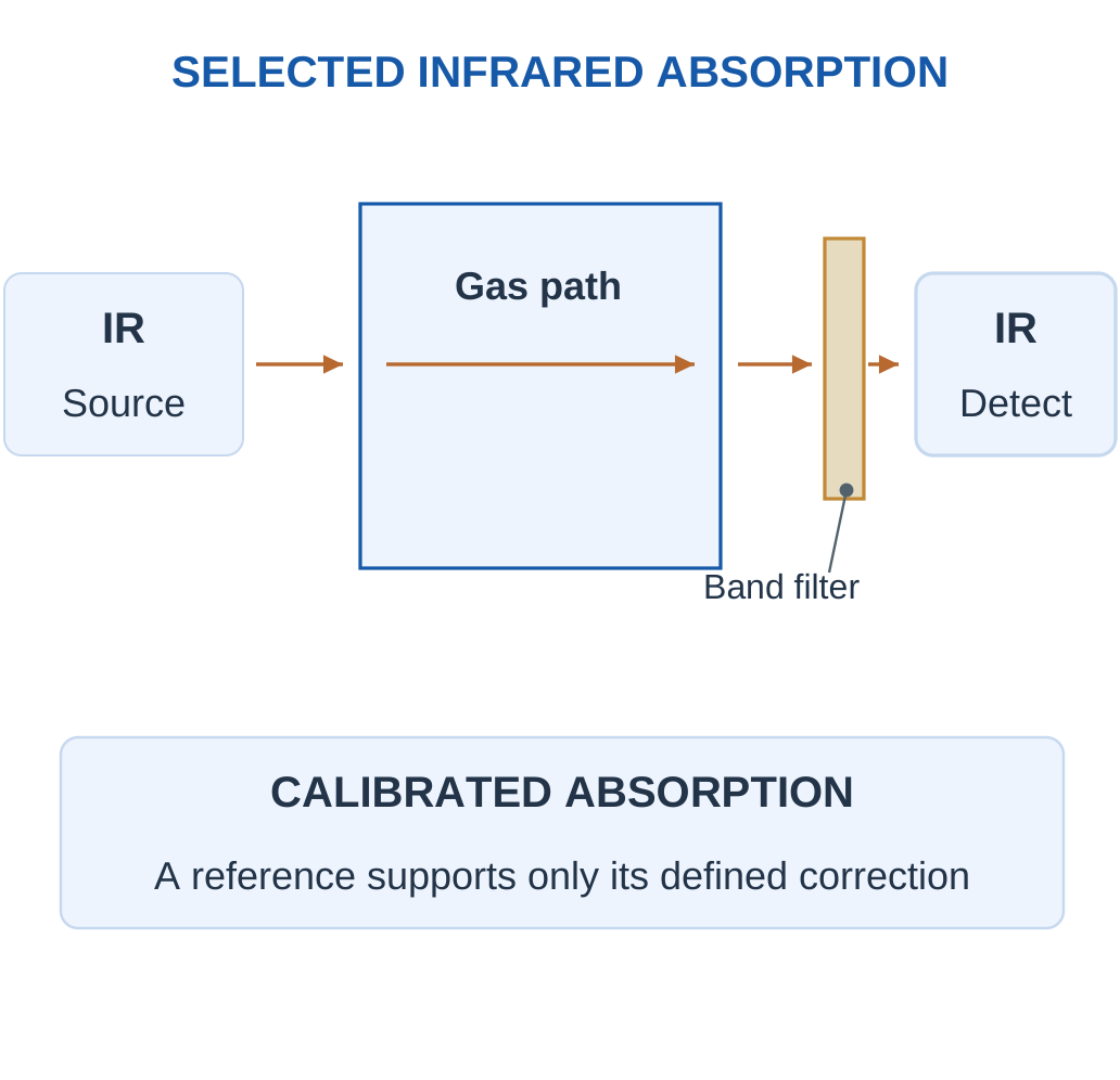
A non-dispersive infrared gas sensor uses absorption in selected infrared wavelength bands. A source illuminates the gas path, and filtered detection measures a target-sensitive band. Suitable reference channels or models can help account for source and other changes within their assumptions.
Key Idea: MEMS and Metal Oxide Can Both Describe One Sensor
A microfabricated hotplate can support a metal-oxide film. MEMS identifies the platform, while the oxide surface provides the stated chemical response. Treating them as mutually exclusive classes would misdescribe this combined device.

Chemical Selectivity Through Spectroscopy
A molecule must have a suitable absorption response in the chosen region. Carbon dioxide is a familiar infrared-absorbing example. The presence of a gas does not guarantee detection by every optical wavelength; homonuclear gases such as nitrogen do not show the same strong fundamental infrared response as common target bands used in basic NDIR.
Reference Correction
A ratio between target and reference channels may reduce certain common source variations if both channels are affected as assumed. Window contamination, wavelength-dependent loss, humidity and cross-absorbing species can still alter interpretation. A reference is evidence within a model, not a universal correction for all changes.
Path Length and Concentration
A longer suitable path can increase absorption sensitivity in the stated model but can also reduce transmitted light and alter dynamic/packaging requirements. Temperature and pressure affect gas state and optical response, so an arbitrary path-length change does not automatically improve every performance measure.
NDIR Versus a Complete Spectrometer
The selected filters/bands provide the intended non-dispersive measurement rather than a full spectrum separated by a scanning dispersive element. The key explanation is wavelength-selective gas absorption, not merely that a light turns on inside a sensor.
Arrow Rule
Show an optical beam through the gas region to the detector. Do not represent gas molecules as flowing through the electrical signal cable.
Worked Example 3.21: Apply a Defined Two-Channel Optical Ratio Model
Problem: A supplied optical gas exercise uses target/reference channels 60 and 100 units, with blank channels 100 and 100. Define corrected T = (target/reference)/(blank target/blank reference), then A = −log10 T and A = 0.02C for C in supplied concentration units. Find C.
Model / Approach: The ratio correction and calibration are explicitly defined. A second case can show common channel scaling. This simple model does not prove all wavelength-dependent contamination or cross-absorption is corrected.
Step 1: Sample target/reference = 0.6; blank ratio = 1.
Step 2: Corrected T = 0.6.
Step 3: Corrected absorbance A ≈ 0.221849.
Step 4: Inferred C = A/k ≈ 11.0924 supplied units. A ratio of one gives zero corrected absorbance in this stated convention.
Answer: Corrected T = 0.6; A ≈ 0.221849; C ≈ 11.0924 supplied units.
Check: A reference channel helps only for changes represented by its model.
Worked Example 3.22: Apply the Ratio Model to Common Channel Scaling
Problem: A supplied optical gas exercise uses target/reference channels 80 and 80 units, with blank channels 100 and 100. Define corrected T = (target/reference)/(blank target/blank reference), then A = −log10 T and A = 0.04C for C in supplied concentration units. Find C.
Model / Approach: The ratio correction and calibration are explicitly defined. This case shows common channel scaling. The simple model does not prove all wavelength-dependent contamination or cross-absorption is corrected.
Step 1: Sample target/reference = 1; blank ratio = 1.
Step 2: Corrected T = 1.
Step 3: Corrected absorbance A = 0.
Step 4: Inferred C = A/k = 0 supplied units. A ratio of one gives zero corrected absorbance in this stated convention.
Answer: Corrected T = 1; A = 0; C = 0 supplied units.
Check: A reference channel helps only for changes represented by its model.
17. MEMS-Based Gas Sensors and Micro-Hotplates
MEMS means micro-electromechanical systems. It describes a small-scale fabrication/platform approach, not one universal chemical-detection mechanism. A micromachined structure can support a heated metal-oxide film, an infrared emitter, a thermal-conductivity element or another appropriate transduction arrangement.


What to Notice
This is an illustrative view rather than a measured micrograph. MEMS describes the platform, while a film, thermal element or optical structure supplies its particular sensing mechanism. Packaging and interconnects link that small region to a usable instrument.

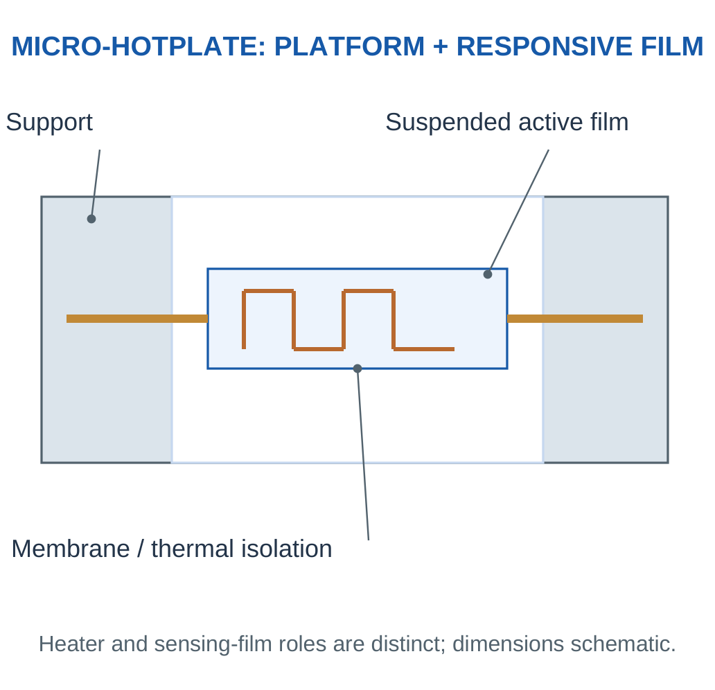
Micro-Hotplate Role
A small thermally isolated region can heat a sensing film with less required thermal mass than a large bulk structure. The relevant power, temperature response and mechanical/environmental durability still depend on its design. Miniaturisation does not automatically guarantee chemical selectivity or zero energy use.
Thermal Gas Sensing
A thermal-conductivity or calorimetric arrangement responds to heat transfer influenced by gas properties and conditions. That is distinct from a metal-oxide surface reaction even when both use heaters. Flow and gas composition can affect a thermal signal, so the stated purpose and calibration must be clear.
Mechanical Functionalisation
A responsive coating on a microstructure can change mass, stress or other properties, which a suitable transducer detects. The coating supplies the chemical interaction and the microstructure supplies a physical platform. A frequency or displacement shift is not automatically unique to one chemical species.
Compare Correctly
Metal oxide names a material/mechanism family, optical names a transduction approach, and MEMS names a platform. The categories can overlap; they should not be presented as completely exclusive boxes.
Worked Example 3.23: Separate Heater Active Power from Average Energy
Problem: A supplied micro-hotplate paper model uses heater power 30 mW for 1 s in each 10 s cycle and zero heater power otherwise. Find heater energy per cycle and average heater power.
Model / Approach: Only the defined heater electrical consumption is counted. Sensing electronics, warm-up kinetics and permissible temperature operation are not supplied; the cycle is an arithmetic input, not an operating recommendation.
Step 1: Active heater power is 0.03 W.
Step 2: Heater cycle energy is Pheat × active time = 0.03 J.
Step 3: Average heater power is cycle energy/cycle duration = 3 mW.
Step 4: The complete sensor could consume additional energy. Short duty time does not prove the chemistry reaches its required state or response fraction.
Answer: Cycle energy = 0.03 J; average heater power = 3 mW.
Check: MEMS can support reduced thermal mass, but its platform label alone does not establish a complete power budget or chemical response time.
18. Biosensor Architecture and Biological Recognition
A biosensor couples a biological recognition function to a measurable signal. Enzymes, antibody–antigen interactions and nucleic-acid recognition are examples. The biological part provides a selective chemical interaction, while the transducer may be electrochemical, optical or another physical type.
Key Idea: A Biological Sample Alone Does Not Define a Biosensor
An optical or electrical measurement of a biological sample can be useful without using a biological recognition element. A biosensor explanation should name the enzyme, immune interaction, nucleic-acid recognition or other biorecognition and connect it to the transducer.

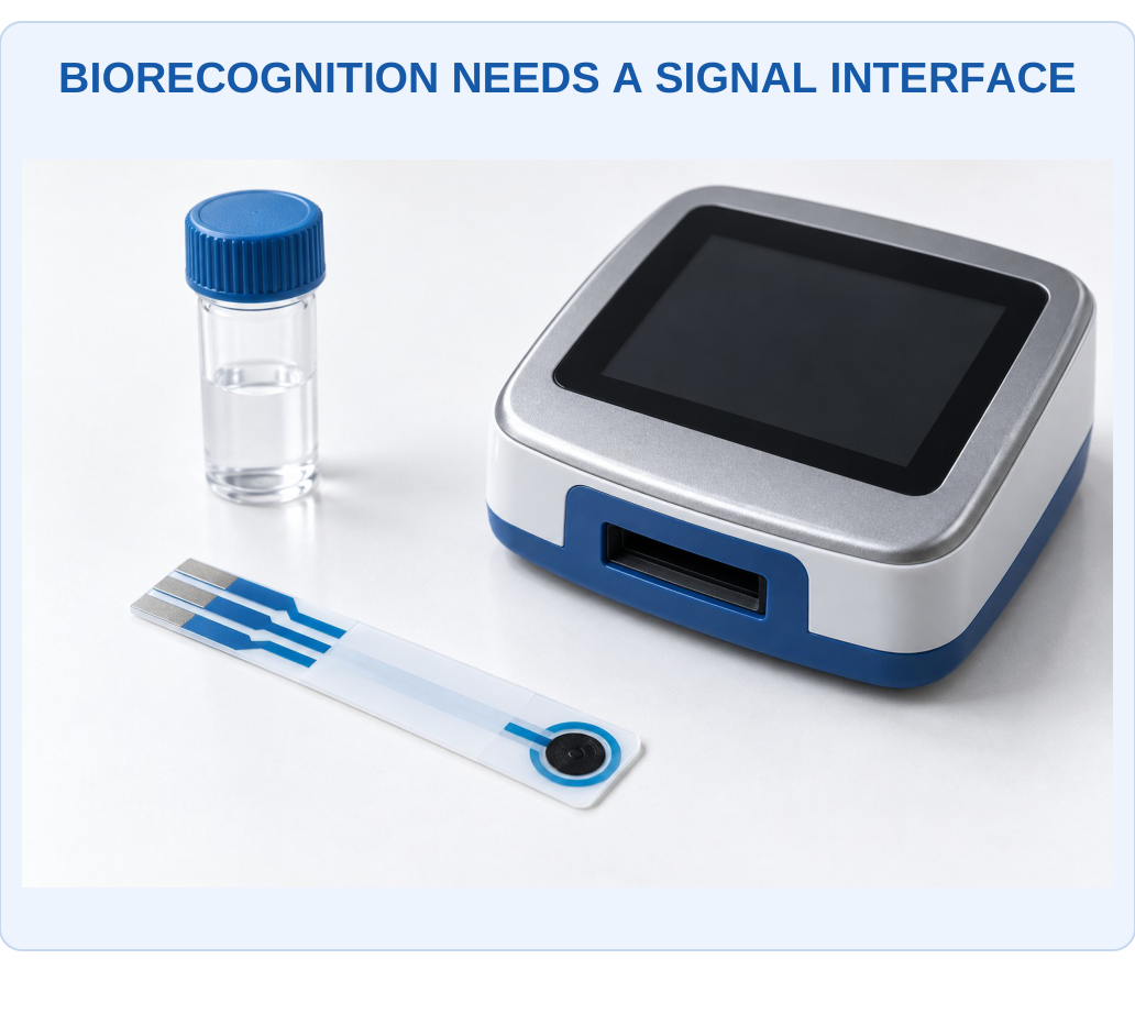
What to Notice
The appearance does not identify the biological recognition material or validate a diagnostic use. An enzyme, immune interaction or nucleic-acid layer must be connected to a defined transduction mechanism and calibration. The following diagrams explain that missing chemical chain.

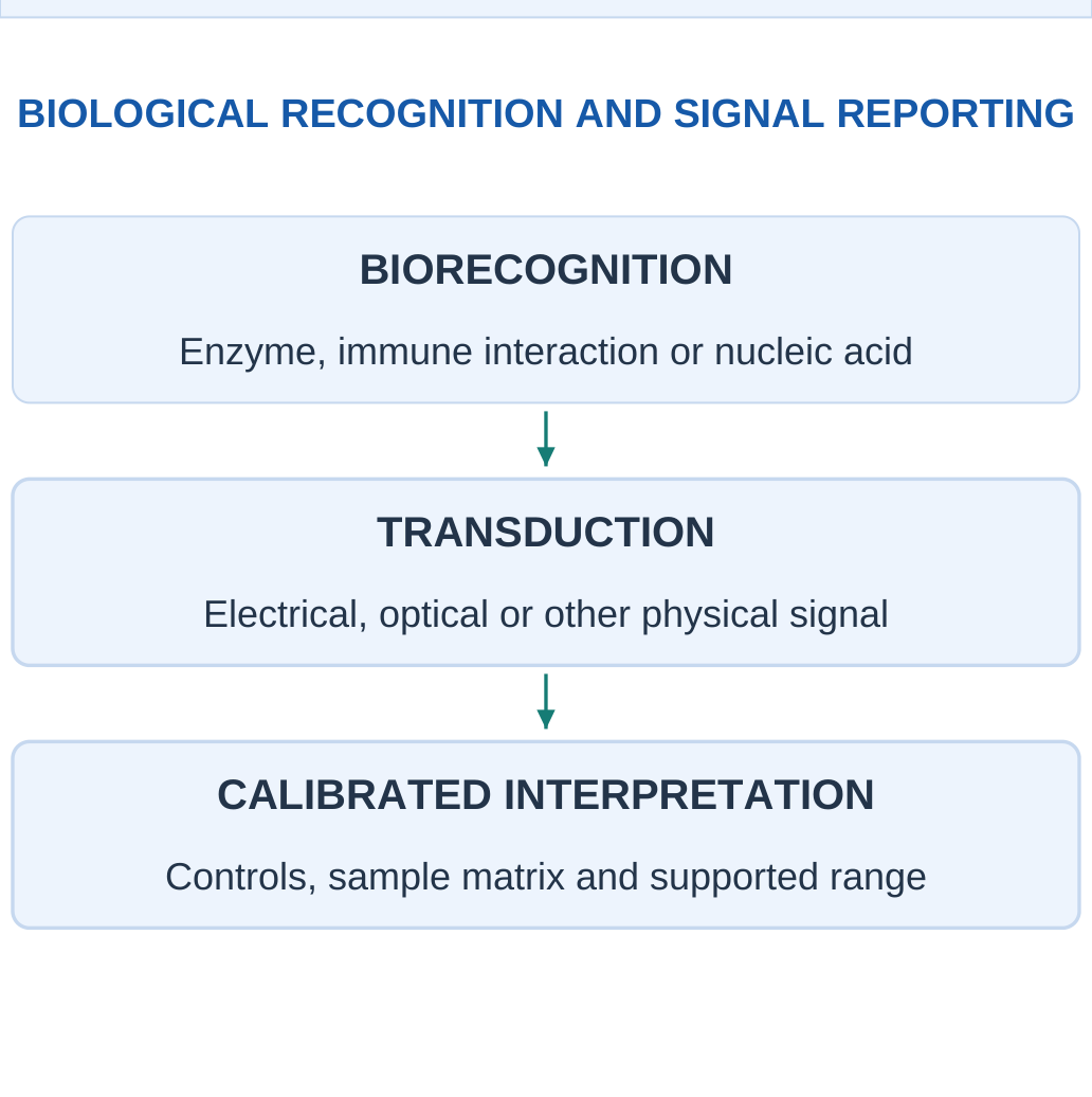
Immobilisation
An immobilised recognition layer is retained near the transducer so its interaction can be measured usefully. Attachment can affect activity, orientation, stability and access to the target. Simply adding more recognition material does not guarantee better response if diffusion or active-site accessibility becomes limiting.
Sample Matrix
Other sample components can cause nonspecific adsorption, inhibit a reaction or affect the transducer directly. A response in a simple standard does not automatically validate a complex real sample. Blanks, controls and appropriate calibration help distinguish target-related behaviour from background.
Reusable and Single-Use Designs
A reusable device needs appropriate recovery/regeneration while retaining useful recognition function. A single-use assay can instead preserve a captured signal for one measurement. The intended use affects how binding strength, stability and response time are evaluated.
Terminology Boundary
A sensor used on a biological sample is not automatically a biosensor if it has no biological recognition function. Conversely, a biosensor can be used for environmental or food analysis rather than only a medical application.
Answer Chain
Biorecognition event → chemical/physical change near the interface → transducer signal → calibrated interpretation.
Naming an enzyme or antibody alone does not explain how the information becomes measurable.
19. Enzyme Sensors: Glucose-Oxidase Example
An enzyme catalyses a reaction involving its suitable substrate. In a simple oxygen-dependent glucose-oxidase example:
Glucose + O2 → Gluconolactone + H2O2
This is followed by appropriate product chemistry in water. The enzyme is a catalyst rather than a reagent consumed once for every product molecule in the ideal cycle.


How the Reaction Becomes a Signal
A first-generation example can observe oxygen consumption or peroxide-related current. Other designs can use mediators or different electron-transfer arrangements. The chosen signal must be stated; “enzyme detects glucose” is incomplete without identifying the coupled observation.
Limiting Factors
Oxygen availability, substrate transport, enzyme activity, temperature and interfering electroactive species can affect response. If oxygen is limiting in the stated reaction model, increasing glucose alone cannot indefinitely increase reaction rate. A linear concentration relation therefore has a supported range.
Saturation Model
An optional supplied rate model is:
v = vmaxC/(Km + C)
It illustrates increasing response followed by saturation. Km is the concentration giving half vmax in that model. It is not automatically identical to a general sensor detection limit or the concentration range of every product.
Calibration and Use
A numerical glucose-sensor example here is an educational analytical model. Its concentration/current result is not a diagnosis, treatment instruction or a substitute for a validated clinical method. The general lesson is chemical coupling, interference and calibration.
Memory Cue
An enzyme provides catalytic recognition; the transducer measures a linked change. Catalysis does not remove the need for reactants, transport or appropriate operating conditions.
Worked Example 3.24: Evaluate a Supplied Saturating Enzyme-Rate Model
Problem: A supplied ideal enzyme example has vmax = 10 rate units, Km = 2 mM and substrate C = 1 mM. Use v = vmaxC/(Km + C). Find rate and fraction of vmax.
Model / Approach: The equation and parameter values are given for this educational reaction condition. They do not establish a universal glucose-sensor calibration, clinical interpretation or equality between Km and a detection limit.
Step 1: Denominator Km + C = 3 mM.
Step 2: Rate v = 10 × 1/3 ≈ 3.33333 supplied rate units.
Step 3: Fraction of vmax is approximately 0.333333, or 33.3333%.
Step 4: At C = Km the model would give half vmax. Increasing C indefinitely approaches vmax rather than increasing the response linearly without limit.
Answer: Rate ≈ 3.33333 units; approximately 33.3333% of vmax.
Check: Check whether the supplied concentration belongs to a linear low-concentration approximation or a saturating model before inverting a sensor signal.
20. Immunosensors and Antibody–Antigen Recognition
An immunosensor uses an immunological binding interaction coupled to a transducer. A surface-bound antibody can capture a suitable antigen, or another defined arrangement can be used. The binding partner, target and signal pathway must be identified explicitly.

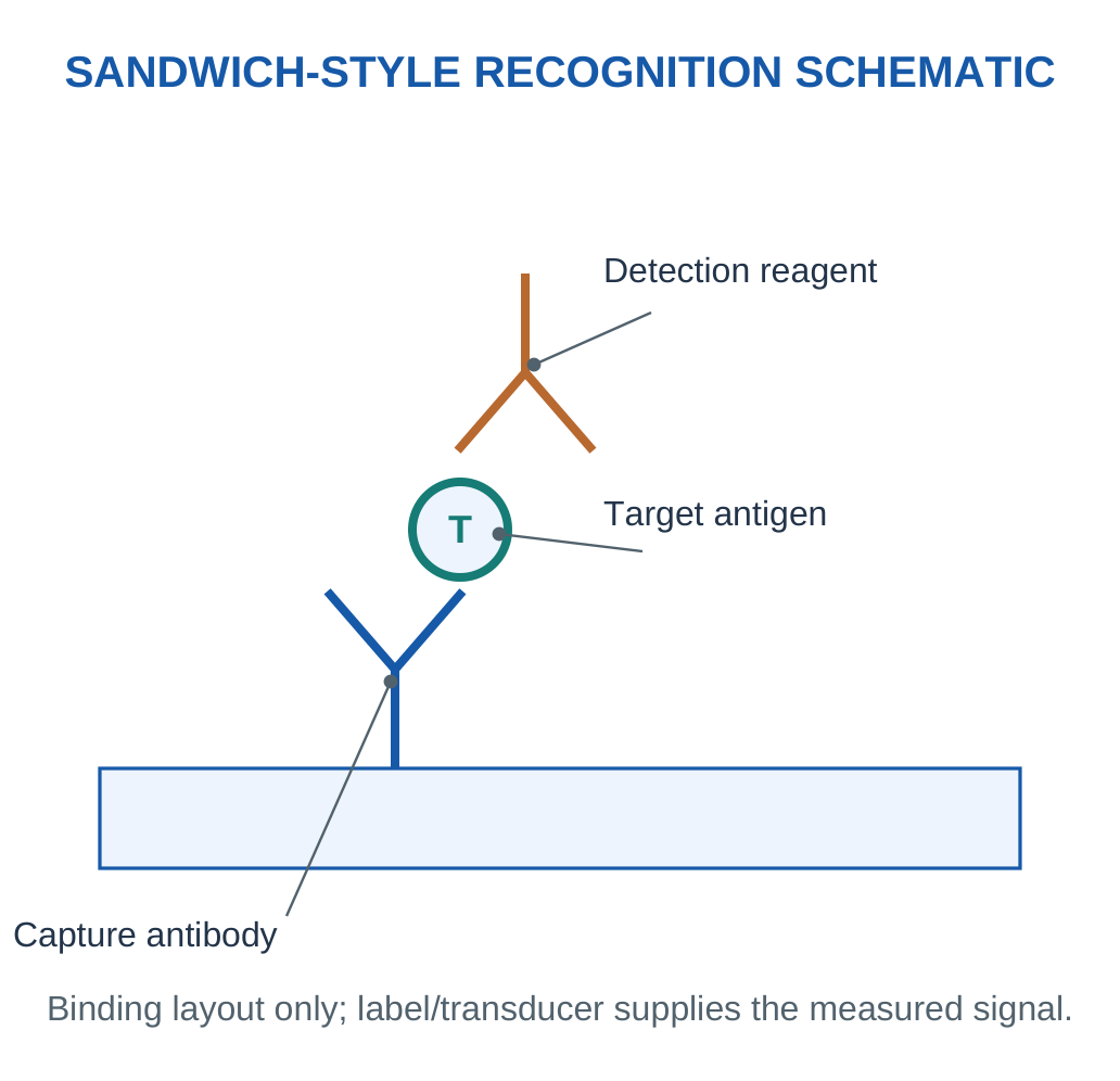
Direct and Labelled Approaches
A label-free measurement observes a physical change associated with binding, such as an electrical or optical interface response. A labelled approach uses an attached signal-generating species or reagent. Neither label-free nor labelled automatically means more accurate for every sample.
Sandwich and Competitive Formats
A sandwich format requires target recognition that supports the defined capture and detection arrangement. A competitive format instead uses competition to relate signal to target amount and may give a decreasing signal with increasing target. The sign of the response must follow the stated assay format.
Selectivity Is Conditional
Affinity and recognition can improve selectivity, but cross-reactivity and nonspecific binding remain possible. A background control addresses a particular non-target contribution; it does not establish that every other compound is absent or nonresponsive.
Saturation and Calibration
Finite binding sites can lead to nonlinear response. A supplied ideal occupancy model is:
θ = C/(Kd + C)
It may support conceptual calculations, but a complete analytical signal also depends on the transducer and assay conditions. Occupancy is a fraction, not concentration by itself.
Diagram Rule
Label capture antibody, target and detection reagent separately. The two arms of a drawn antibody must not be mistaken for two separate sensor wires.
Worked Example 3.25: Interpret an Ideal Binding Occupancy Separately from Signal
Problem: A supplied ideal binding model is θ = C/(Kd + C), with Kd = 2 nM, C = 2 nM and 100 equivalent site units. Find occupancy and expected occupied-site units.
Model / Approach: Use the stated equilibrium occupancy model only. The site units are an illustrative average count; optical/electrical signal, kinetics, cross-reactivity and real assay performance are not defined by occupancy alone.
Step 1: Denominator Kd + C = 4 nM.
Step 2: Occupancy θ = 2/4 = 0.5.
Step 3: Expected occupied-site units are θ × total = 50.
Step 4: Unoccupied units are 50. Occupied plus unoccupied recovers the supplied total, with 0 ≤ θ ≤ 1.
Answer: Occupancy = 50%; occupied-site units = 50.
Check: A fractional occupancy is not a concentration unit and is not automatically the measured signal without a defined transduction relation.
21. DNA Sensors and Complementary Hybridisation
DNA recognition can use a known single-stranded probe that binds a complementary target sequence under suitable conditions. Base pairing follows A with T and G with C in the basic DNA model, and the paired strands run antiparallel. The probe sequence and orientation therefore matter.


What to Notice
Different spots can carry defined probes in an appropriate assay. The visible array is a physical layout, not a sequence result. Complementary pairing, strand direction, reporting chemistry and evaluated controls still determine the information that can be obtained.


For probe 5′-ATGC-3′, a directly aligned complement is 3′-TACG-5′. If that complementary target is written in its own 5′→3′ direction, it is 5′-GCAT-3′. Reversing the writing direction is not the same as changing the base-pair rule.
How Hybridisation Produces Information
A label can provide an optical/electrochemical response, or binding can change an interface property measured by a suitable transducer. The recognition event is complementary association; the actual signal still needs a physical reporting mechanism and calibration.
Mismatches and Conditions
Temperature, ionic environment, sequence and nonspecific adsorption affect hybridisation. A single mismatch can influence binding, but a generic drawing cannot guarantee perfect discrimination under every condition. Controls and supported assay conditions determine what the result can justify.
What a DNA Sensor Is Not Automatically
Hybridisation does not inherently perform full genome sequencing or amplify the target. Amplification and sequencing are additional methods with their own functions. A positive response to a defined probe concerns that validated recognition task, not every possible sequence in the sample.
Sequence Habit
First draw both strand directions, then pair bases, then rewrite a reverse complement only if the requested direction changes. This avoids a common correct-bases/wrong-orientation error.
Worked Example 3.26: Write an Antiparallel Complement and Reverse Complement
Problem: A model probe is written 5′-ATGC-3′. Give the directly aligned complementary strand and then write that complementary target in its own 5′→3′ direction.
Model / Approach: Use the basic DNA pairing A–T and G–C with antiparallel strand directions. This is a sequence-orientation exercise, not a prediction of binding selectivity or a complete assay protocol.
Step 1: Pair bases position by position to obtain TACG.
Step 2: Because strands are antiparallel, the aligned complement is 3′-TACG-5′.
Step 3: Reverse the written order to express that target as 5′-GCAT-3′.
Step 4: The reverse complement has the same base-pair relationship with proper orientation. Complementing alone and labelling it 5′→3′ would give a different sequence.
Answer: Aligned complement = 3′-TACG-5′; target written in its own direction = 5′-GCAT-3′.
Check: Correct letters with wrong strand direction are not a correct hybridisation drawing.
22. Biosensor Controls, Recovery and Useful Signal
A valid interpretation separates target recognition from the background of the complete measurement. Useful checks can include a blank, a defined non-target control, a known positive sample or a spike/recovery comparison. Each answers a specific question rather than certifying every property at once.

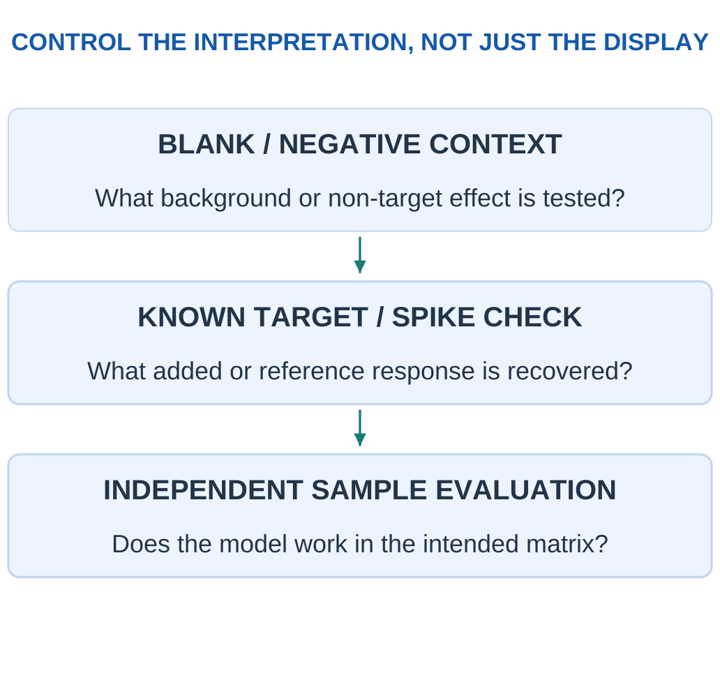
Spike Recovery
For a supplied additive-concentration model:
Recovery (%) = (Measured Spiked − Measured Original)/Added Amount × 100
Subtracting the original is essential; dividing the entire spiked result by the added amount would count target already present.
Matrix Effects
A complex sample can change recognition or signal conversion. A calibration in a simple buffer may not transfer unchanged. Dilution can reduce some effects but also lower the target signal; it is not a universal correction for every interfering process.
Detection Decisions
A supplied threshold rule can be evaluated with a defined set of labelled samples. Sensitivity in that classification context means a true-positive fraction, which differs from the analytical slope also called sensitivity. Specificity concerns the defined true-negative fraction. Keep the two meanings clearly labelled.
Evidence Limit
A small educational confusion matrix reports outcomes in its specified dataset. It is not proof of clinical performance, population predictive value or a medical recommendation. The broader validation task requires appropriate samples, conditions and uncertainty assessment.
Read the Denominator
Analytical sensitivity uses signal change/input change.
Classification sensitivity uses true positives/all actual positives.
They have different units and meanings even though they share a word.
Worked Example 3.27: Calculate Recovery of an Added Concentration
Problem: A supplied additive sample model measures original 5 mg/L and spiked 8.8 mg/L after addition equivalent to 4 mg/L on the same final basis. Calculate spike recovery.
Model / Approach: The addition and measurements are already expressed on the same specified volume/concentration basis. Use the increment, not the entire spiked value. No acceptance limit is invented.
Step 1: Measured increment is 8.8 − 5 = 3.8 mg/L.
Step 2: Recovery fraction is increment/added = 0.95.
Step 3: Recovery percentage is 95%.
Step 4: The result compares the added target increment under this model. It does not by itself establish that every endogenous target fraction or all other matrices are measured correctly.
Answer: Supplied spike recovery = 95%.
Check: Dividing the full spiked concentration by added concentration would include target already present and misstate recovery.
Worked Example 3.28: Keep Classification Sensitivity Distinct from Calibration Slope
Problem: A supplied labelled classroom dataset has true positives 18, false negatives 2, true negatives 27 and false positives 3. Calculate classification sensitivity, specificity and overall accuracy for this dataset.
Model / Approach: Use the given true class labels and binary decisions. These counts are educational data, not evidence of clinical performance, population predictive values or an appropriate medical decision threshold.
Step 1: Actual positives total 20; sensitivity TP/(TP + FN) = 90%.
Step 2: Actual negatives total 30; specificity TN/(TN + FP) = 90%.
Step 3: All cases total 50; correct cases 45, giving accuracy 90%.
Step 4: These are unitless fractions of labelled outcomes. Analytical sensitivity in mV per concentration unit is a different quantity.
Answer: Classification sensitivity = 90%; specificity = 90%; accuracy = 90%.
Check: State the denominator before calculating.
23. RFID Tags: Communication and Materials
Radio-frequency identification uses a reader and a tag to exchange identifying information. A passive tag obtains operating energy from the reader’s electromagnetic field through its supported coupling arrangement. Its antenna, integrated circuit and substrate form a functional material/electrical system.
Key Idea: Passive Does Not Mean Energy-Free
A passive tag receives the relevant operating energy from the reader through supported coupling. A failed read can therefore result from poor energy transfer or geometry as well as material damage. Unreadability alone cannot be labelled a unique chemical exposure.

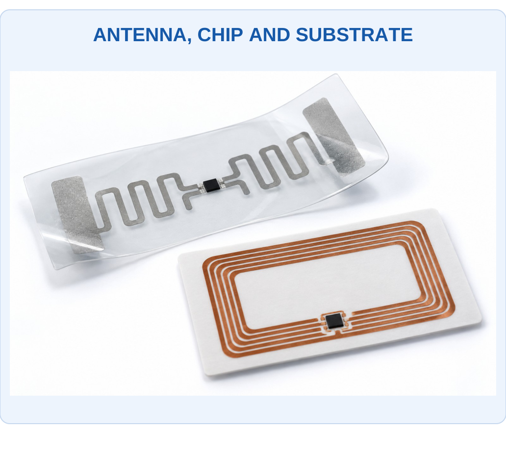
What to Notice
The tag first provides a communication and energy-coupling function. Chemical sensing requires a responsive material or sensor interface in addition to identification. Geometry, bending and surrounding materials can also change the RF response and need to be distinguished from target exposure.

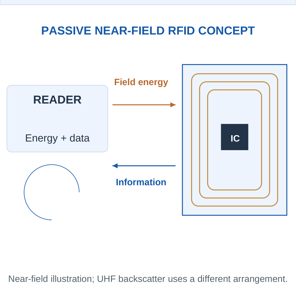
Different Frequency/Coupling Approaches
A near-field arrangement can use inductive coupling and load modulation. A suitable far-field UHF arrangement can use backscatter. These are not identical mechanisms, and no single coil drawing establishes every RFID system’s range or frequency behaviour.
Tag Material Chemistry
Conductive antenna materials can include metals or suitable conductive inks. Polymer/paper substrates and adhesives support the structure. Oxidation, bending, moisture and chemical exposure can change conductivity, adhesion or dielectric behaviour. A tag’s useful read response therefore depends on its complete construction and environment.
Passive Does Not Mean Unpowered
A passive tag has no independent battery in the stated passive concept, but it still needs energy for its electronic response. The reader supplies the relevant energy path. A tag that cannot be read may be out of range, poorly coupled, damaged or otherwise affected; unreadability is not uniquely a chemical alarm.
Distinguish the Functions
RFID identifies/communicates. A chemically responsive layer or connected sensor can add chemical information. An ordinary identification tag does not automatically measure gas concentration because its antenna is metallic.
Worked Example 3.29: Report a Defined RFID Read-Success Fraction
Problem: A supplied test records 92 successful reads in 100 defined attempts under one fixed geometry and environment. Calculate observed read-success and failure fractions, and state what chemical claim they do not establish.
Model / Approach: Each attempt has a defined binary outcome and the same counted basis. No statistical population model, chemical calibration or cause of failed reads is supplied.
Step 1: Read-success fraction is 92/100 = 0.92.
Step 2: Observed success percentage is 92%.
Step 3: Failed attempts are 8, giving 8%.
Step 4: Success and failure fractions sum to one. They describe communication outcomes in this test, not automatically target concentration or a unique exposure state.
Answer: Observed success = 92%; failure = 8%.
Check: Unsuccessful communication can have geometry, energy, damage or environmental causes.
24. Chemically Responsive RFID Sensing
A chemical RFID sensor couples a responsive material or sensing unit to a tag/readout. Analyte exposure may change resistance, capacitance, dielectric behaviour or another property that influences the electronic response. The reader interprets that change using an appropriate calibration and control of other influences.

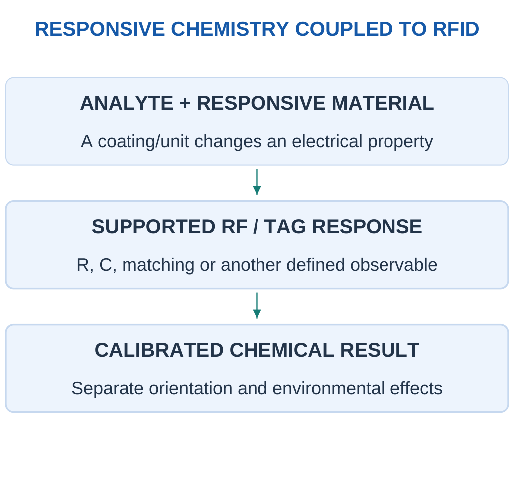
Material to Electrical Response
A conducting-polymer film may change resistance through chemical interaction. A humidity-responsive region may change dielectric properties. Other coatings can recognise different targets. These are examples of functional coupling, not a claim that every tag coating is selective or reusable.
Resonance Support Model
For a deliberately supplied ideal LC model:
f0 = 1/(2π√LC)
If L remains fixed and C increases, f0 decreases. The model is useful for a paper sensitivity calculation but does not represent all chip/antenna impedance, coupling, loss and reader-processing behaviour of a real RFID sensor.
Controls and Calibration
Read distance, orientation, surrounding materials and temperature can affect a tag response. A separate reference feature or baseline can help test particular confounders. A signal change cannot be assigned uniquely to target chemistry without evidence that other relevant influences are controlled or represented.
Applications and Limits
Suitable tags can support distributed monitoring of packaging, exposure or environmental conditions. The claimed measurand and evidence should be clear: identification, a threshold exposure indication and a quantitative concentration are different functions.
Answer Chain
Responsive chemistry → changed electrical property → changed supported RF measurement → calibrated chemical interpretation.
Do not skip directly from a printed antenna picture to a quantitative pollutant claim.
Worked Example 3.30: Use a Supplied Ideal LC Response to a Capacitance Change
Problem: A paper tag-support model has L = 1 µH and C = 100 pF. A supplied responsive effect multiplies C by 1.21 while L remains fixed. Use f0 = 1/(2π√LC). Find initial/final frequency and relative change.
Model / Approach: This is an ideal lossless lumped LC calculation. Real antenna/chip matching, coupling and the chemical selectivity of the responsive layer are outside the given model; these values are not a product configuration.
Step 1: Convert L = 1 × 10⁻⁶ H and C = 1 × 10⁻¹⁰ F.
Step 2: Initial f0 ≈ 15.9155 MHz.
Step 3: Changed frequency is approximately 14.4686 MHz, with ratio f1/f0 = 1/√1.21 ≈ 0.909091.
Step 4: Relative frequency change is approximately −9.09091%. This sign follows the supplied capacitance change rather than every possible tag exposure.
Answer: Initial frequency ≈ 15.9155 MHz; final frequency ≈ 14.4686 MHz; change ≈ −9.09091%.
Check: The ideal RF calculation does not itself prove which chemical caused C to change.
25. Environmental Chemical Detection in Water
Environmental water measurements can target pH, specific dissolved species, oxygen-related quantities or other chemical indicators. Different sensors observe different properties. A pH electrode cannot automatically measure total dissolved salts, and a conductivity value cannot uniquely identify one dissolved metal.

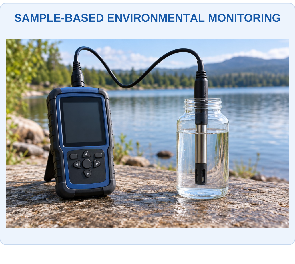
What to Notice
A field setting does not make one probe a universal water analyser. Identify the actual measurand, sample fraction, temperature and calibration. Preparation factors and time/location records connect the result to the environmental question.
Key Idea: A Prepared Dissolved Fraction Is Not Automatically Total Content
Filtering or extraction can change which target fraction reaches a sensor. A concentration in the final solution therefore needs its stated preparation basis. A dilution correction alone cannot recover an unmeasured particle fraction or an unknown extraction loss.
Key Idea: Missing Time Is Not Zero Concentration
A mean based on three represented hours does not automatically describe a four-hour interval when one hour is missing. Assigning the missing hour zero lowers the result without evidence. Report coverage and use the denominator defined by the actual represented data.

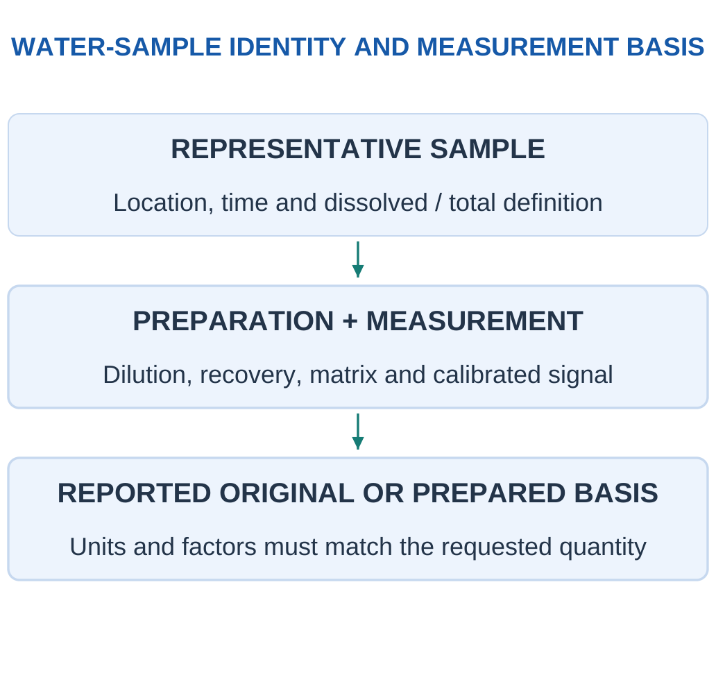
Sampling and Preparation
Location, time, container, filtration and dilution can change what the measurement represents. Dissolved and particle-associated material may be different fractions. A sensor result for a prepared sample must not be described as total original content without the appropriate preparation and recovery model.
Calibration in Context
Temperature, ionic strength, matrix composition and interfering species affect different methods. A matched standard or independent check supports the intended relation. A result within a display range is not the same as a validated result within the chemical working range.
Trace-Level Measurements
At low target levels, contamination, blank and adsorption losses can matter strongly. A small electrical output is not automatically a true low concentration; it may also indicate an unsuitable sensor state or preparation loss. The experiment/model must provide the basis for interpretation.
Reporting
State concentration units and whether the basis is the measured solution or original sample. Include any supplied dilution or recovery correction once.
Compare a reference or threshold only when its quantity, averaging definition and applicable context match; these notes do not invent environmental legal limits.
Selection Example
Choose an ion-responsive method for a stated ion-activity task, an appropriate target-specific reaction/optical method for another analyte, and verify matrix/interference behaviour rather than treating one generic probe as a universal water-quality analyser.
Worked Example 3.31: Preserve Water-Sample Mass, Volume and Preparation Basis
Problem: A supplied prepared-water model assigns dissolved target mass 2 mg in final volume 500 mL. Original concentration is defined as 1 times prepared concentration, with no loss/reaction. Find both concentration bases.
Model / Approach: Use mg/L with volume converted to litres. The stated mass belongs to the prepared dissolved fraction; no particle-associated or unextracted target is silently added.
Step 1: Prepared volume is 500/1000 = 0.5 L.
Step 2: Prepared concentration is mass/volume = 4 mg/L.
Step 3: Original-basis concentration is D × prepared = 4 mg/L.
Step 4: Multiplying prepared concentration by prepared volume recovers 2 mg. The original correction is separate from this prepared-sample mass check.
Answer: Prepared = 4 mg/L; original = 4 mg/L.
Check: A dissolved-fraction result is not automatically total original content.
26. Environmental Air Monitoring and Data Quality
Air monitoring combines sensor chemistry with sample transport, location and data interpretation. A measurement near a source may differ from a background location because the air is not perfectly uniform. Inlet access, nearby surfaces, humidity and temperature can affect useful readings.

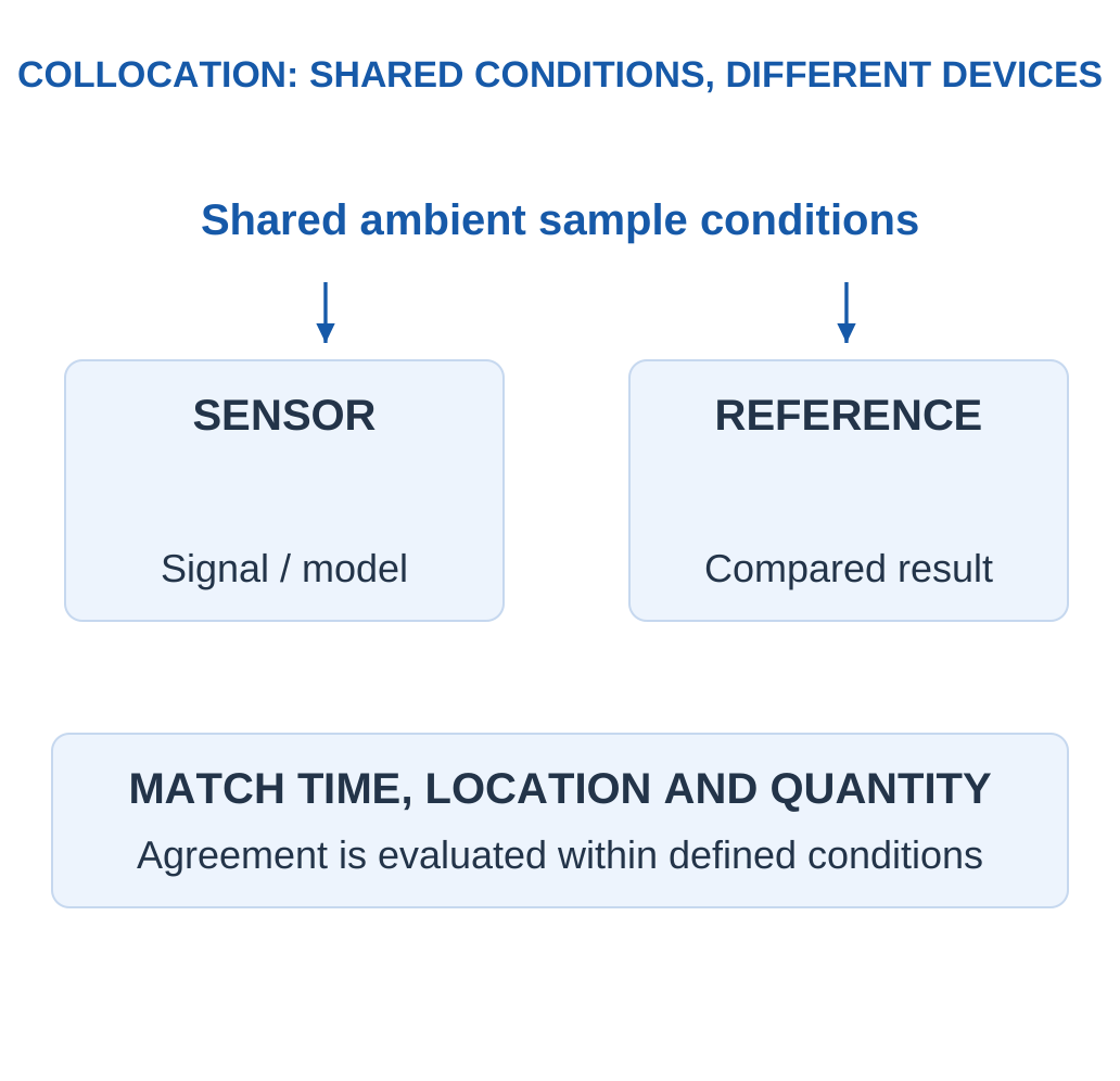
Collocation and Correction
Collocation operates a sensor and reference sufficiently together in time/location to evaluate comparable conditions. A supplied correction equation may reduce observed bias in the evaluated range. That mathematical correction is not proof that the underlying material has become perfectly selective or stable.
Time Averaging
A time-weighted average is:
ΣCiti/Σti
This applies when readings represent defined intervals. Missing intervals should not silently be assigned zero. A brief peak, a daily mean and a concentration-time integral answer different questions and need their own stated units/coverage.
Environmental Influences
Humidity may alter surface adsorption or optical conditions; temperature may change reaction or material transport. Cross-sensitive gases can add or subtract response. A model should include relevant influences or restrict its claimed conditions accordingly.
Interpretation Boundary
A low-cost sensor output can be useful evidence for a defined task, but a plotted number alone does not establish regulatory equivalence or a health conclusion. Use appropriate reference, validation and matching definitions for the actual decision.
Quality Habit
Record time, location, units, missing data and conditions along with the signal. A coloured map with many decimal places cannot repair poor sample representation or unverified chemical response.
Worked Example 3.32: Calculate a Time-Weighted Concentration Average
Problem: Supplied interval concentrations are [10, 30, 20] ppb with matching represented durations [1, 2, 1] h. Find the concentration-time sum and weighted average over these complete intervals.
Model / Approach: Each concentration represents its entire stated interval; no interval is missing. The result is an arithmetic environmental model and supplies no legal or health interpretation.
Step 1: Total represented time is 4 h.
Step 2: Sum of concentration × time is 90 ppb h.
Step 3: Time-weighted mean is sum/time = 22.5 ppb.
Step 4: The simple unweighted mean need not match when durations differ. Multiplying the weighted mean by total time recovers the concentration-time sum.
Answer: Integral = 90 ppb h; weighted mean = 22.5 ppb.
Check: A ppb h integral and a ppb mean have different units.
Worked Example 3.33: Apply a Supplied Collocation Correction Once
Problem: A supplied evaluated air-sensor correction is Ccorrected = 1.2Craw − 2, with both concentrations in ppb. Raw value is 20 ppb within the stated evaluation range. Find corrected value and change from raw.
Model / Approach: Use only the given affine correction at its supported conditions. This mathematical step does not establish universal environmental validity, chemical selectivity or regulatory equivalence.
Step 1: Multiplied raw term is 1.2 × 20 = 24 ppb.
Step 2: Add the supplied intercept to obtain 22 ppb.
Step 3: Change corrected − raw is 2 ppb.
Step 4: Inverting the same relation gives (corrected − b)/a = 20 ppb. Another unprovided offset must not be subtracted a second time.
Answer: Corrected concentration = 22 ppb; change = 2 ppb.
Check: Correction coefficients belong to an evaluated domain.
27. Flow, Residence Time and Sensor Dynamics
Sample transport creates a physical timing stage before or alongside the sensing reaction. For a supplied volume V and volumetric flow Q under matching conditions:
Nominal Residence Time = V/Q
This volume/flow ratio does not automatically equal the complete sensor’s t90.


Plug-Flow and Mixed-Volume Models
A simple ideal plug-flow delay moves a change after a stated travel time without mixing. A perfectly mixed volume instead approaches a new concentration exponentially when flow and volume are constant:
Fraction of New Input Reached = 1 − exp(−Qt/V)
Real arrangements can depart from either ideal.
Response Stages Combine
A transport delay plus a first-order sensor response gives a later reported threshold than either alone. Multiple dynamic stages are not always combined by simply adding their t90 values; use the model actually supplied. A problem may explicitly provide a fixed delay and one exponential stage for a manageable calculation.
Flow Reference
Gas flow specified at standard conditions and local volume at another state need a consistent conversion before V/Q is meaningful. Likewise, liquid and gas units or minutes and seconds must not be mixed silently.
Adsorption and Carryover
Tubing or chamber surfaces can retain species and release them later. This can distort both arrival and recovery beyond a pure volume/flow model. A delayed tail is not automatically an electronic fault or a new chemical source.
Dynamic Check
First identify whether the question supplies a delay, a mixed-volume flush, a sensor time constant or a complete measured response. Their names and units do not make them interchangeable.
Worked Example 3.34: Distinguish Nominal Residence Time from a Mixed-Volume Flush
Problem: A supplied perfectly mixed volume is 100 mL with constant matching flow 50 mL/min. New-input fraction is 1 − exp(−Qt/V). Find nominal residence time and time to 90% new-input fraction.
Model / Approach: Use the given well-mixed model, not a plug-flow delay. Volume and flow refer to the same state and phase; no adsorption, dead volume or separate sensor kinetics is included.
Step 1: Nominal residence time V/Q = 2 min.
Step 2: For fraction f, time is −(V/Q)ln(1 − f).
Step 3: Required time is approximately 4.60517 min = 276.31 s.
Step 4: At one residence time the model reaches about 63.2%, not 100%. A separate chemical sensor stage could add further dynamics.
Answer: Residence time = 2 min; requested fraction time ≈ 4.60517 min.
Check: V/Q and t90 have different definitions.
28. Electronic Nose: Arrays and Chemical Patterns
An electronic nose combines a sensor array with pattern-based data interpretation. Array elements may each be cross-sensitive, but their combined response pattern can distinguish classes represented by suitable training/validation data. It does not need one perfectly exclusive sensor for every possible molecule.

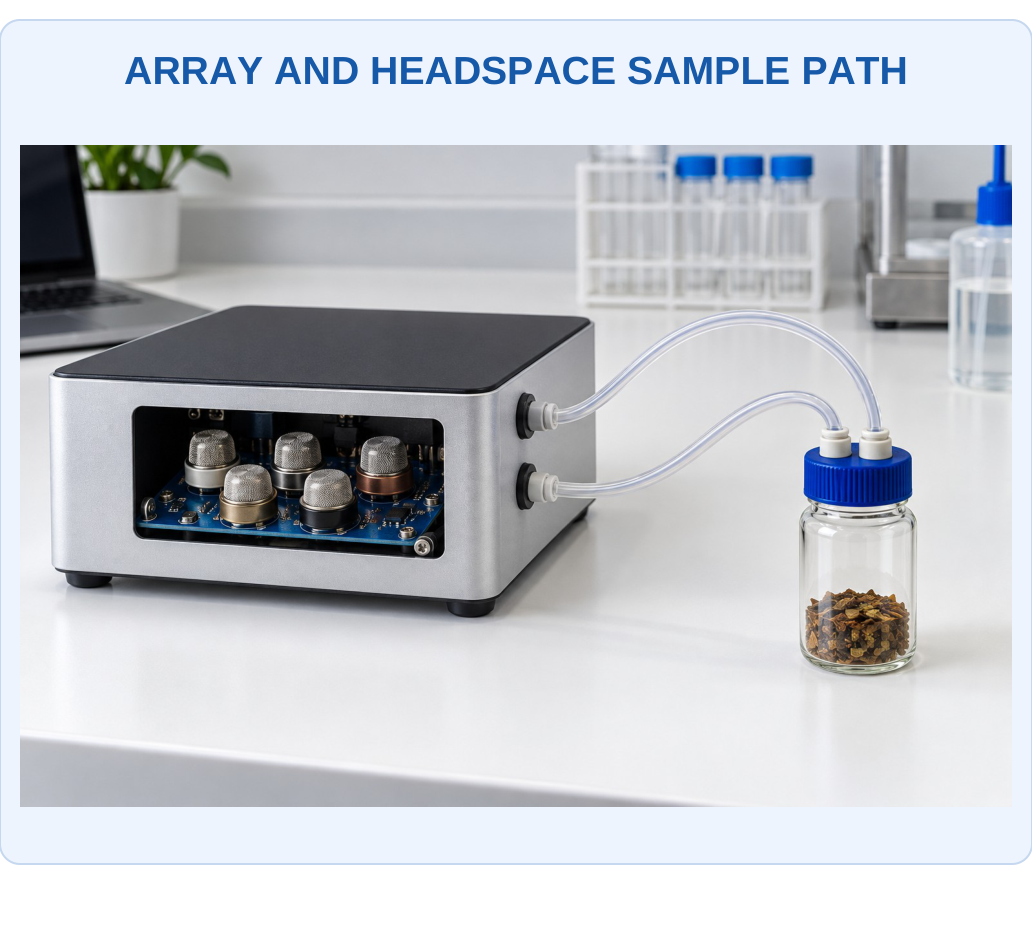
What to Notice
The collection of responses becomes a feature pattern under defined timing and environmental conditions. An array can support a validated class task, but its physical appearance cannot identify every molecule or prove that an unfamiliar mixture belongs to a known class.

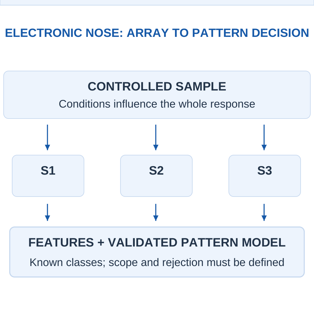
The Response Vector
If three sensors produce features r1, r2 and r3, one sample is represented by the vector [r1, r2, r3]. A normalised feature can use a stated baseline, such as:
(R − R0)/R0
The definition must be consistent across training and later samples.
Pattern Is Not Full Composition
A class label such as a defined packaging-headspace class is not automatically a list of all molecules or an exact target concentration. Classification and quantitative regression require different models and evidence. A mixture outside the known examples may resemble a trained class without truly belonging to it.
Sampling Consistency
Flow, humidity, temperature, exposure duration and recovery affect the pattern. A classifier can inadvertently learn these conditions rather than target chemistry if the dataset is poorly designed. Representative, separated validation is therefore part of the chemical-sensing system.
Uses
Appropriately validated arrays can support odour-related research, process monitoring and defined food/environmental comparisons. A generic e-nose illustration is not a universal diagnostic instrument or an assurance that every unknown gas is identified.
Analogy with Limits
The name nose refers to distributed pattern recognition. It does not mean the device literally reproduces human smell chemistry or can identify every possible odour without a supported dataset.
Worked Example 3.35: Build a Consistently Defined Array Feature Vector
Problem: A three-channel array has supplied baseline resistances [100, 80, 50] kΩ and exposed resistances [80, 88, 60] kΩ in the same order. Define each feature as (R − R0)/R0. Calculate the feature vector.
Model / Approach: Use the supplied baseline for each own channel. Resistances share units so the features are dimensionless; no class labels or target-specific concentration calibration are provided.
Step 1: Channel 1: (80 − 100)/100 = −0.2.
Step 2: Channel 2 gives 0.1; channel 3 gives 0.2.
Step 3: The vector is [−0.2, 0.1, 0.2].
Step 4: Positive/negative entries report relative resistance changes under this definition. The vector needs an evaluated pattern model before it can be assigned a chemical class.
Answer: Normalised vector = [−0.2, 0.1, 0.2].
Check: Changing the ratio definition or using one shared baseline for unequal channels changes the feature space and invalidates an unmodified stored classifier.
29. E-Nose Features, Classification and Validation
Array features can include a steady response, maximum change, slope, response time or recovery behaviour. Feature processing must use a consistent baseline and scale. Changing a feature definition after training changes what a stored reference pattern means.

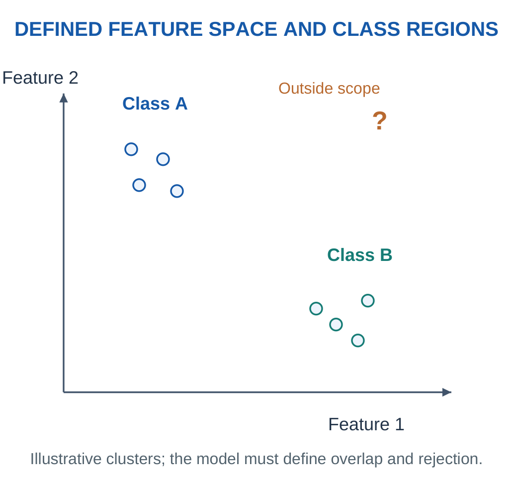
A Simple Distance Example
A supplied nearest-centroid model can compare squared distance:
d² = Σ(xi − μi)²
This is calculated for each stated class centre. The smaller distance selects a class only under the exercise’s decision rule. Different feature scales can dominate the distance unless the supplied preprocessing addresses them.
Training Versus Testing
Training data fit the model. Independent test data evaluate it. Closely repeated readings from the same exposure can share drift or sample history, so splitting those readings without respecting their dependence can exaggerate generalisation. A supported evaluation separates the relevant sample/session groups.
Confusion Counts
A labelled test set permits correct/incorrect fractions and class-specific errors. The denominator should match the requested quantity. Overall accuracy can hide unequal class performance, especially if one class dominates the dataset.
Rejecting Unsupported Inputs
A model can include a supplied distance or confidence criterion to reject a pattern too far from all known classes. That rule is not a proof of safety or a universal unknown-chemical detector, but it avoids pretending that every sample must fit one trained label.
Interpretation
Report the chosen model decision and its scope. A numerical distance is similarity in the specified feature space, not a chemical reaction mechanism or a validated concentration by itself.
Worked Example 3.36: Use a Stated Nearest-Centroid Rule with Rejection
Problem: A two-feature model has sample (0.2, 0.8), centre A (0.1, 0.9), centre B (0.8, 0.2). Use squared Euclidean distance. Select the nearer centre only when its squared distance is at most 0.1; otherwise reject. Find the model decision.
Model / Approach: Feature scaling and class centres are already supplied. The threshold is an educational rule, not a universal unknown-gas or safety criterion. Squared distance must be compared with the specified squared-distance threshold.
Step 1: Squared distance to A is 0.02.
Step 2: Squared distance to B is 0.72.
Step 3: The nearer centre is A with squared distance 0.02.
Step 4: Compare 0.02 with 0.1: decision is A. A forced label would ignore the stated rejection condition.
Answer: Model decision: A.
Check: Similarity in a defined feature space does not identify every molecule or establish a target concentration.
Worked Example 3.37: Reject a Pattern Outside the Supplied Distance Rule
Problem: A two-feature model has sample (1.5, 1.5), centre A (0.1, 0.9), centre B (0.8, 0.2). Use squared Euclidean distance. Select the nearer centre only when its squared distance is at most 0.2; otherwise reject. Find the model decision.
Model / Approach: Feature scaling and class centres are already supplied. The threshold is an educational rule, not a universal unknown-gas or safety criterion. Squared distance must be compared with the specified squared-distance threshold.
Step 1: Squared distance to A is 2.32.
Step 2: Squared distance to B is 2.18.
Step 3: The nearer centre is B with squared distance 2.18.
Step 4: Compare 2.18 with 0.2: decision is reject as outside the supplied distance rule. A forced label would ignore the stated rejection condition.
Answer: Model decision: reject as outside the supplied distance rule.
Check: Similarity in a defined feature space does not identify every molecule or establish a target concentration.
30. Drift, Fouling and Responsible Sensor Deployment
Chemical surfaces and biological recognition layers can change with time, exposure and storage. Fouling can obstruct access, poisoning can alter active sites, and environmental history can shift baseline or sensitivity. Drift is therefore part of the sensing chemistry as well as a data-processing problem.

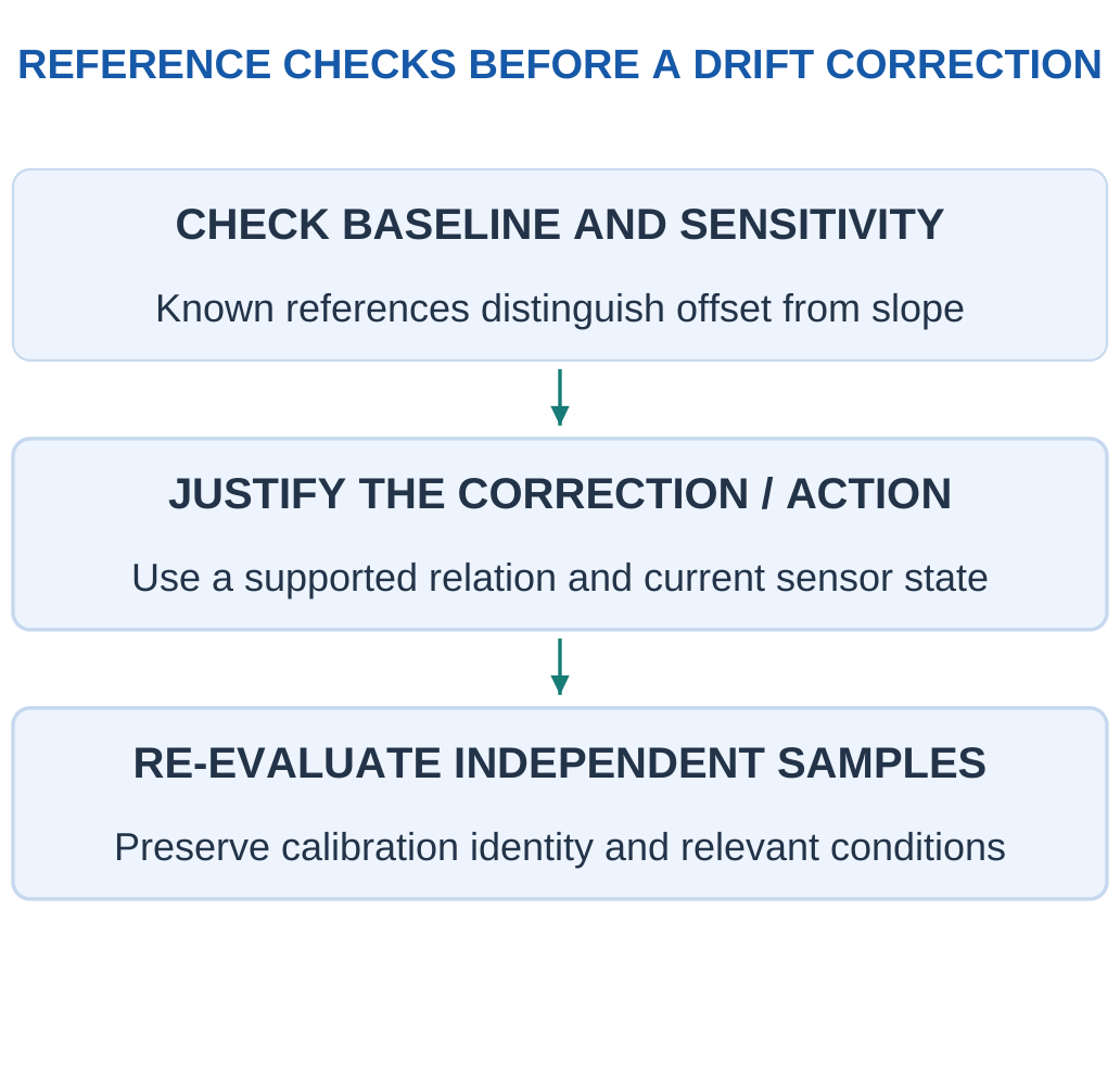
Offset and Slope Changes
If y = b + mC changes only by an additive offset, subtracting the known offset can restore the supplied model. If m changes, a zero correction alone leaves a concentration-dependent error. Two or more appropriate reference conditions can reveal this distinction in a simple model.
Array Drift
An e-nose can produce a different pattern for the same sample after material/environmental change. Correcting each channel or updating a model may help only when the assumed drift relation is valid. Relabelling new unknowns as though they were known references can contaminate a calibration.
Data and Maintenance
A record should preserve calibration identity, time, environmental conditions and changes in the measurement system. Replacing a sensing element can alter baseline and sensitivity even if the digital interface remains the same. An unchanged file format does not guarantee unchanged chemical performance.
Fit for Purpose
Select the sensor, sample arrangement and verification for the intended concentration, mixture, environment and decision. Critical uses require the relevant validated complete system. A classroom formula or an attractive display is not sufficient evidence by itself.
Final Field Question
Does the current sample and sensor state still belong to the conditions under which this calibration and decision rule were evaluated? If the evidence is missing, report that limit rather than inventing confidence.
Worked Example 3.38: Distinguish Additive Drift from Changed Sensitivity
Problem: Original calibration is y = 5 + 2C. A supplied later state is y = 8 + 2C. For true reference C = 10 mg/L, find later y, the old-calibration estimate and the estimate after correcting only the known intercept change.
Model / Approach: The later model and reference input are explicitly supplied for diagnosis. The correction removes b1 − b0 but retains the old slope; this tests what a zero-only correction can and cannot repair.
Step 1: Later signal is b1 + m1C = 28 signal units.
Step 2: Old inverse gives (y − b0)/m0 = 11.5 mg/L.
Step 3: After removing only intercept change, estimate is 10 mg/L.
Step 4: It recovers the reference because only the offset changed.
Answer: Later y = 28; old estimate = 11.5 mg/L; offset-only estimate = 10 mg/L.
Check: A baseline correction is not a universal sensitivity correction.
Worked Example 3.39: Examine a Changed Slope
Problem: Original calibration is y = 5 + 2C. A supplied later state is y = 5 + 1.8C. For true reference C = 10 mg/L, find later y, the old-calibration estimate and the estimate after correcting only the known intercept change.
Model / Approach: The later model and reference input are explicitly supplied for diagnosis. The correction removes b1 − b0 but retains the old slope; this tests what a zero-only correction can and cannot repair.
Step 1: Later signal is b1 + m1C = 23 signal units.
Step 2: Old inverse gives (y − b0)/m0 = 9 mg/L.
Step 3: After removing only intercept change, estimate is 9 mg/L.
Step 4: It does not recover the reference because the slope differs from the old model.
Answer: Later y = 23; old estimate = 9 mg/L; offset-only estimate = 9 mg/L.
Check: A baseline correction is not a universal sensitivity correction.
31. Formula Guide and Comparison Checkpoints
Calibration and Signal Quality
y = b + mC
C = (y − b)/m
Two-point slope:
m = (y2 − y1)/(C2 − C1)
Apply a supplied dilution factor to the correctly interpreted diluted result.
Signed Error = Measured − Reference
Percent error uses the stated reference denominator.
Sample standard deviation:
s = √[Σ(xi − xmean)²/(N − 1)]
This applies when that sample convention is specified.
A supplied simple blank-noise concentration estimate is:
3σblank/|m|
It is conditional on the stated noise/linearity convention, not a universal validation claim.
Electrochemistry
Amperometry controls potential and measures current.
Assigned reaction current:
I = zFr
Here r is in mol/s. Include a supplied assigned collection/current efficiency once.
A linear current model:
I = I0 + kC
needs its stated baseline and units.
Potentiometric ideal cation support:
E = E0 + (RT/zF)ln a
At the supplied 298 K base-10 convention:
E in mV = E0 + (59.16/z)log10 a
A given pH calibration may use:
E = E0 − S pH
pH = −log10 aH+
Concentration substitution requires the given approximation.
Gas and Optical Support
For the defined mole-fraction gas basis:
ppm = Fraction × 10⁶
ppb = Fraction × 10⁹
At a supplied ideal molar volume Vm in L/mol:
mg/m³ = ppm × Molar Mass in g/mol / Vm
Preserve the stated temperature/pressure.
T = I/I0
Percent Transmittance = 100T
A = −log10 T
Beer–Lambert supplied model:
A = εlc
A divider measured across RL uses:
Vout = VsRL/(Rs + RL)
Use the defined sensor-response ratio rather than inventing its sign.
Biology, Tags and Dynamics
Ideal enzyme rate when supplied:
v = vmaxC/(Km + C)
Ideal binding occupancy when supplied:
θ = C/(Kd + C)
Recovery (%) = (Spiked Measured − Original Measured)/Added Amount × 100
Probe/target directions are antiparallel; complement bases before rewriting a reverse complement.
Ideal LC support:
f0 = 1/(2π√LC)
Nominal residence time:
V/Q
First-order fraction reached:
1 − exp(−t/τ)
Therefore:
t90 = τ ln 10
Time-weighted mean:
ΣCiti/Σti
Use represented intervals.
Nearest-centroid squared distance:
Σ(xi − μi)²
This applies in the defined feature space.
Key Idea: Confirm a Concentration Through Back-Substitution
For y = b + mC, substitute the recovered prepared concentration into the same equation before applying dilution. This checks arithmetic and signal units. Then preserve the original-sample factor separately so that a correct signal inversion is not spoiled by a preparation error.
Comparison Checkpoints
| Do Not Confuse | Distinction |
|---|---|
| Slope sensitivity / classification sensitivity | Signal units per input / true-positive fraction |
| Resolution / accuracy | Represented step / agreement with relevant reference |
| MEMS / metal oxide | Platform / material-response family |
| RFID identification / chemical sensing | Communication / responsive measurand function |
| ppm / mg/m³ | Fraction basis / mass-volume basis |
| Sampling interval / t90 | Digital timing / physical response threshold |
Five Checks
Name the measurand, define the chemical mechanism, choose the correct signal model, convert units and explain the supported range. Correct arithmetic cannot create selectivity that the measurement has not established.
32. Short Questions with Complete Answers
1. What Is a Chemical Sensor?
It translates chemical information about a defined analyte or related quantity into a measurable signal through an appropriate interaction and transducer. Useful interpretation also needs calibration, sample context and operating conditions.
2. Is Sensitivity the Same as Selectivity?
No. Analytical sensitivity is the change of signal per change in input. Selectivity concerns the response relative to other influences. A steep response to several gases can be sensitive without uniquely identifying one gas.
3. Can a Sensor Be Repeatable but Biased?
Yes. Repeated readings can cluster around an average that differs from a supplied reference. Small spread and agreement with the reference are different measurement properties.
4. Why Does a Blank Matter?
It represents relevant background under its defined procedure/matrix. A blank helps interpret target-related signal, but it must not be subtracted again if the same baseline is already handled by the calibration intercept.
5. What Does an Amperometric Sensor Measure?
It measures current at a controlled electrode potential. The current can be related to target reaction/transport under the supplied calibration. Competing electroactive species or fouling can also affect it.
6. Why Separate Reference and Counter Electrodes?
The reference supports a stable potential comparison with very small current. The counter completes the main current path in the stated three-electrode arrangement. Forcing that current through the reference can disturb the intended comparison.
7. Does Near-Zero Current Mean No Chemistry in Potentiometry?
No. Interfacial chemical/equilibrium processes support the measured potential. The measurement avoids substantial macroscopic current so it does not turn into the current-carrying reaction measurement used in another mode.
8. Why Is pH Logarithmic?
It is defined as the negative base-10 logarithm of hydrogen-ion activity. A one-unit pH decrease corresponds to ten times the activity, not a fixed additive increase in concentration.
9. Do All Metal-Oxide Sensors Reduce Resistance for Every Gas?
No. The common n-type reducing-gas example is conditional on material, surface state and environment. Other materials/gases/regimes can have different response direction and cross-sensitivity.
10. Does Divider Voltage Alone Give Gas Concentration?
No. The circuit relates resistance to voltage. A separate chemical calibration and relevant conditions are needed to interpret that resistance as target concentration, especially in mixtures.
11. What Is the Main NDIR Principle?
Selected infrared absorption by a suitable target gas changes transmitted light in the measured band. Source, gas path, filter/detector and calibration all contribute; not every gas absorbs usefully at every infrared wavelength.
12. Is MEMS a Single Chemical Sensing Mechanism?
No. It is a microfabricated platform approach that can support metal-oxide, optical, thermal or other functions. Its size does not automatically identify the chemical interaction or selectivity.
13. What Makes a Biosensor a Biosensor?
A biological recognition function is coupled to a transducer. Merely measuring a biological sample with a generic physical sensor does not necessarily provide that biorecognition element.
14. Is an Enzyme Consumed Once per Detected Target Molecule?
Not in the ideal catalytic cycle. It catalyses repeated events while appropriate substrates and conditions remain available. Enzyme activity, access and stability can still limit useful sensor response.
15. Can Antibody Recognition Have Interference?
Yes. Cross-reactivity, nonspecific binding and matrix/transducer effects can influence a result. Controls and validation determine the supported selectivity rather than the antibody label alone.
16. Why Must DNA Strand Directions Be Labelled?
Complementary strands are antiparallel. Correct pairing without the proper 5′/3′ orientation can produce a wrong written target sequence. Reverse complement requires both complementary bases and reversal of the writing direction.
17. Does Passive RFID Mean No Energy Is Needed?
No. The reader supplies the relevant operating energy through supported coupling. Passive refers to the absence of an independent battery in the stated concept, not the absence of electrical power.
18. Can an Ordinary RFID Identifier Measure a Pollutant Automatically?
No. A responsive sensing material/unit and an appropriate calibrated readout are needed for chemical information. Identification and chemical measurement are separate functions.
19. Does an E-Nose Class Label Reveal Every Molecule in the Sample?
No. It is a model decision based on a defined array feature pattern and evaluated classes. Full composition or concentration requires additional suitable methods and evidence.
20. Why Is Sensor Calibration Checked Over Time?
Material changes, fouling and environment can shift baseline or slope. A calibration that once fitted standards may no longer represent the current sensor state; appropriate checks test the relevant change.
33. Complete Examination Answers
1. Explain a Chemical Sensor as a Complete Information Chain
A sample contains the target analyte and other components. A defined interaction changes an interfacial, electrical, electrochemical or optical property. A transducer converts that change into a measurable signal, and calibration relates it to the requested quantity under stated conditions. The final result needs units, sample identity, time and context.
Recognition and transduction should be distinguished. An antibody can bind a target while an optical or electrical system reports the event. A metal-oxide surface can change resistance after gas interaction, but the readout circuit still needs a chemical calibration. A network link communicates information and does not itself make a signal chemically selective.
A complete explanation also identifies uncertainty sources: sampling loss/delay, interferents, matrix changes, noise and drift. A large response demonstrates a measured change, not automatically a unique target identity. Report the useful conclusion within the calibration and sample conditions rather than treating the presence of a digital display as validation.
2. Compare Amperometric and Potentiometric Sensors with Electrode Roles
Amperometry controls the working-electrode potential relative to a reference and measures the resulting current. The analytical interface can oxidise/reduce a target or a coupled reaction product. A counter electrode completes the main current path in a three-electrode model, while the reference-sensing branch is intended to draw negligible current.
Potentiometry instead measures an indicator/reference potential difference under a high-impedance condition. A suitable ion-selective response can depend logarithmically on ion activity. The near-zero-current measurement does not eliminate chemical interaction; it preserves the intended interfacial potential without substantial measurement-driven electrolysis.
Amperometric performance can depend on transport, electrode condition and competing electroactive species. Potentiometric performance depends on membrane/reference behaviour, activity conditions and calibration. Both require appropriate sample representation, temperature and interference evaluation. Current versus voltage alone does not determine which is best for a task; the relevant chemistry and supported evidence do.
3. Explain pH Sensing and a Two-Point Calibration Calculation
pH is −log10 hydrogen-ion activity. A glass-electrode system supports an activity-responsive potential at its hydrated region and compares it with a suitable reference. A high-impedance meter observes the difference; ordinary external electrons are not simply conducted through the glass bulb as through a metal wire.
Consider supplied readings +170 mV at pH 4 and −7 mV at pH 7.
For E = b + mpH:
m = (−7 − 170)/(7 − 4) = −59 mV per pH unit
b = 170 − (−59 × 4) = 406 mV
An unknown +52 mV gives:
pH = (52 − 406)/(−59) = 6.0
This lies within the demonstrated interval.
The two points estimate slope and offset, but do not establish every matrix or temperature condition. Reference/junction behaviour, hydration and contamination can still affect response. A pH number also cannot be averaged as an automatic physical mixing rule; chemical quantities and equilibria are needed to predict a mixture.
4. Explain Metal-Oxide Gas Sensing and Its Voltage Readout
In a common introductory n-type SnO2 model, surface oxygen interactions withdraw carriers and alter near-surface conduction barriers. A suitable reducing gas changes those surface species and can return carriers, lowering resistance in the stated conditions. Other materials, gases and environments may give different directions, so the mechanism must be qualified.
A divider with sensor Rs above load RL and output across RL gives:
Vout = VsRL/(Rs + RL)
With Vs = 5 V, RL = 10 kΩ and Rs = 30 kΩ, output is 1.25 V. If Rs falls to 10 kΩ under a supplied exposure, output becomes 2.5 V. These calculations show electrical conversion, not concentration by themselves.
A separate calibration is needed to relate resistance or response ratio to target concentration. Heater operation, humidity, background gases, poisoning and ageing can change the relation. Cross-sensitive response can be useful in an array, but one resistance change does not automatically identify a single gas uniquely or qualify an emergency alarm instrument.
Key Idea: A Pattern Decision Is a Scoped Result
A nearest-centroid rule may choose class A because its feature distance is smaller. This identifies the decision under that model, not every molecule in the sample. State any rejection rule and evaluated conditions before interpreting the label as a chemical conclusion.
5. Explain Optical Absorption and NDIR Gas Sensing
Optical absorption compares transmitted light with a relevant reference.
T = I/I0
A = −log10 T
Under a supplied Beer–Lambert model:
A = εlc
A = 1 means 10% transmission; A = 2 means 1%, showing why absorbance is not a linear percentage of lost intensity.
NDIR selects infrared bands with a source, gas path and filtered detector arrangement. A suitable target changes absorption in the selected region. A reference channel can help correct specified common changes, but does not automatically remove wavelength-dependent contamination or overlapping absorption. Gas species must have a useful response in the chosen band.
Path length, source state, detector behaviour, temperature/pressure and interfering species matter. A light-based sensor can use absorption, emission or other mechanisms; they do not all share the same calibration equation. State the actual optical process and its supported conditions rather than saying that any gas blocks any infrared beam equally.
6. Explain MEMS Gas Sensing Without Confusing Platform and Mechanism
MEMS is a microfabricated platform concept. A suspended hotplate can carry a metal-oxide sensing film; a micromachined element can instead support thermal or optical functions. These descriptions can overlap: a device can be both MEMS-based and metal-oxide-based.
A small thermally isolated active region can reduce thermal mass and help control a relevant surface temperature. Its useful power and response still depend on structure, materials and environment. Heating a surface affects adsorption/reaction kinetics, while a thermal-conductivity sensor instead uses gas-dependent heat transfer. The mechanisms must not be treated as identical merely because both contain a heater.
Responsive coatings can also change mass or stress on a microstructure. A measured frequency or displacement shift then needs calibration and controls for temperature, nonspecific uptake and other influences. Miniaturisation can support integration, but it does not by itself guarantee chemical selectivity, zero power or universal detection of every gas.
7. Compare Enzyme, Immunological and DNA Biosensors
An enzyme sensor uses catalytic recognition coupled to a measurable reaction change. In an oxygen-dependent glucose-oxidase example, substrate conversion consumes oxygen and forms peroxide; a suitable transducer observes a linked quantity. Oxygen availability, reaction rate, transport and electroactive interference can limit a simple linear response.
An immunosensor uses antibody–antigen recognition with a defined signal pathway. A sandwich example uses capture and detection interactions, while a competitive format can give a different signal direction. Nonspecific binding, cross-reactivity and matrix effects need appropriate controls. A binding cartoon is not proof of complete analytical performance.
A DNA sensor uses sequence-dependent recognition, often through complementary hybridisation of a known probe and target. Strands are antiparallel, and the signal may be labelled or interface-based. Hybridisation alone is not full sequencing or amplification.
All three examples need the complete recognition → transducer → calibration chain and validated sample conditions; a biological label is not a substitute for that evidence.
8. Explain Chemically Responsive RFID and Its Limitations
An ordinary RFID tag identifies/communicates using a reader-supported energy and modulation arrangement. Materials include an antenna, chip, substrate and joining/support structures. A passive tag still needs reader-supplied energy; absence of an independent battery does not mean absence of power.
Chemical sensing adds a responsive layer/unit that changes an electrical or dielectric property linked to the measured RF response.
For an ideal LC exercise, increasing capacitance by 21% at fixed L changes resonance by:
f1/f0 = 1/√1.21 = 1/1.1
This gives approximately a 9.09% decrease. It is a defined support model rather than the complete behaviour of every real tag/reader.
Orientation, distance, surrounding materials, moisture and damage can also change readability or signal. A suitable reference/control and calibration are needed before assigning the change to one chemical target. Unreadability alone is therefore not a unique pollutant alarm. Identification, threshold exposure indication and quantitative sensing are different claimed functions.
9. Explain Environmental Monitoring with Quality Controls
A useful environmental result must represent the intended location, time, sample fraction and quantity. Water preparation may change dissolved/total fractions or dilution. Air inlets may add transport delay or selective losses. A sensor cannot interpret chemistry that never reaches its active region in the assumed condition.
Calibration should address the relevant range and matrix/environment. Blank, check-standard and reference comparison evidence answer different questions. Collocation evaluates comparable air measurements side by side; a fitted correction can improve agreement in that evaluated domain but does not make every future sample automatically accurate or legally equivalent to a reference method.
Time averages must include represented durations and identify missing data rather than assigning it zero. Report units and any original-sample correction once. Humidity, temperature, interference and drift should be considered for the actual mechanism. A plotted concentration alone does not establish a health conclusion or compliance result without the required matching definitions and validation.
10. Explain an Electronic Nose and a Checked Pattern Decision
An electronic nose uses multiple sensor responses and pattern interpretation. Individual elements can be cross-sensitive, while a combination supports a defined class decision. A sample becomes a vector of consistently processed features, such as baseline-normalised response values. The class meaning and environmental conditions must be supported by training and independent evaluation.
For a supplied two-feature nearest-centroid model, let sample x = (0.2, 0.8), class A centre (0.1, 0.9) and class B centre (0.8, 0.2).
Squared distance to A:
0.1² + (−0.1)² = 0.02
Squared distance to B:
(−0.6)² + 0.6² = 0.72
The stated rule selects A, subject to any supplied rejection criterion.
That decision is similarity in the defined feature space, not a full chemical composition analysis. Drift, humidity, sample history and unrepresented mixtures can alter patterns. Validation must separate relevant sessions/samples and preserve preprocessing definitions. Unknown or distant patterns should not be forced into a known label when the model supplies an appropriate rejection rule.
Visual Revision: Identify the Measured Signal

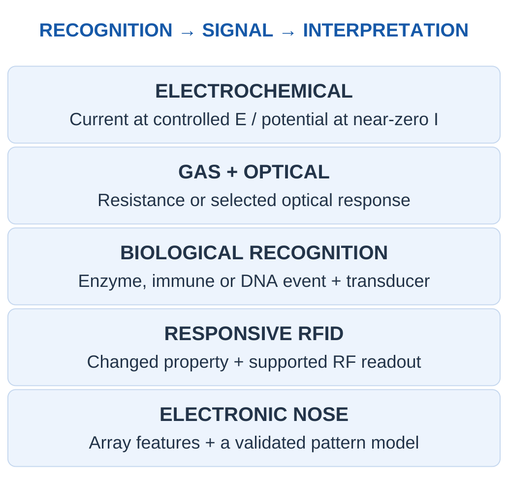
| When You See… | Complete the Explanation With… |
|---|---|
| An electrode | Current or potential mode and reference |
| A coated sensing film | Interaction, changed property and calibration |
| A biological probe | Recognition event and transducer |
| An RFID tag | Responsive interface beyond identification |
| An array pattern | Feature definition, classes and validation |
Final Check
Name the analyte and quantity, explain recognition and transduction, label current/ion/light paths correctly, preserve units and preparation factors, and qualify every result by its calibration and sample conditions.
Key Idea: A Fitted Result Needs an Independent Question
A calibration line reproducing its own fitted standards is a useful arithmetic check. An independent check sample tests a different part of the measurement claim. Repeating the same fitted points cannot alone establish selectivity, matrix transfer or later sensor stability.
Study Resources
Use these Applied Chemistry for Smart Systems Unit 3 Notes alongside the supplied figures and worked solutions. Revisit calibration assumptions, units, controls and limitations after each calculation.
These Applied Chemistry for Smart Systems Unit 3 Notes connect chemical recognition with electrochemical, optical, gas, biological and RFID sensing methods.
For revision, use the Applied Chemistry for Smart Systems Unit 3 Notes formula guide, all 39 worked examples and the complete short and examination answers.
More study material: https://www.notesgallery.com
University website: https://aktu.ac.in