Course Code: BP101T
Unit V Overview
Course: BP101T. Unit V: Data Visualization with Matplotlib.
A scientific graph communicates a numerical pattern, its units and its limitations. Matplotlib provides plotting tools for lines, histograms, scatter plots and box plots. This unit explains both code and interpretation.
Topics Covered – Syllabus Coverage
| Required topic | Coverage |
|---|---|
| Introduction to Matplotlib | Sections 5.1-5.2 |
| Line plots | Sections 5.3-5.4 |
| Histograms | Sections 5.5-5.6 |
| Scatter plots | Sections 5.7-5.8 |
| Box plots | Sections 5.9-5.10 |
| Axes, titles and legends | Sections 5.11-5.12 |
| Oral / IV concentration-time curves | Sections 5.13-5.14 |
| ADR reporting rates across drugs | Sections 5.15-5.16 |
| Dissolution profiles and scientific interpretation | Sections 5.17-5.20 |
Learning outcomes Choose an appropriate chart; draw labelled axes and legends; distinguish observations from connecting lines; explain distribution summaries; interpret pharmaceutical graphs without overstating causation or clinical significance.
Teaching datasets
Every dataset and plot in this unit is synthetic. The plotted values are selected to demonstrate graph construction and reading. They do not describe a marketed drug, validated assay or real clinical study.
- Use units in axis labels and meaningful, factual titles.
- Show observed points when a line connects sampled values.
- Do not interpret report counts as incidence without an appropriate denominator.
- A box-plot flagged point is not automatically an error.
Prerequisites
Revise arrays, DataFrames, data cleaning and aggregation. The same checks needed for a table remain necessary when that table becomes a graph.
5.1 Matplotlib installation and first plot
Matplotlib is a Python plotting library. pyplot provides plotting functions, usually imported as plt. The recommended Figure/Axes approach keeps the graph container separate from the plotting area.
Official installation guide: Install Matplotlib.
Set up – step by step
- Step 1: select the project’s Python interpreter or notebook kernel.
- Step 2: run python -m pip install matplotlib in that environment.
- Step 3: run import matplotlib.pyplot as plt to verify import.
- Step 4: create a Figure and Axes, supply the values, label the axes and display the result.
The script creates three plotted observations. In a desktop environment, show() normally opens a graph window. In a notebook, the graph generally appears with the executed cell. Display behaviour depends on the backend.
Roles of Figure and Axes
| Object | Role | Typical action |
|---|---|---|
| Figure | Whole drawing container | Save image; arrange panels |
| Axes | One plotting area | Plot data; label x and y |
| Axis | Ticks and coordinate scale | Set tick locations and formatting |
| Artist | Visible plot element | Line, marker, text or legend |
Memory trick Figure is the sheet; Axes is the graph area. An Axes object contains both x and y axes.
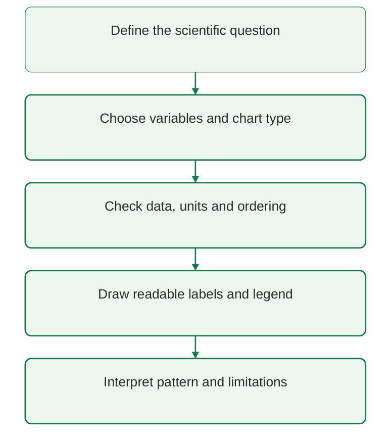
Diagram labels: Define the scientific question; choose variables and chart type; check data, units and ordering; draw readable labels and legend; interpret pattern and limitations.
Diagram explanation: Choosing a chart comes after defining what is being compared. Clear appearance is useful only when the plotted quantities and interpretation are correct.
5.2 Choosing the correct graph
The best chart depends on the variable types and the analytical question. A line communicates ordered progression; a histogram communicates a distribution; a scatter plot communicates paired values; a box plot summarises distributions.
| Graph | Data relationship | Appropriate question |
|---|---|---|
| Line | Ordered x with paired y | How does concentration change over time? |
| Histogram | One numeric variable | How are readings distributed? |
| Scatter | Two numeric variables | Do paired measurements show a pattern? |
| Box plot | Numeric variable by group | How do group distributions differ? |
| Bar, supplementary | Categories and counts/rates | How many reports or reports per exposure? |
Do not substitute chart types blindly
- Connecting unrelated categories with a line suggests a progression that may not exist.
- A histogram has numeric intervals; a bar chart has categories.
- A scatter plot preserves paired observations rather than binning them.
- A box plot hides individual details; add points or counts when that detail matters.
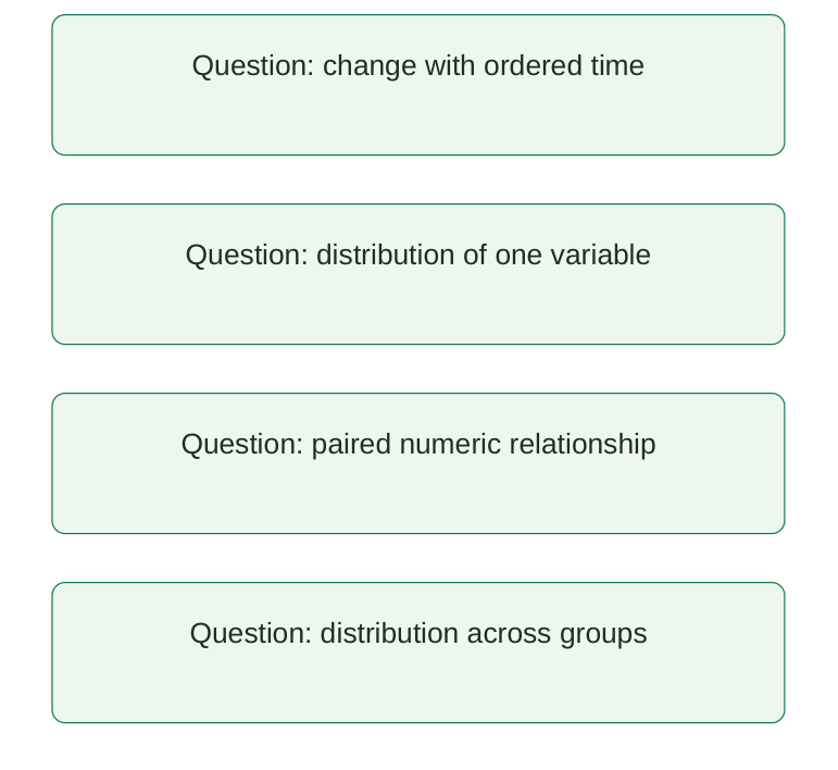
Diagram labels: Change with ordered time; distribution of one variable; paired numeric relationship; distribution across groups.
Diagram explanation: These are alternative questions. Their order in the diagram does not imply that all four charts must be created for every dataset.
Preparation checks
Make sure the data represent the intended observational unit. Keep time and concentration paired, sort by time within the correct subject, preserve missingness and verify units before plotting.
Exam answer tip Explain why the chosen graph fits the variables; naming a plotting function alone is insufficient.
5.3 Line plots: ordered observations
A line plot draws y values against ordered x values and connects adjacent points. Markers distinguish the observations from the connecting line. Time is a common x variable in pharmaceutical examples.
import matplotlib.pyplot as plt time_h = [0, 1, 2, 4, 6] concentration_mg_l = [0, 5, 4, 2, 1] fig, ax = plt.subplots() ax.plot( time_h, concentration_mg_l, marker=”o”, color=”#157A49″, ) ax.set_xlabel( “Time after reference event (h)” ) ax.set_ylabel(“Concentration (mg/L)”) ax.set_title( “Synthetic concentration-time observations” ) fig.tight_layout() plt.show()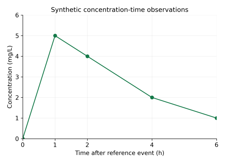
Interpretation: The largest sampled concentration is 5 mg/L at 1 h. Connecting lines guide the eye between observations; they are not measurements at every intermediate time.
Read the graph step by step
- Step 1: identify the variables and units on both axes.
- Step 2: read the coordinate of a marker rather than estimating from a smooth-looking line.
- Step 3: compare changes over stated intervals: 5 to 4 mg/L from 1 to 2 h, then 4 to 2 mg/L from 2 to 4 h.
- Step 4: state what is observed and what remains uncertain between sampled times.
Memory trick Points are observations; the line connects them.
5.4 Line ordering, multiple series and missing observations
Matplotlib connects points in the order supplied. If time values are unsorted, the line can move backwards and create a misleading pattern. Sort complete paired records rather than each variable independently.
import pandas as pd df = pd.DataFrame( { “time_h”: [2.0, 0.0, 1.0], “value”: [3.0, 0.0, 4.0], } ) df = df.sort_values(“time_h”) print(df[“time_h”].tolist()) print(df[“value”].tolist())Output
[0.0, 1.0, 2.0] [0.0, 4.0, 3.0]Two labelled series
import matplotlib.pyplot as plt time_h = [0, 1, 2] fig, ax = plt.subplots() ax.plot( time_h, [0, 4, 3], marker=”o”, label=”A” ) ax.plot( time_h, [0, 6, 5], marker=”s”, label=”B” ) ax.set_xlabel(“Time (h)”) ax.set_ylabel(“Concentration (mg/L)”) ax.legend(title=”Synthetic group”) plt.show()Use distinct markers as well as colours so the two series remain distinguishable in grayscale printing. The legend must identify exactly which line represents which group.
Missing values
import matplotlib.pyplot as plt import numpy as np fig, ax = plt.subplots() ax.plot( [0, 1, 2, 3], [0, 4, np.nan, 2], marker=”o”, ) ax.set_xlabel(“Time (h)”) ax.set_ylabel(“Concentration (mg/L)”) plt.show()NaN can break the plotted line instead of silently connecting across an unavailable measurement. Interpolation or omission changes what is being shown and must be documented.
Common error An averaged time-course curve can hide participant-level variability. State whether the plotted series is individual data or a group summary.
5.5 Histograms: frequency in numeric intervals
A histogram divides a numeric variable into bins and counts how many observations fall in each interval. It displays distribution rather than the original order of readings.
import matplotlib.pyplot as plt values = [4, 5, 5, 6, 6, 6, 7, 7, 8, 9] bins = [3.5, 5.5, 7.5, 9.5] fig, ax = plt.subplots() ax.hist( values, bins=bins, color=”#157A49″, edgecolor=”white”, ) ax.set_xlabel(“Concentration (mg/L)”) ax.set_ylabel(“Number of observations”) ax.set_title(“Synthetic readings: n = 10”) plt.show()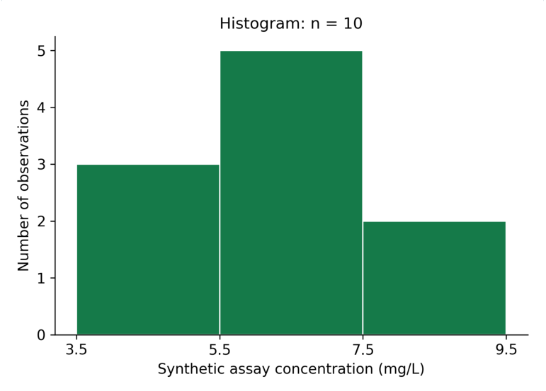
Interpretation: The bin counts are 3, 5 and 2. The total is 10 observations. The tallest bin is the middle concentration interval; it does not identify a single most frequent exact value.
| Interval | Contained values | Count |
|---|---|---|
| 3.5 to below 5.5 | 4, 5, 5 | 3 |
| 5.5 to below 7.5 | 6, 6, 6, 7, 7 | 5 |
| 7.5 to 9.5 inclusive | 8, 9 | 2 |
NumPy/Matplotlib histograms use half-open bins except the last, which includes the rightmost edge. Stating bin edges makes the classification unambiguous.
Memory trick Histogram = how many values in each interval, not a line of observations in time.
5.6 Bin choice, density and histogram interpretation
The number and width of bins affect a histogram’s appearance. Too few bins can conceal structure; too many can make a small sample look irregular. Choose bins suitable for the scale and report them.
import numpy as np values = [4, 5, 5, 6, 6, 6, 7, 7, 8, 9] counts, edges = np.histogram( values, bins=[3.5, 5.5, 7.5, 9.5] ) print(counts.tolist()) print(counts.sum())Output
[3, 5, 2] 10Count versus density
With density=False, the y-axis shows counts. With density=True, the histogram is normalised so that the sum of bin height × bin width is one. Individual density heights do not generally sum to one.
import numpy as np values = [4, 5, 5, 6, 6, 6, 7, 7, 8, 9] density, edges = np.histogram( values, bins=[3.5, 5.5, 7.5, 9.5], density=True, ) print(density.tolist()) print( float(np.sum(density * np.diff(edges))) )Output
[0.15, 0.25, 0.1] 1.0| Y-axis | What height means | Label |
|---|---|---|
| Count | Number in bin | Number of observations |
| Density | Count divided by total and bin width | Probability density |
| Relative frequency | Proportion in bin under chosen weighting | Proportion of observations |
Interpret with restraint
- Describe centre, spread, asymmetry and apparent gaps without claiming a population distribution from a tiny sample.
- Use the same bins when visually comparing groups.
- For unequal-width bins, a density display is needed if area is intended to represent proportion.
- A histogram alone does not prove normality or a statistically significant difference.
Exam point Probability is represented by area under a density histogram, not by its raw height.
5.7 Scatter plots: paired quantitative observations
A scatter plot shows a point for each paired x-y observation. It helps examine direction, curvature, spread and unusual pairs. It does not connect points in their input order.
import matplotlib.pyplot as plt prepared_mg_l = [1, 2, 3, 4, 5] response = [1.1, 1.9, 3.2, 3.8, 5.1] fig, ax = plt.subplots() ax.scatter( prepared_mg_l, response, color=”#157A49″ ) ax.set_xlabel( “Prepared concentration (mg/L)” ) ax.set_ylabel(“Response (arbitrary units)”) ax.set_title( “Synthetic calibration observations” ) plt.show()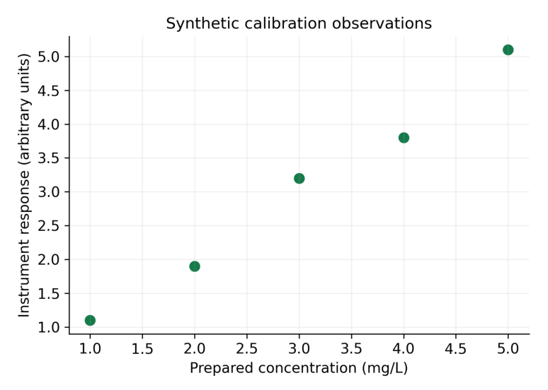
Interpretation: Response increases with the prepared concentration in these synthetic points. The plot alone does not establish linearity, method validity or a validated calibration equation.
Read paired coordinates
| Prepared concentration | Response |
|---|---|
| 1 mg/L | 1.1 arbitrary units |
| 2 mg/L | 1.9 arbitrary units |
| 3 mg/L | 3.2 arbitrary units |
| 4 mg/L | 3.8 arbitrary units |
| 5 mg/L | 5.1 arbitrary units |
A point’s horizontal and vertical coordinates belong to the same observation. Swapping or independently sorting one variable breaks that pairing.
Memory trick One observation, one coordinate pair, one point.
5.8 Scatter patterns and the limits of association
A rising scatter pattern suggests a positive association; a falling pattern suggests a negative association. A curved or widely scattered pattern requires a more careful description than “linear”.
Association is not causation
- An observed relationship can reflect a third variable, selection or repeated-measure structure.
- A visual trend does not provide a significance test or an uncertainty interval.
- A fitted line is a model result and should be labelled separately from observed points.
- Extrapolating beyond the observed range requires additional assumptions.
Output
Slope: 0.99 Intercept: 0.05The fitted slope is 0.99 response units per mg/L, with intercept 0.05 response units. This extension demonstrates a fitted model, not assay validation. Residuals, replication, working range and appropriate method criteria need separate assessment.
Readable markers
import matplotlib.pyplot as plt fig, ax = plt.subplots() ax.scatter( [1, 2, 3], [1.1, 1.9, 3.2], s=50, alpha=0.8, marker=”o”, ) ax.set_xlabel(“Concentration (mg/L)”) ax.set_ylabel(“Response (arbitrary units)”) plt.show()Marker size and transparency can improve visibility when points overlap. These choices should not imply a third variable unless size or colour is deliberately mapped and explained.
Exam distinction A correlation pattern describes association. A causal conclusion needs an appropriate design and evidence beyond the graph.
5.9 Box plots: median, quartiles and whiskers
A box plot summarises a numeric distribution. The box runs from the first quartile Q1 to the third quartile Q3; the line inside shows the median. The interquartile range is IQR = Q3 − Q1.
import matplotlib.pyplot as plt values = [1, 2, 3, 4, 5, 6, 7, 8, 20] fig, ax = plt.subplots() ax.boxplot( [values], whis=1.5, patch_artist=True ) ax.set_xticks([1], [“Batch A”]) ax.set_ylabel(“Synthetic reading (mg/L)”) ax.set_title(“Box plot: 1.5 x IQR rule”) plt.show()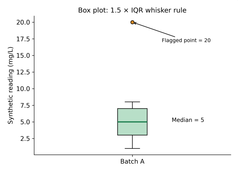
Interpretation: Q1 = 3, median = 5 and Q3 = 7 under the stated percentile convention. The upper fence is 13; the upper whisker ends at 8, the largest observed value within the fence. The value 20 is plotted separately.
| Element | Value | Meaning |
|---|---|---|
| Q1 | 3 | Lower quartile |
| Median | 5 | Middle observation |
| Q3 | 7 | Upper quartile |
| IQR | 4 | 7 minus 3 |
| Fences | -3 and 13 | Q1 – 1.5 IQR; Q3 + 1.5 IQR |
| Whisker endpoints | 1 and 8 | Observed values within fences |
| Flagged point | 20 | Outside upper fence |
Important correction Whiskers are not automatically the minimum and maximum. Under the default 1.5 IQR rule, values beyond the fences appear as separate points.
5.10 Comparing box plots and checking flagged points
Box plots can compare the median and spread of several groups. Show sample sizes because the visual summary does not communicate the reliability of small groups by itself.
import matplotlib.pyplot as plt a = [4, 5, 5, 6, 7] b = [3, 4, 6, 8, 9] fig, ax = plt.subplots() ax.boxplot([a, b], patch_artist=True) ax.set_xticks( [1, 2], [“A (n=5)”, “B (n=5)”] ) ax.set_ylabel( “Synthetic concentration (mg/L)” ) ax.set_title(“Teaching batch distributions”) plt.show()Both groups have five observations. A difference in box width or whisker extent is a descriptive pattern; it is not a significance test. Overlap or non-overlap of ordinary boxes does not establish a particular p value.
Review an unusual observation
- Step 1: identify the flagged coordinate and its source record.
- Step 2: check transcription, units and instrument or procedural context.
- Step 3: apply a predefined exclusion policy if an actual error is established.
- Step 4: retain a legitimate extreme observation; do not remove it solely because the graph flags it.
- Step 5: report any exclusion and its effect on the summary.
| Graph feature | Permitted statement | Overstatement to avoid |
|---|---|---|
| Different medians | Observed centres differ | Treatment is superior |
| Long whisker | Values spread within rule | All values are errors |
| Separate point | Outside plotting fence | Must be deleted |
Memory trick Flag means investigate; it does not mean delete.
5.11 Axis labels, ticks, scales and limits
An axis label states the variable and unit. Ticks show numeric reference points. Axis limits define the displayed range. A clear graph normally needs all three.
import matplotlib.pyplot as plt fig, ax = plt.subplots() ax.plot( [0, 1, 2, 4], [0, 5, 4, 2], marker=”o” ) ax.set_xlabel(“Time (h)”) ax.set_ylabel(“Concentration (mg/L)”) ax.set_xticks([0, 1, 2, 4]) ax.set_xlim(0, 4) ax.set_ylim(0, 6) ax.grid(alpha=0.2) plt.show()Linear and logarithmic scales
A linear scale uses equal distances for equal differences. A logarithmic scale uses equal distances for equal ratios. A log y-axis can help inspect exponential decline but cannot display zero or negative values on the ordinary log scale.
import matplotlib.pyplot as plt fig, ax = plt.subplots() ax.plot( [0, 1, 2, 3], [8, 4, 2, 1], marker=”o” ) ax.set_yscale(“log”) ax.set_xlabel(“Time (h)”) ax.set_ylabel( “Concentration (mg/L), log scale” ) plt.show()| Design choice | Check |
|---|---|
| Units | Use the same unit convention across compared curves |
| Tick intervals | Show enough numeric points to read coordinates |
| Log scale | Identify it and handle non-positive observations |
| Limits | Do not hide relevant points |
| Bar baseline | Usually start at zero for count/rate bars |
A truncated vertical range can exaggerate small differences. It may be useful for a specialised line plot if clearly labelled, but it should not conceal the scale or change the meaning of bar heights.
Exam point Scale affects appearance, not the underlying data. Identify it before interpreting a slope or difference.
5.12 Titles, legends, annotations and print quality
A title states what is shown without asserting an unproven conclusion. A legend maps symbols to series. An annotation points to a specific feature with a factual description.
import matplotlib.pyplot as plt fig, ax = plt.subplots(figsize=(6, 4)) ax.plot( [0, 1, 2], [0, 5, 4], marker=”o”, label=”Synthetic group A”, ) ax.set_xlabel(“Time (h)”) ax.set_ylabel(“Concentration (mg/L)”) ax.set_title(“Observed teaching values”) ax.legend() ax.annotate( “Sampled maximum”, xy=(1, 5), xytext=(1.1, 5.4), arrowprops={“arrowstyle”: “->”}, ) fig.tight_layout() plt.show()Choose restrained styling
- Use high-contrast text and avoid relying on colour alone.
- Use different markers or line patterns for compared series.
- Keep the legend from covering observations.
- Use a faint grid when it helps coordinate reading; avoid decorative clutter.
- Choose fonts readable at the graph’s final printed size.
Saving for notes
fig.savefig( “plot.png”, dpi=300, bbox_inches=”tight” ) fig.savefig(“plot.pdf”, bbox_inches=”tight”)These commands assume fig already refers to the intended Figure. PNG is a raster image; a PDF can preserve vector lines and text. Save the figure before closing it, and inspect the actual inserted size in the notes.
| Export setting | Purpose |
|---|---|
| dpi=300 | Detailed raster for print |
| bbox_inches=”tight” | Include labels within a fitted boundary |
| tight_layout() | Reduce label collisions |
| PDF / SVG | Preserve suitable vector elements |
Memory trick Title identifies; axes quantify; legend distinguishes; caption explains.
5.13 Oral and IV concentration-time curves
A concentration-time plot places elapsed time after administration on x and measured concentration on y. Route, formulation, dose, sampling design and analysis population affect the pattern, so comparable axes do not imply a valid route comparison.
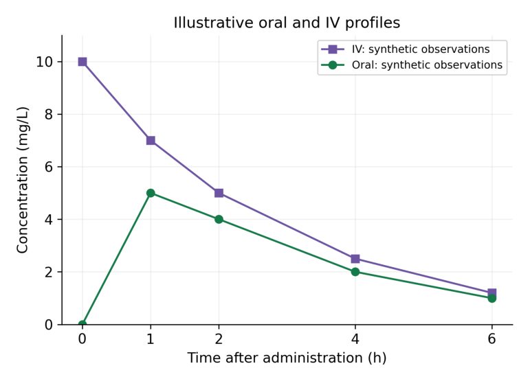
Interpretation: The IV teaching series begins at a non-zero concentration, whereas the oral teaching series rises from zero to a sampled maximum at 1 h and then falls. These illustrative values are not a fitted model or a claim about every drug or IV administration.
| Time (h) | Oral (mg/L) | IV (mg/L) |
|---|---|---|
| 0 | 0 | 10 |
| 1 | 5 | 7 |
| 2 | 4 | 5 |
| 4 | 2 | 2.5 |
| 6 | 1 | 1.2 |
An IV bolus can show an early high concentration followed by decline, but an IV infusion has a different input pattern. “IV” alone does not specify bolus versus infusion. The figure is labelled as a simplified teaching comparison.
Code structure
import matplotlib.pyplot as plt t = [0, 1, 2, 4, 6] oral = [0, 5, 4, 2, 1] iv = [10, 7, 5, 2.5, 1.2] fig, ax = plt.subplots() ax.plot( t, oral, marker=”o”, label=”Oral: synthetic”, ) ax.plot( t, iv, marker=”s”, label=”IV: synthetic” ) ax.set_xlabel( “Time after administration (h)” ) ax.set_ylabel(“Concentration (mg/L)”) ax.legend() plt.show()Interpretation limit Do not infer bioavailability, clearance, therapeutic efficacy or a recommended dose from these invented curves.
5.14 Observed maxima, sampling and model distinctions
For an observed series, the largest recorded concentration is the sampled maximum. Its time is the time of that observation. Sparse sampling may miss the true continuous-time peak.
import numpy as np t = np.array([0.0, 1.0, 2.0, 4.0, 6.0]) c = np.array([0.0, 5.0, 4.0, 2.0, 1.0]) index = np.argmax(c) print(c[index], t[index])Output
5.0 1.0The result identifies 5 mg/L at 1 h among sampled points. If the curve peaks at 0.8 h between measurements, this dataset cannot reveal that exact peak from observations alone.
Observation versus model
| Plot element | What it represents | Required explanation |
|---|---|---|
| Markers | Recorded observations | Sample size and measurement units |
| Connecting line | Visual connection | Not continuous measurement |
| Fitted curve | Model-predicted values | Model and estimation method |
| Error bars | Specified uncertainty or variability | SD, SE or CI and n |
An error bar labelled SD describes spread; an SE describes precision of an estimated mean under assumptions; a CI describes an interval from a stated method. These should not be used interchangeably.
Repeated measures
- Keep each subject’s time-concentration observations together.
- Do not connect the last point of one participant to the first point of another.
- State whether a curve is individual data or a summary at common times.
- A group mean profile can conceal variability and missing observations.
Faculty question Ask what extra information would be needed to estimate exposure or compare routes scientifically: sampling adequacy, authorised regimen, design, units and an appropriate analytical method.
5.15 ADR counts: plot what the table contains
A categorical bar chart is a useful supplementary plot for submitted report counts across drugs. Count bars must be labelled as counts; they are not automatically reporting rates or clinical risks.
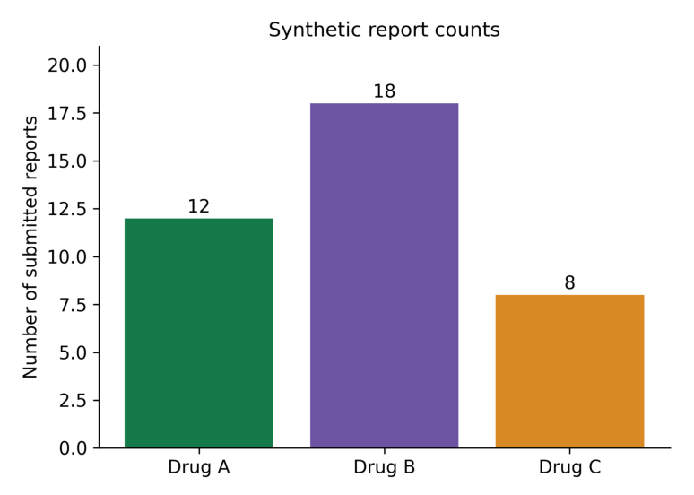
Interpretation: Drug B has the most submitted reports in this invented table: 18 versus 12 and 8. Without a suitable exposure denominator and comparable ascertainment, this does not imply that Drug B has the greatest event risk.
import matplotlib.pyplot as plt drugs = [“Drug A”, “Drug B”, “Drug C”] counts = [12, 18, 8] fig, ax = plt.subplots() ax.bar(drugs, counts) ax.set_ylabel(“Number of submitted reports”) ax.set_title(“Synthetic report counts”) ax.set_ylim(0, 21) plt.show()Why counts alone cannot estimate incidence
- The number of people exposed may differ across drugs.
- Reporting is influenced by awareness, underreporting and follow-up.
- Multiple reports or event rows may refer to the same case.
- A report does not by itself establish a causal drug-event relationship.
| Visible fact | Unsupported inference |
|---|---|
| 18 reports for Drug B | Drug B is clinically more dangerous |
| Count rises over time | True incidence necessarily rose |
| More serious reports | Higher patient-level serious-event probability |
Critical rule For spontaneous reports, use report counts or clearly defined report proportions. Incidence requires an appropriate at-risk denominator and ascertainment design.
5.16 Reporting rates with an explicitly supplied denominator
A reporting metric can be calculated when a defined teaching cohort supplies both reports and exposed participants over a stated period. Label the denominator and multiplier explicitly. This does not automatically convert reports into confirmed incident ADR cases.
| Group | Reports | Exposed participants |
|---|---|---|
| Drug A | 12 | 1,000 |
| Drug B | 18 | 2,000 |
| Drug C | 8 | 500 |
Output
[12.0, 9.0, 16.0]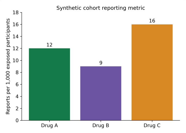
Interpretation: After this normalisation, the reporting metrics are 12, 9 and 16 per 1,000. Their order differs from the raw counts. The measure remains reports per exposed participants under the stated design, not an automatically validated incidence rate.
Stepwise calculation
- Step 1: define the reporting period and how reports and exposed people were counted.
- Step 2: confirm all denominators are positive and refer to comparable groups.
- Step 3: calculate reports / exposed participants × 1,000.
- Step 4: label the axis “Reports per 1,000 exposed participants”.
- Step 5: discuss repeated reports, case confirmation and ascertainment limitations.
A rate per person-time uses a different denominator, such as person-years. A percentage of reports uses all eligible reports as its denominator. These quantities must not share one ambiguous “ADR rate” label.
Memory trick Numerator, denominator, period and multiplier: state all four.
5.17 Dissolution profiles
A dissolution profile commonly plots cumulative percentage released against sampling time. The exact test method, medium, apparatus, conditions and calculation rule belong to the experiment’s documentation.
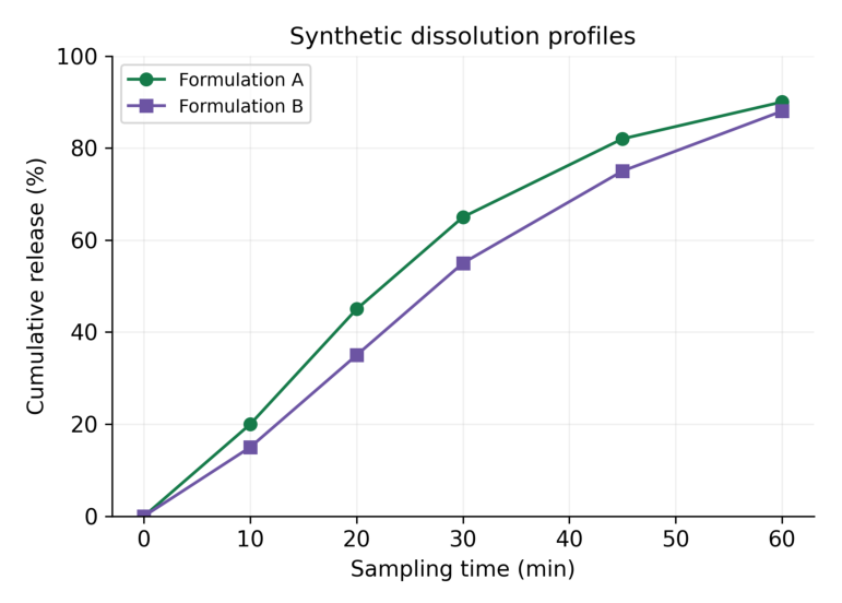
Interpretation: Both teaching series rise with time. Formulation A shows greater cumulative release at the sampled intermediate times. The plot alone does not establish pharmacopoeial compliance, equivalence or superiority.
| Time (min) | A release (%) | B release (%) |
|---|---|---|
| 0 | 0 | 0 |
| 10 | 20 | 15 |
| 20 | 45 | 35 |
| 30 | 65 | 55 |
| 45 | 82 | 75 |
| 60 | 90 | 88 |
Scientific caution The values are invented for plotting. Do not use them as an acceptance standard. Percentage released must be calculated by the validated procedure, including any applicable sampling corrections.
5.18 Comparing dissolution and group summaries
A line comparison describes observed profiles. It does not provide a statistical or regulatory similarity decision by itself. Such a decision requires the relevant method, design and acceptance criteria.
Read one interval accurately
At 30 minutes, teaching A is 65% and B is 55%. The difference is 10 percentage points. Saying “10% higher” is ambiguous: relative to 55%, the increase is about 18.18%.
a = 65 b = 55 print(a – b) print(f”{100*(a-b)/b:.2f}%”)Output
10 18.18%| Quantity | Calculation | Meaning |
|---|---|---|
| Percentage-point difference | 65 – 55 = 10 | Difference on percentage scale |
| Relative percentage difference | 100 × (65 – 55) / 55 | Increase relative to B |
| Final sampled release | 90% and 88% at 60 min | Recorded endpoint values |
Replicate profiles
- State whether each point is an individual vessel or the mean of replicates.
- Report the number of replicates and what any error bars represent.
- Keep sampling times and measurements paired.
- Do not remove a low replicate just because it reduces the mean.
A visually smooth curve can be produced from sparse points, but smoothing introduces a method beyond raw plotting. If used, label the method and retain the observed markers.
Exam point A graph may show a difference. Its clinical, experimental or regulatory importance needs evidence beyond appearance.
5.19 Scientific interpretation and misleading graphs
A good interpretation distinguishes a visible pattern from an inference. Begin with what was measured, describe the pattern, then state the limitations that affect the conclusion.
| Graph | Descriptive observation | Further evidence needed |
|---|---|---|
| Line | Concentration decreases over sampled interval | Model for elimination inference |
| Histogram | Most values lie in middle bins | Larger sample / distribution assessment |
| Scatter | Response rises with concentration | Validation and uncertainty analysis |
| Box plot | Group medians and spreads differ | Appropriate comparative analysis |
| Report bars | Counts or defined metrics differ | Comparable denominator and ascertainment |
Common distortions
- Mismatched units: comparing mg/L with µg/mL requires recognising that 1 mg/L equals 1 µg/mL; mg/mL is a different scale.
- Reordered measurements: independently sorting x and y destroys pairing.
- Hidden missing values: a continuous line may imply observations where none exist.
- Truncated count bars: a non-zero baseline can exaggerate differences.
- Undefined error bars: the viewer cannot tell spread from precision.
- Unstated denominator: report counts masquerade as patient incidence.
Interpretation template
A clear graph statement In the stated synthetic dataset, the plotted quantity changed from X to Y over the specified interval. This describes observed values; the graph does not by itself establish causation, significance or clinical suitability. Use this structure with concrete numbers and units. Avoid writing a conclusion that is stronger than the design and the plotted information support.
5.20 Complete plotting workflow and troubleshooting
Stepwise production
- Step 1: import the dataset and verify field names, units and row meaning.
- Step 2: check missingness, finite values, pairing and order.
- Step 3: choose the chart from the scientific question.
- Step 4: create Figure and Axes and plot the correct fields.
- Step 5: label axes, numerical ticks, title and legend.
- Step 6: save at the intended print size and inspect clipping or overlaps.
- Step 7: write a caption stating data origin and the interpretation limit.
| Problem | Likely reason | Action |
|---|---|---|
| No plot window | Backend / notebook display context | Check environment; save and inspect |
| x and y length error | Unpaired arrays | Validate lengths and record alignment |
| Unordered zigzag | Input times unsorted | Sort complete records |
| Labels cut off | Insufficient figure boundary | tight_layout and fitted export |
| Log-scale issue | Zero or negative y values | Choose appropriate scale and policy |
Memory trick Check data first, styling second. A attractive graph of wrongly paired values is still wrong.
5.21 Quick revision
| Graph or tool | Essential recall |
|---|---|
| Line | Ordered progression; markers are observations |
| Histogram | Distribution within numeric bins |
| Scatter | Paired numeric coordinates |
| Box plot | Median, quartiles and declared whisker rule |
| Figure / Axes | Container / plotting area |
| xlabel / ylabel | Variable plus unit |
| Legend | Identify series exactly |
| Density histogram | Area sums to one |
| Log scale | Positive values; equal ratios |
| Sampled maximum | Largest recorded point, not necessarily true peak |
| ADR metric | State numerator and denominator |
| Dissolution | Cumulative release versus stated sampling time |
Checkable answers
| Question | Answer |
|---|---|
| Histogram counts 3, 5, 2: total? | 10 |
| Box data Q1=3, Q3=7: IQR? | 4 |
| Upper fence at 1.5 IQR? | 13 |
| 12 reports / 1,000 exposed × 1,000? | 12 per 1,000 |
| 18 / 2,000 × 1,000? | 9 per 1,000 |
| 65% minus 55%? | 10 percentage points |
Caption checklist
- Identify the dataset as synthetic or state its actual source in the research context.
- State variable units, group identity and what one plotted point represents.
- Explain bin rules, whisker rules or error bars where applicable.
- Describe the visible pattern without making an unsupported causal claim.
One-minute revision Question → data check → chart choice → labels → interpretation.
5.22 Possible examination questions
Short answers
- Define Matplotlib, Figure and Axes.
- Compare a line plot with a scatter plot.
- Compare a histogram with a category bar chart.
- Explain bin edges and density normalisation.
- State the box-plot components and the 1.5 IQR rule.
- Why must units appear on axes?
- What is the purpose of a legend?
- Why is a sampled peak not necessarily the true peak?
- Why are submitted reports not an incidence denominator?
- Distinguish percentage points from relative percentage change.
Long answers
- Explain graph selection and the Figure/Axes workflow with examples.
- Construct and interpret concentration-time curves for synthetic oral and IV series.
- Explain histograms, bin selection and density.
- Construct a scatter plot and discuss association versus causation.
- Explain and interpret a box plot with a labelled flagged point.
- Plot ADR reporting metrics with an explicitly stated denominator.
- Plot dissolution profiles and explain the limitations of visual comparison.
Practical problems
- Plot time 0, 1, 2 and 4 h against concentration 0, 5, 4 and 2 mg/L with markers and units.
- Create a histogram with explicit edges and confirm the sum of bin counts.
- Draw two labelled dissolution profiles with a readable legend.
- Save a 300-dpi graph and verify every label at the final inserted size.
- Explain one misleading graph choice and provide a corrected interpretation.
Expected answer quality Provide suitable data, clear code, a correctly labelled graph, a checked numeric reading and a scientifically limited interpretation. A plot without units or a stated denominator is incomplete.