
Industrial Automation and Control Unit 4 Notes cover the sensors and signal interfaces used to provide feedback to an automatic control system. The unit, Industrial Sensors and Applications, explains optical, inductive and capacitive sensing, PNP/NPN outputs, PLC interfacing, 4–20 mA current loops and conventional wired HART communication.
These notes are for AKTU B.Tech 5th Semester EE and EN students studying BEE053. Each topic connects the sensing principle with its wiring, application and PLC interpretation. Worked examples, comparison tables and examination questions support revision.
Topics Covered
| Topic | Topic |
|---|---|
| 4.1 Introduction to industrial sensors | 4.13 Digital sensor–PLC interfacing |
| 4.2 Sensor characteristics and selection | 4.14 Sensor interpretation and PLC logic |
| 4.3 Optical sensor fundamentals | 4.15 The 4–20 mA current loop |
| 4.4 Through-beam optical sensing | 4.16 Current-loop interfacing |
| 4.5 Retroreflective and diffuse sensing | 4.17 Scaling and worked examples |
| 4.6 Optical applications and maintenance | 4.18 Loop voltage budget and faults |
| 4.7 Inductive proximity sensors | 4.19 HART protocol fundamentals |
| 4.8 Inductive mounting and applications | 4.20 HART point-to-point configuration |
| 4.9 Capacitive proximity sensors | 4.21 HART multidrop configuration |
| 4.10 Capacitive level detection | 4.22 HART communication modes |
| 4.11 Comparing sensing principles | 4.23 Integrated applications and tests |
| 4.12 PNP and NPN sensor outputs | 4.24 Revision and examination practice |
4.1 Introduction to Industrial Sensors
An industrial sensor responds to a physical condition and supplies information that a control system can use. It may detect presence, position, level, pressure, temperature or another process quantity.
A PLC depends on this feedback to interpret what is happening in the machine. The sensor detects the condition; the program decides the response; an output interface and actuator perform the action.
Sensor, Transducer and Transmitter
| Element | Main function |
|---|---|
| Sensor | Responds to a physical condition |
| Transducer | Converts one physical form into another; a sensing element is often a transducer |
| Transmitter | Conditions and communicates a measured value through a usable signal |
| PLC input | Receives the field signal and converts it into stored control information |
A proximity switch normally reports presence or absence. A measuring transmitter reports a variable quantity, such as pressure over 0–10 bar. A sensor with a digital switching output is not automatically a digital communication device.
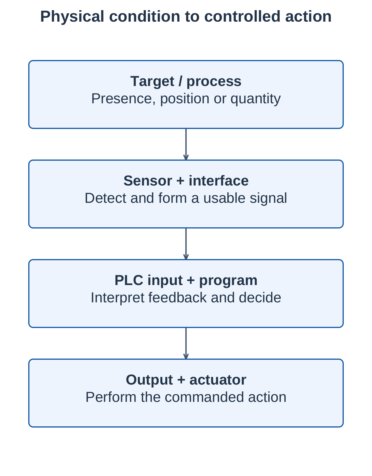
Three Questions for an Installation
- What is detected? Identify the target or process variable.
- How is it detected? Choose the suitable sensing principle.
- How is it connected? Match the output with the PLC interface.
Industrial applications include part counting, motion confirmation, product positioning, level supervision and process measurement.
4.2 Sensor Characteristics and Selection
A proximity sensor’s sensing distance describes target detection under stated conditions. A measuring sensor’s measurement range describes its specified variable interval. These are different quantities.
| Characteristic | Meaning |
|---|---|
| Sensitivity | Output change relative to input change; adjustable detection sensitivity may also be specified |
| Resolution | Smallest distinguishable input increment |
| Accuracy | Closeness to the correct value under specified conditions |
| Repeatability | Agreement between repeated measurements or switching points |
| Response time | Time required to respond to a change |
| Switching frequency | Permitted switching rate under stated conditions |
| Hysteresis | Separation between operate and release points |
| Environmental rating | Suitability for dust, water, temperature and other exposure |
Hysteresis
An approaching target can operate a proximity switch at one distance. As the target withdraws, the switch releases at a slightly greater distance. This prevents repeated switching when the target vibrates near the threshold.
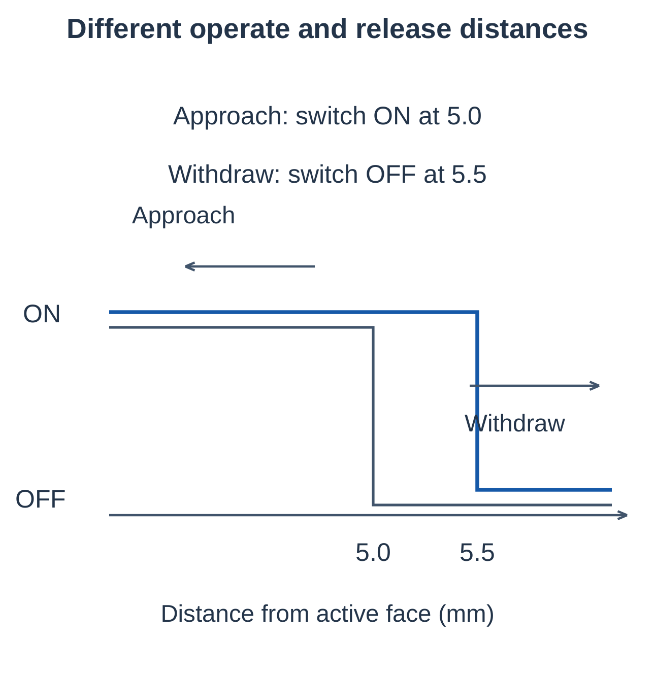
For the illustrated model:
Hysteresis = Release distance − Operate distance
Operate distance = 5.0 mm; release distance = 5.5 mm:
Hysteresis = 5.5 − 5.0 = 0.5 mm
Relative to the operate distance:
Hysteresis percentage = (0.5 / 5.0) × 100 = 10%
Use the manufacturer’s definition for a particular sensor.
Selection Steps
- Identify target material, size and motion.
- Choose the sensing principle.
- Determine operating distance and speed.
- Check mounting, surroundings and contamination.
- Match supply and output to the PLC.
- Test actual targets under normal and fault conditions.
A sufficient nominal distance alone does not establish suitability. Response speed, electrical output and target compatibility also matter.
4.3 Optical or Photoelectric Sensors
A photoelectric sensor detects a change in received light. Its arrangement determines whether the target interrupts a beam, blocks a reflected return or supplies the reflected light itself.
Construction
Typical components include:
- Light emitter.
- Lens system.
- Photodetector or receiver.
- Signal-evaluation electronics.
- Output stage.
- Protective housing.
Visible or infrared light may be used. Many sensors modulate the emitter and evaluate the corresponding received signal to reduce interference from unrelated light.
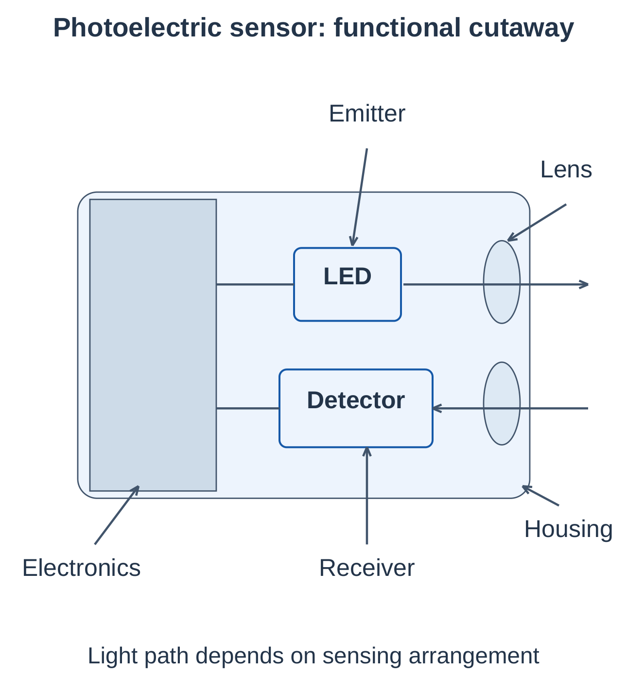
Operating Sequence
- The emitter sends light.
- The target changes the optical path.
- The receiver converts received light into an electrical signal.
- Evaluation circuitry checks the switching criterion.
- The configured output changes state.
Light-On and Dark-On Modes
| Received-light condition | Light-on output | Dark-on output |
|---|---|---|
| Sufficient light received | ON | OFF |
| Light below the switching threshold | OFF | ON |
This table assumes a simple binary light threshold. Through-beam sensing often uses dark-on to indicate an opaque target; diffuse sensing often uses light-on because the target returns light.
Light-on/dark-on describes the optical decision. PNP/NPN describes the electrical output arrangement. Confirm both separately.
4.4 Through-Beam Optical Sensing
Arrangement and Principle
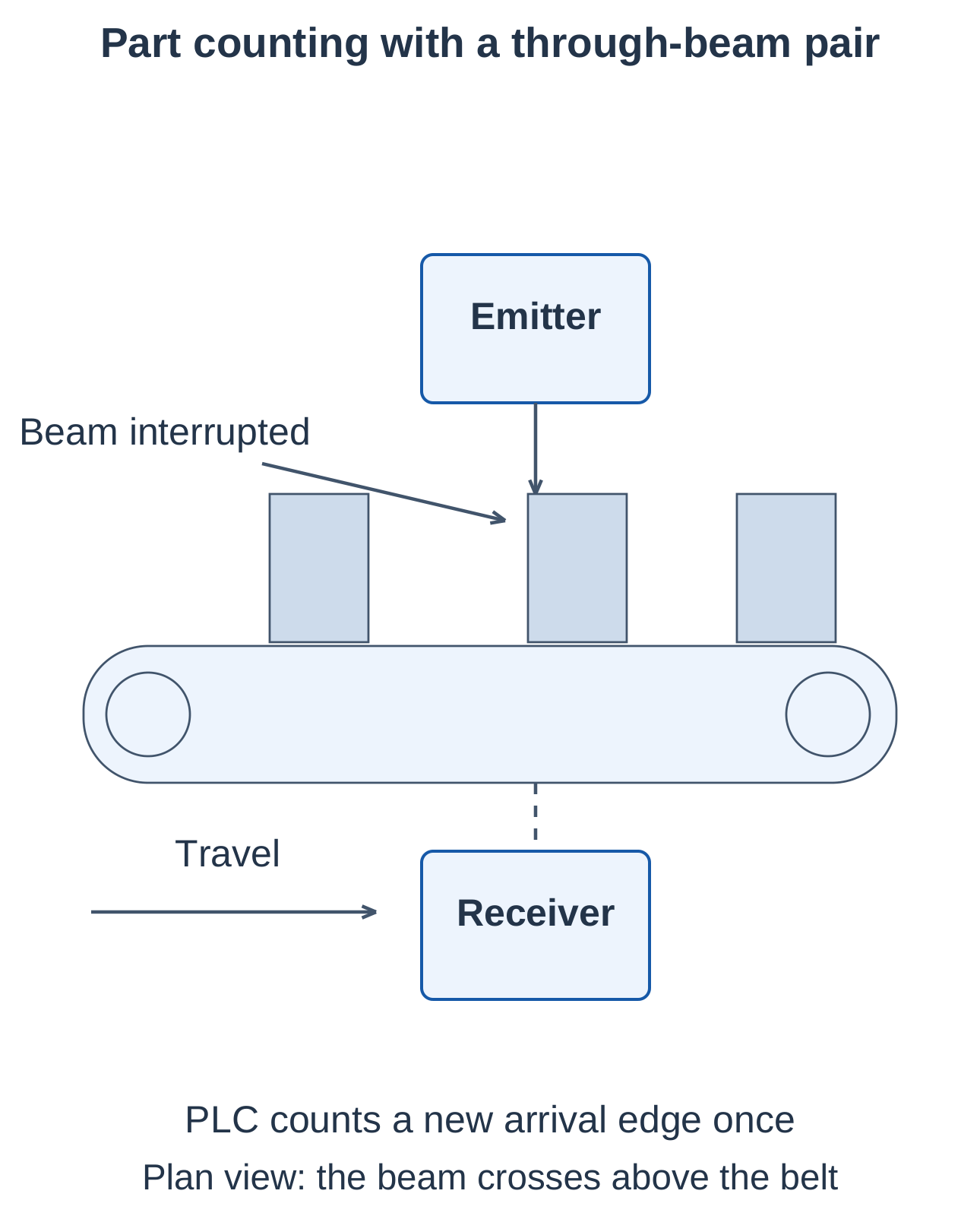
The emitter and receiver are in separate housings facing each other. An opaque target sufficiently interrupting the beam reduces the received light and changes the output.
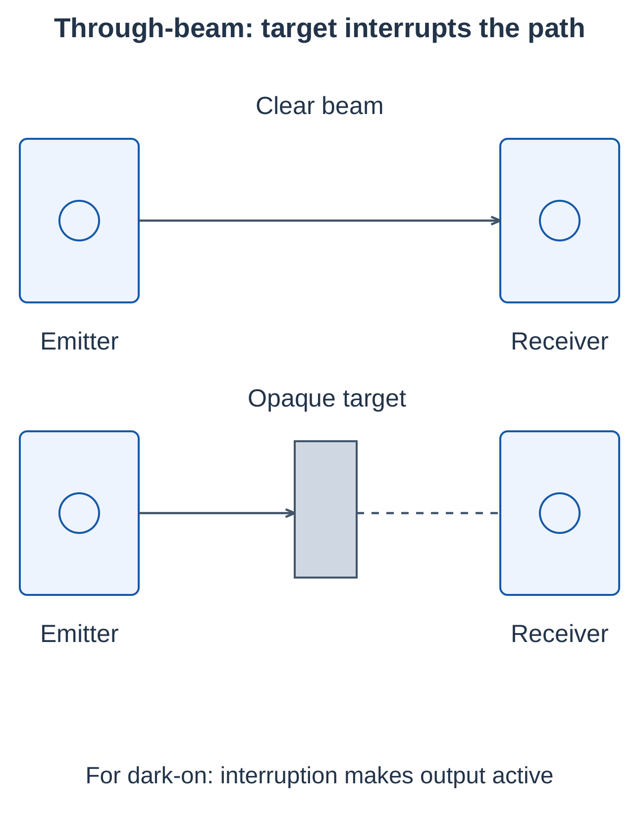
Advantages and Limitations
| Advantages | Limitations |
|---|---|
| Long operating range possible with a suitable pair | Both sides require installation and wiring |
| Reliable detection of suitable opaque targets | Alignment must be maintained |
| Colour and finish usually less influential than in diffuse sensing | Ordinary models may miss transparent targets |
| Suitable beam selection supports small-target detection | Dust and misalignment can resemble beam blockage |
Conveyor Counting
Install the beam across the travel path and define PartPresent = 1 when a target interrupts it. A rising PartPresent event increments the counter once. A part remaining in the beam for several scans should still generate one event.
Worked Speed Check
A 20 mm target moves at 1 m/s:
Occupied time = Target length / Speed
Occupied time = 0.020 / 1 = 0.020 s = 20 ms
With a 20 mm gap, the full target-and-gap cycle lasts 40 ms:
Event frequency = 1 / 0.040 = 25 Hz
The sensor, input filter and PLC sampling must resolve both occupied and clear intervals. Effective beam width also affects pulse duration.
4.5 Retroreflective and Diffuse Sensing
Retroreflective Arrangement
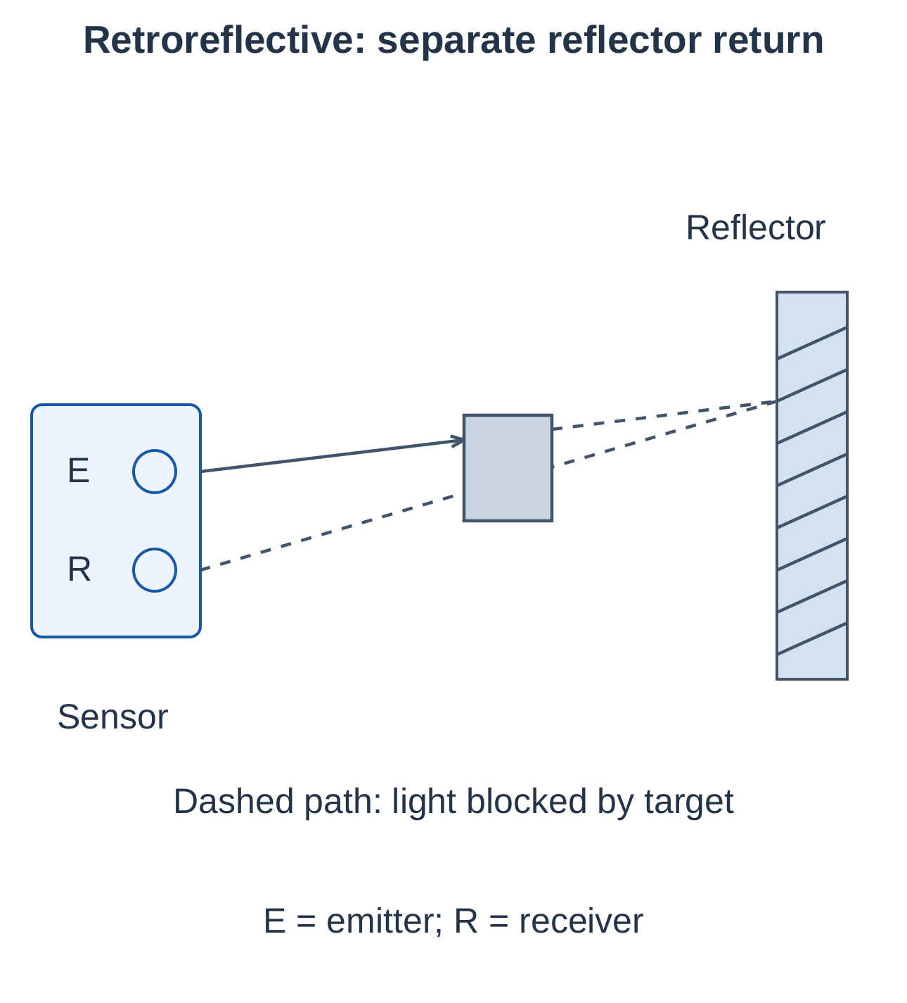
The emitter and receiver share a housing. A separate reflector returns light toward the sensor. A target is detected when it sufficiently interrupts this return path.
Only the sensor side normally needs electrical wiring, but the reflector still requires mounting and alignment. Suitable polarized arrangements help reject misleading shiny-target reflections. Transparent objects may require dedicated clear-object sensors and setup.
Diffuse-Reflective Arrangement
The emitter and receiver share a housing, and the target itself returns light. No separate reflector is used.
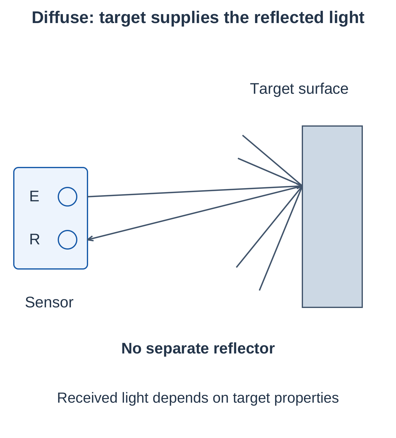
Diffuse sensing is convenient with access from one side. Performance depends on target colour, reflectivity, size, orientation and distance. A bright nearby background can produce an unwanted response.
Background Suppression
A background-suppression sensor uses a suitable distance-sensitive optical method to distinguish the intended region from more distant objects. It still has specified limits and installation requirements.
Retroreflective and Diffuse Comparison
| Feature | Retroreflective | Diffuse |
|---|---|---|
| Return source | Separate reflector | Target surface |
| Detection condition | Interruption of returned light | Sufficient target-reflected light |
| Installation | Sensor and reflector | Single sensor housing |
| Main concern | Alignment and unwanted reflections | Target reflectivity and background |
| Typical use | Conveyor presence detection | Direct detection with one-side access |
4.6 Optical Applications and Maintenance
Photoelectric sensors detect cartons, bottles, sheet edges, packages and product position. Select the arrangement for the actual product and environment.
Through-Beam and Diffuse Comparison
| Feature | Through-beam | Diffuse |
|---|---|---|
| Housings | Separate emitter and receiver | Combined emitter and receiver |
| Target effect | Blocks light | Returns light |
| Typical distance capability | Often longer in comparable applications | Often shorter and target-dependent |
| Alignment | Align both housings | Aim at the intended target |
| Important target properties | Opacity and beam interruption | Reflectivity, size and angle |
| Mounting access | Both sides | One side |
Commissioning Steps
- Secure the mounts and align the optical path.
- Verify the clear-path condition.
- Test the smallest, darkest, shiniest or most transparent expected target as applicable.
- Set sensitivity and output mode.
- Run at operating speed.
- Confirm PLC interpretation and counting behaviour.
Troubleshooting
| Symptom | Checks |
|---|---|
| Output changes without a product | Alignment, background movement, stray light and contamination |
| Dark target missed by a diffuse sensor | Signal margin, distance, angle and sensor suitability |
| Shiny target appears absent | Reflection path and reflector discrimination |
| Counts missing at high speed | Response time, filter, pulse width and sampling |
| Output remains blocked | Dirty lens, obstruction, misalignment or emitter failure |
Clean lenses and reflectors appropriately. Investigate weak signal margin before repeatedly increasing sensitivity.
4.7 Inductive Proximity Sensors
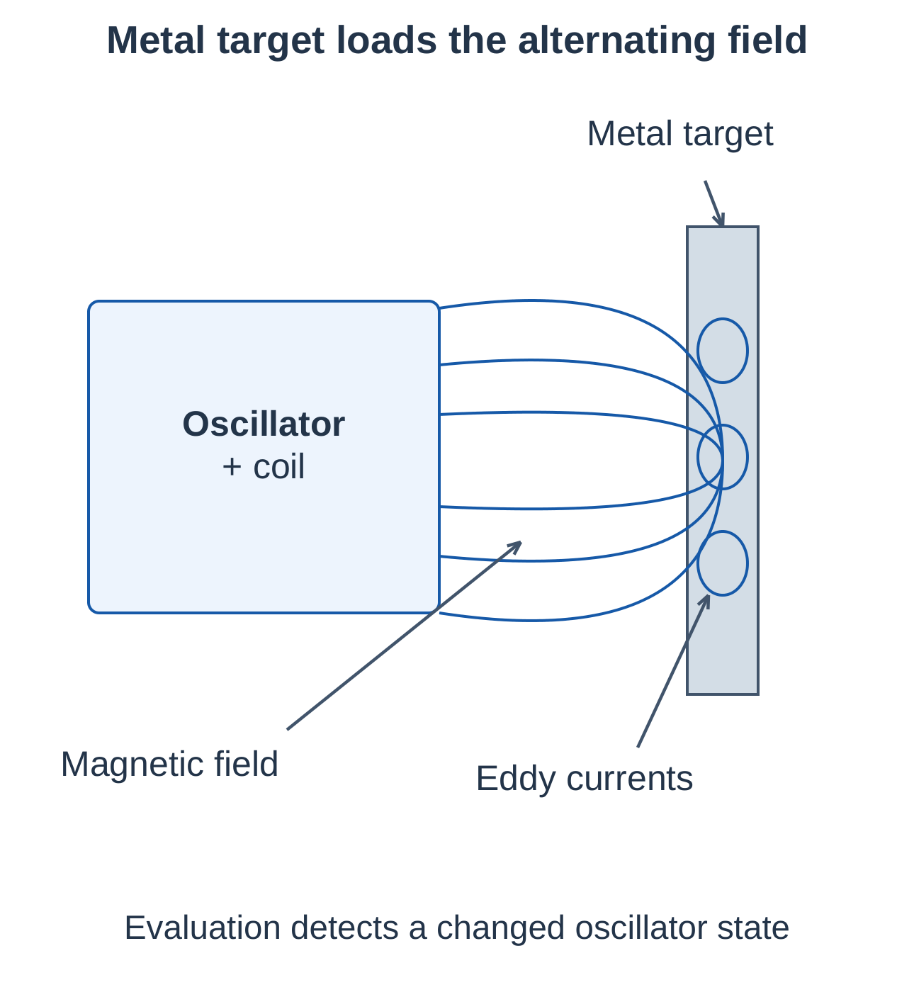
An inductive proximity sensor detects a suitable metallic target through its effect on an alternating magnetic field. It provides non-contact metal-position feedback.
Construction
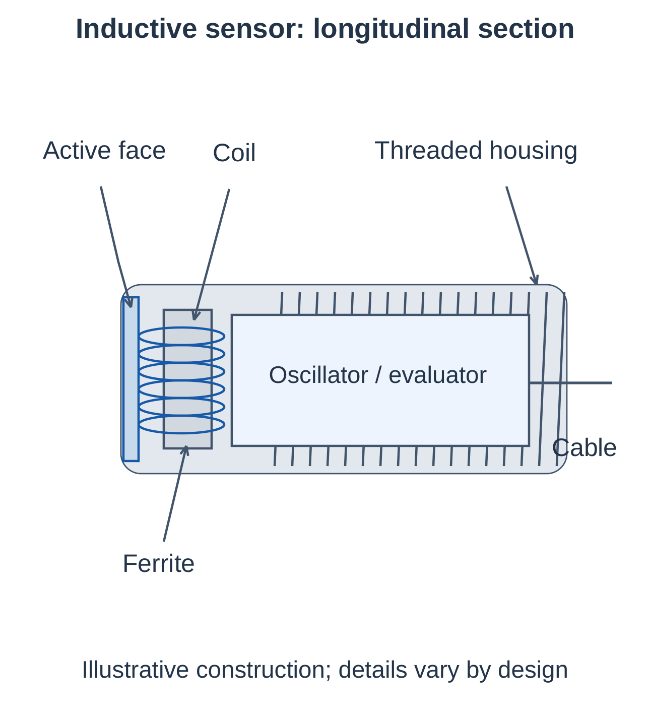
A typical sensor contains an oscillator, coil, ferrite structure, evaluation circuit and switching output. The active face directs the field toward the target.
Operating Principle
- The oscillator excites the coil.
- An alternating magnetic field forms near the active face.
- A metal target enters the field.
- Eddy currents induced in the target load the sensing circuit.
- Electronics detect the oscillator change and switch the output.
Target Material and Distance
Detection depends on target material, size, thickness, orientation and sensor design. A rated reference distance may use a specified steel target. Other metals can produce shorter ranges, while some specialized sensors provide approximately equal response for selected metals.
Worked correction example: Reference distance = 8 mm; applicable material factor = 0.5:
Estimated distance = 8 × 0.5 = 4 mm
This factor is illustrative, not universal for every aluminium target or sensor.
Inductive sensing avoids optical alignment and contact. Ordinary inductive sensors generally cannot directly detect non-metallic plastic, paper or liquid. Nearby metal can influence operation.
4.8 Inductive Mounting and Applications
Flush and Non-Flush Mounting
A flush or shielded sensor is designed for specified flush installation in surrounding metal. A non-flush or unshielded sensor normally requires free space around its active region.
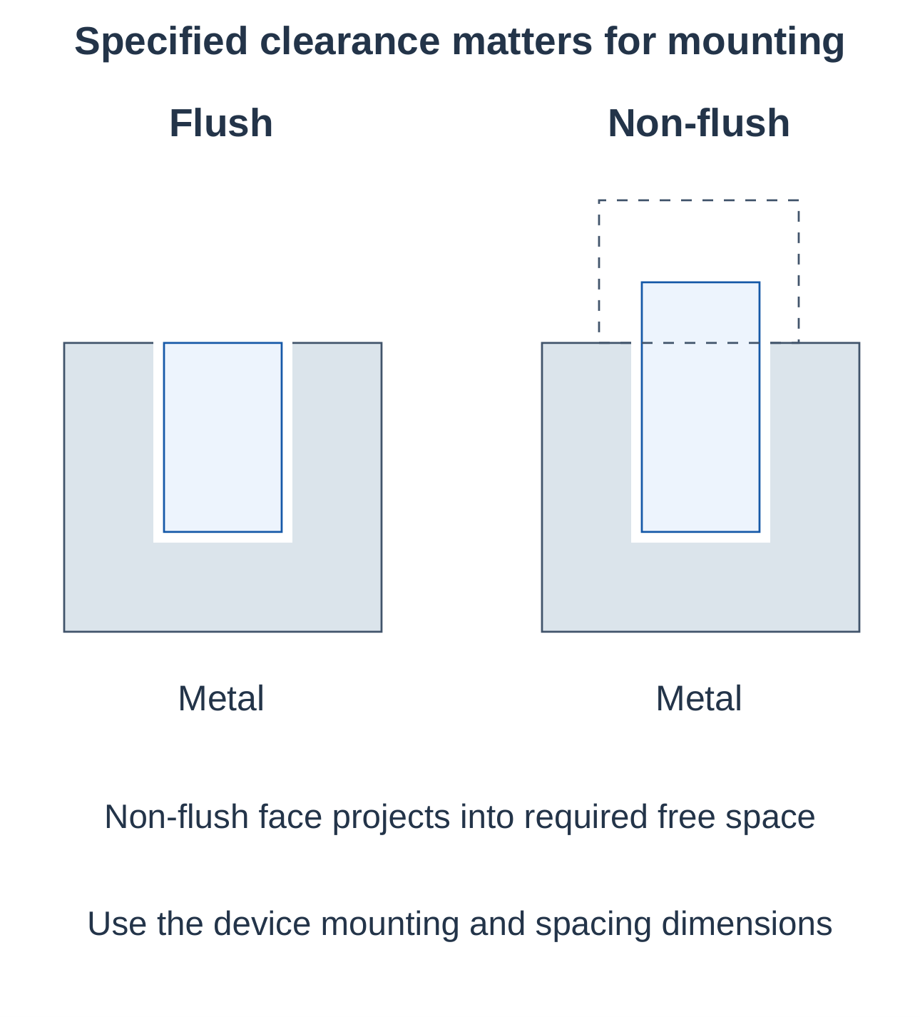
| Feature | Flush type | Non-flush type |
|---|---|---|
| Typical field | More concentrated forward field | More extensive field near the active end |
| Mounting | Specified flush mounting in metal | Specified surrounding clearance |
| Common range tendency | Often shorter for comparable size | Often longer for comparable size |
| Installation error | Incorrect face position | Nearby metal causing predamping or switching |
Use the actual mounting drawing. Adjacent sensor separation also depends on construction and operating frequency.
Applications
- Metal slide or actuator end-position confirmation.
- Gear-tooth or slot detection.
- Metal workpiece confirmation before machining.
- Metal-part counting.
- Tool-fixture presence detection.
Gear Pulse-Rate Example
A gear has 12 detectable teeth and rotates at 300 rpm:
Revolutions per second = 300 / 60 = 5
Event rate = 12 × 5 = 60 Hz
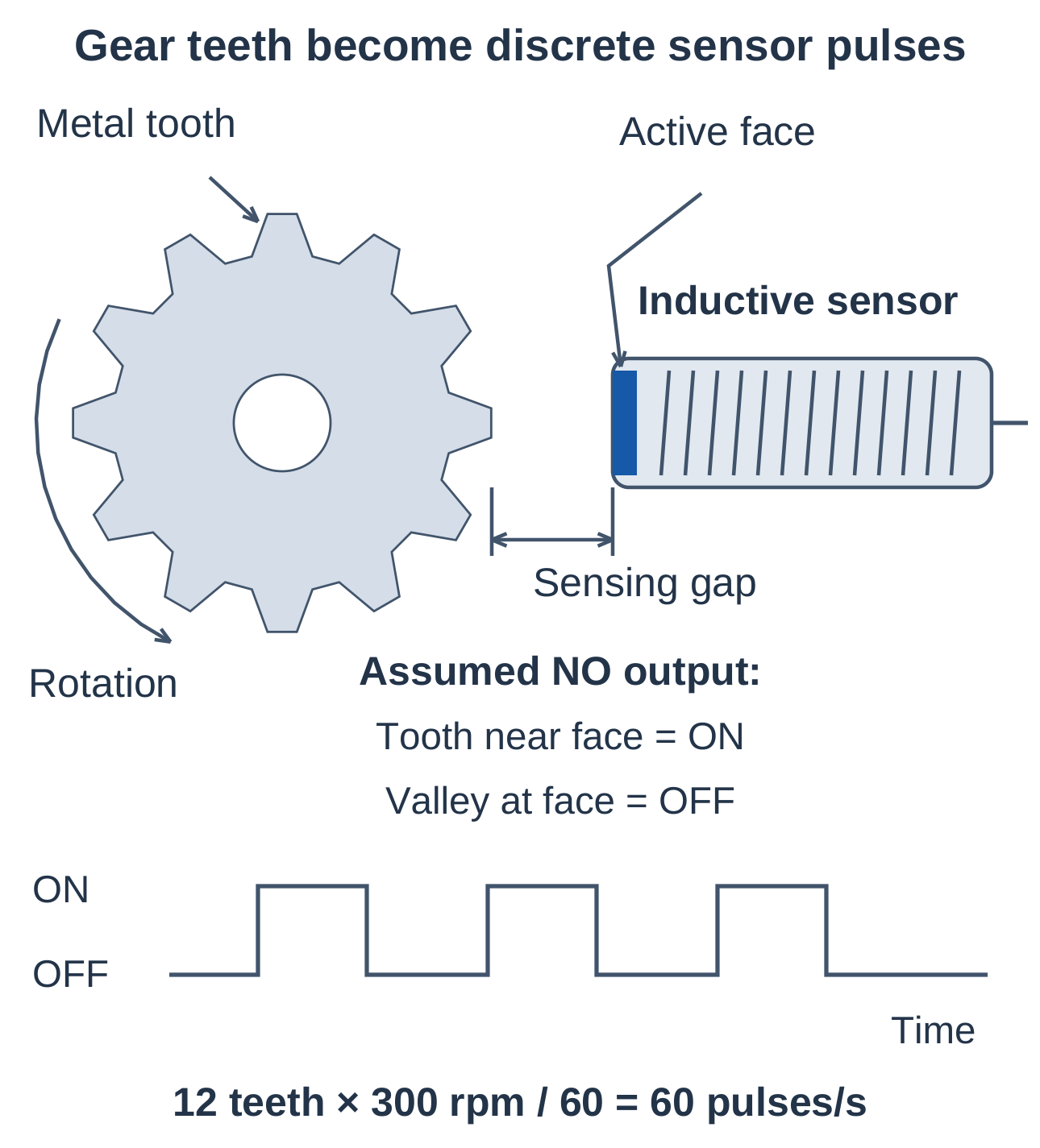
Check the actual tooth and gap durations, target runout, vibration, sensor gap, adjacent fields, cable strain and mechanical protection. A sensor’s maximum switching-frequency rating alone does not verify PLC acquisition.
4.9 Capacitive Proximity Sensors
A capacitive proximity sensor detects a change in effective capacitance caused by nearby material. Suitable targets include metals, non-metals, liquids, powders and solids.
Construction and Principle
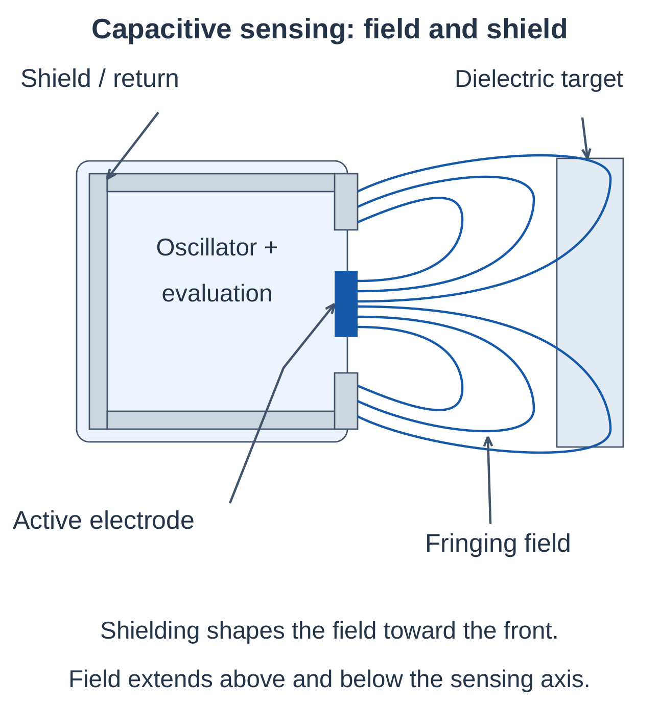
An active electrode and return or reference arrangement create an electric field. A target changes the capacitance seen by the sensing circuit.
- Establish the sensing field.
- Introduce the target.
- Detect the capacitance change.
- Compare it with the switching threshold.
- Change the configured output state.
Capacitance Relationship
For an ideal parallel-plate capacitor:
C = ε₀ εᵣ A / d
| Symbol | Meaning |
|---|---|
| C | Capacitance |
| ε₀ | Vacuum permittivity |
| εᵣ | Relative permittivity |
| A | Overlapping plate area |
| d | Plate separation |
This illustrates the influence of material and geometry. A proximity sensor uses a fringing field, so the ideal two-plate equation is not a complete sensor-distance model.
Advantages and Limitations
Capacitive sensing can detect a broader material range than ordinary inductive sensing. Suitable equipment can detect contents through a non-metallic wall.
Response can also change with humidity, deposits, moisture, composition, wall thickness and nearby objects. Test the intended material against the empty container and expected surrounding conditions.
4.10 Capacitive Level Detection
External Point-Level Sensing
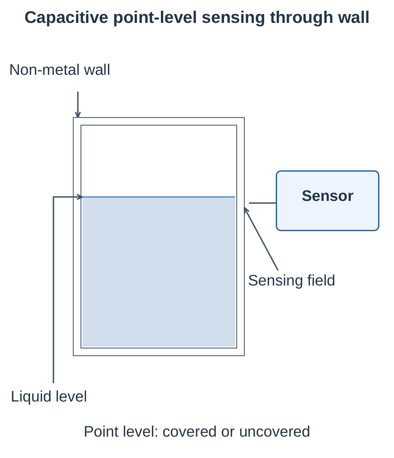
A suitable capacitive sensor can be mounted outside a non-metallic tank at a defined height. Its field passes through the wall sufficiently to detect the intended contents.
This is point-level sensing: covered or uncovered at one position. It does not automatically provide continuous percentage level.
Empty/Full Setup
- Mount at the required height.
- Check the empty or below-level state.
- Introduce the actual material to the sensing height.
- Adjust or teach the switching criterion.
- Remove the material and confirm release.
- Repeat under expected temperature, deposit and material variations.
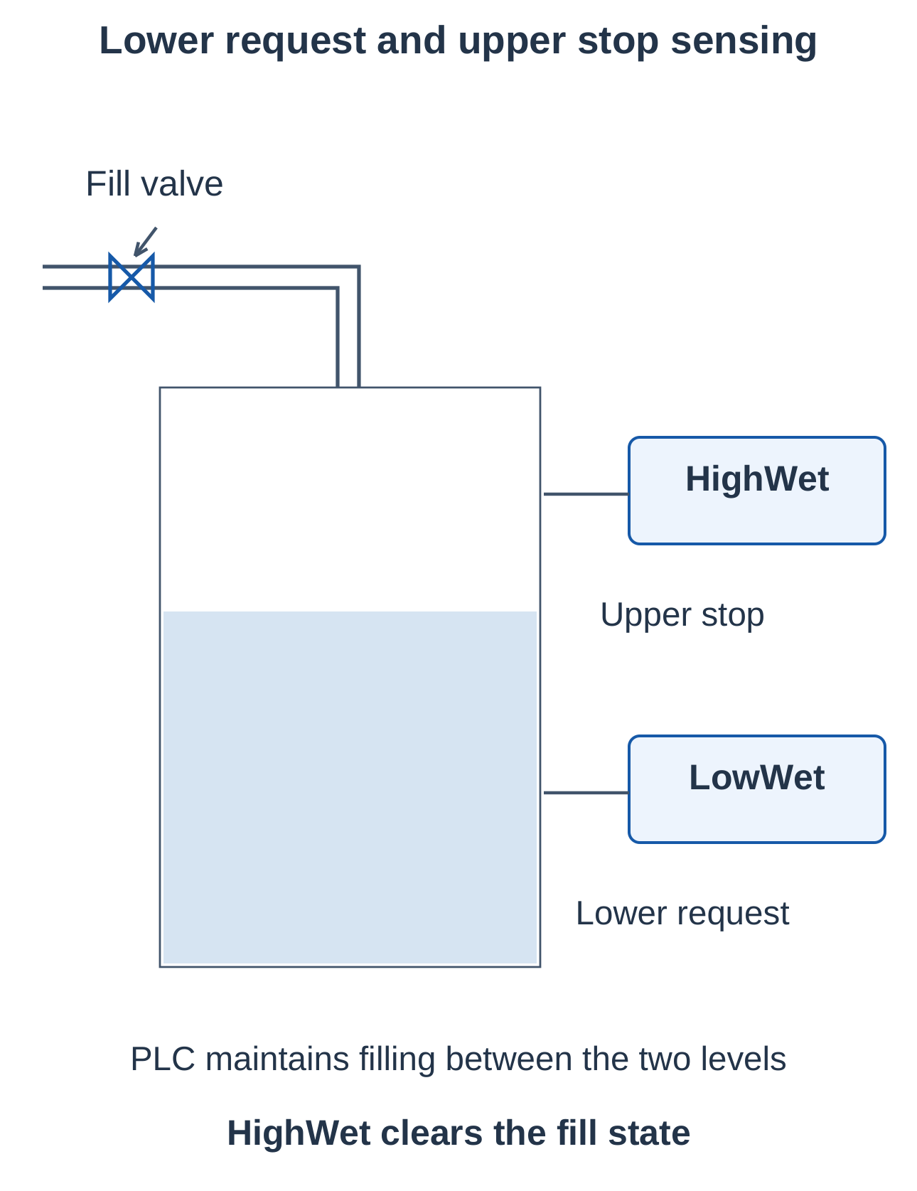
Two-Point Filling Control
Define:
- LowWet = 1: Lower sensor covered.
- HighWet = 1: Upper sensor covered.
- FillPrevious: Previously maintained filling state.
FillNext = Enable AND NOT HighWet AND (NOT LowWet OR FillPrevious)
When the lower point is uncovered, filling starts. Covering the lower point does not immediately stop it because the stored filling state maintains the command. Covering the upper point clears the command.
Add separately required equipment and fault permissions.
A metal wall generally shields the external electric field. Ordinary external capacitive sensing cannot simply detect through it. Deposits near the sensing face can also keep an output active after the main contents fall.
4.11 Comparing Sensing Principles
Inductive and Capacitive Sensors
| Feature | Inductive | Capacitive |
|---|---|---|
| Physical effect | Metal loads an alternating magnetic field | Material changes effective capacitance |
| Typical targets | Suitable metallic objects | Suitable metals, non-metals, liquids and powders |
| Main use | Metal position or tooth detection | Material presence or point-level detection |
| Important surroundings | Nearby metal and adjacent fields | Moisture, deposits and nearby materials |
| Non-metallic wall | May permit detection of a metal target | May permit detection of suitable contents |
Optical and Inductive Sensors
| Feature | Optical | Inductive |
|---|---|---|
| Sensing path | Emitted and received light | Near-field electromagnetic interaction |
| Target requirement | Suitable interruption or reflection | Suitable metal target |
| Distance capability | Can support longer paths | Usually proximity range |
| Main installation issue | Alignment and received-light margin | Gap and mounting-metal effects |
| Contamination concern | Dirty lens or obscured beam | Metal debris and changed surroundings |
Selection by Task
| Task | Suitable starting choice |
|---|---|
| Opaque carton on a conveyor | Through-beam or suitable retroreflective sensor |
| Steel mechanism position | Inductive proximity sensor |
| Liquid at one height behind a suitable plastic wall | Capacitive point-level sensor |
| Variable pressure for control | Pressure transmitter with compatible analog output |
Verify speed, repeatability, access, cleaning, mounting and signal compatibility. A suitable principle with incorrect PLC wiring still produces an unusable installation.
4.12 PNP and NPN Sensor Outputs
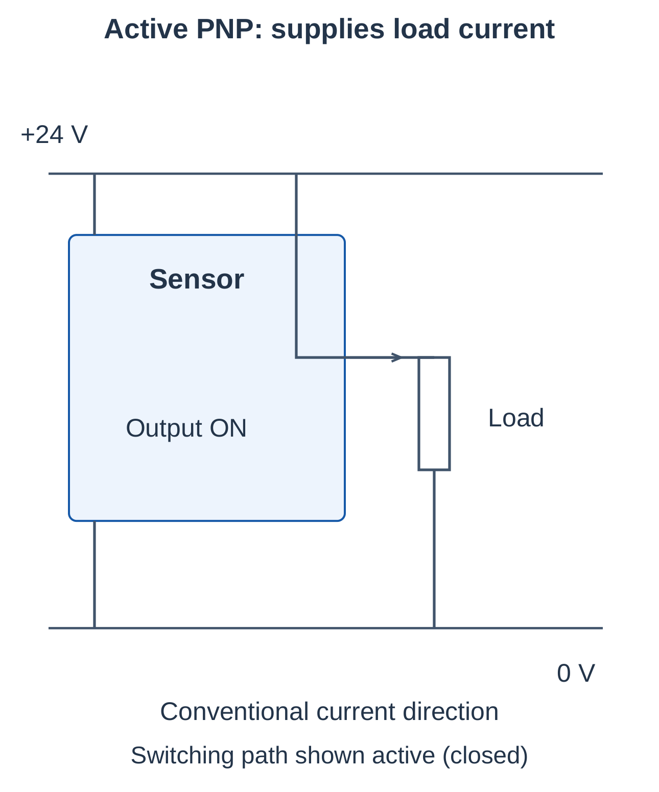
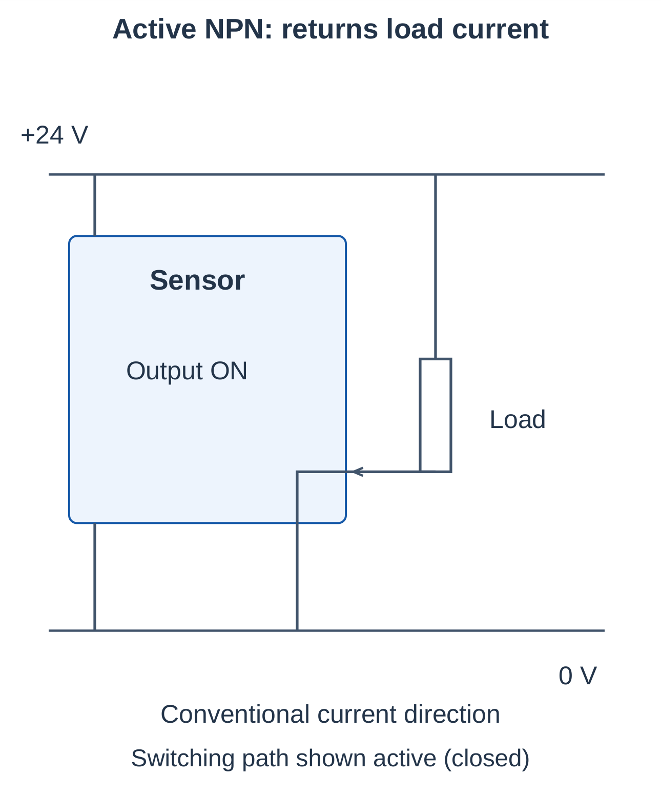
Many three-wire DC sensors contain an electronic output switch. PNP normally sources current, while NPN normally sinks current when active.
Three-Wire Connections
| Connection | Role | Common colour convention |
|---|---|---|
| Supply positive | Powers electronics | Brown |
| Supply negative | Power return | Blue |
| Switched output | Signal to input or load | Black |
Verify the device diagram. Colours and connector pin functions are not universal assumptions.
PNP Output
An active PNP output supplies current from the positive side through the load or PLC input. The connected circuit needs a suitable return to 0 V.
NPN Output
An active NPN output returns load current toward 0 V. Current passes from the positive supply through the load and into the sensor’s return switch.
PNP/NPN and NO/NC Are Separate
| Question | PNP / NPN | NO / NC |
|---|---|---|
| What does it describe? | Electrical switching arrangement | Output state relative to the defined normal sensing condition |
| Available combinations | PNP NO, PNP NC, NPN NO or NPN NC may exist | Select the required absent/present behaviour |
For an illustrative NO presence output, target absent means inactive and target present means active. An NC presence output reverses those states.
4.13 Interfacing Digital Sensors with a PLC
Match Source to Sink
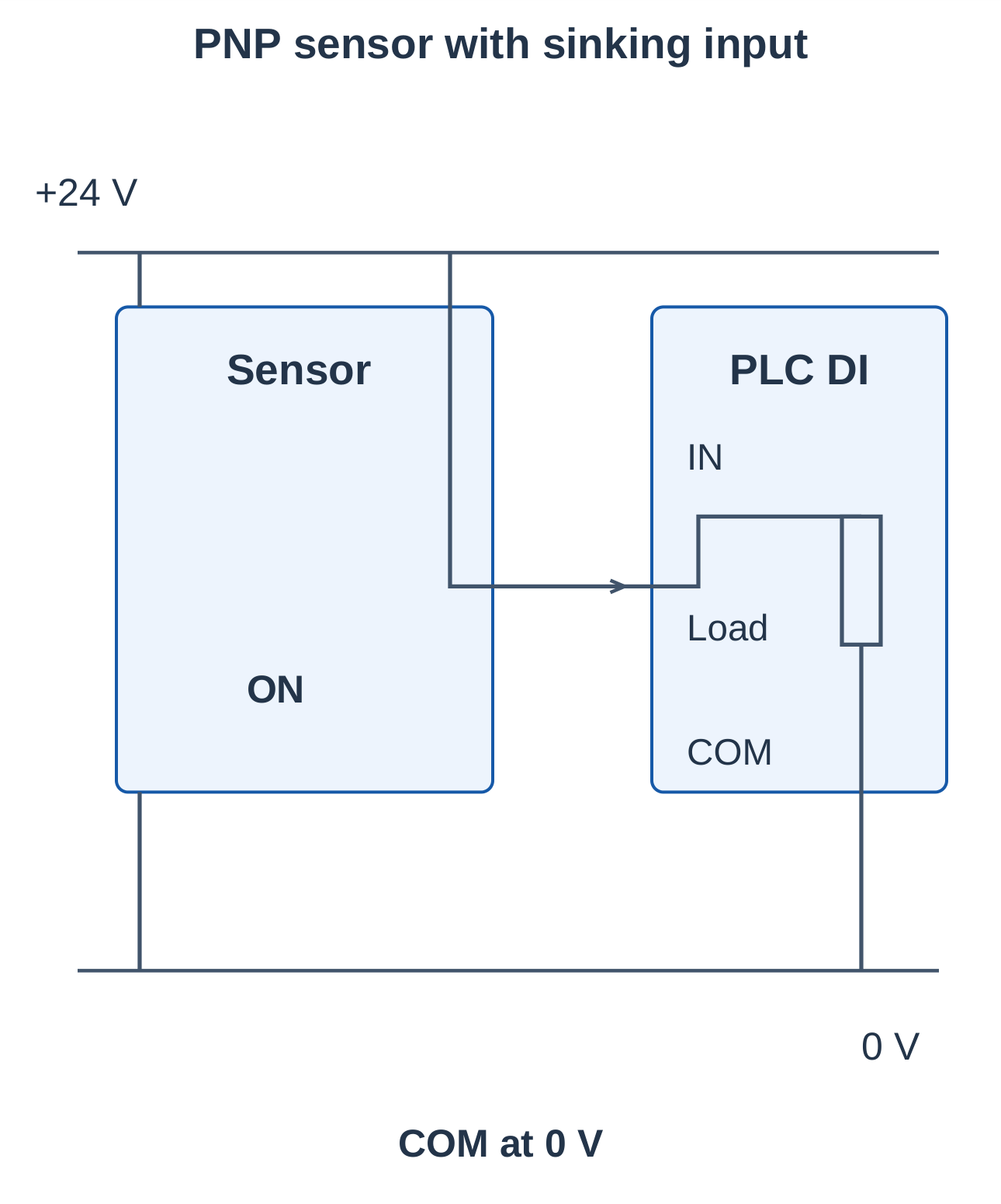
A typical PNP sensor connects to a sinking input. The sensor provides current and the input completes its return.
A typical NPN sensor connects to a sourcing input. The input supplies current and the sensor returns it.
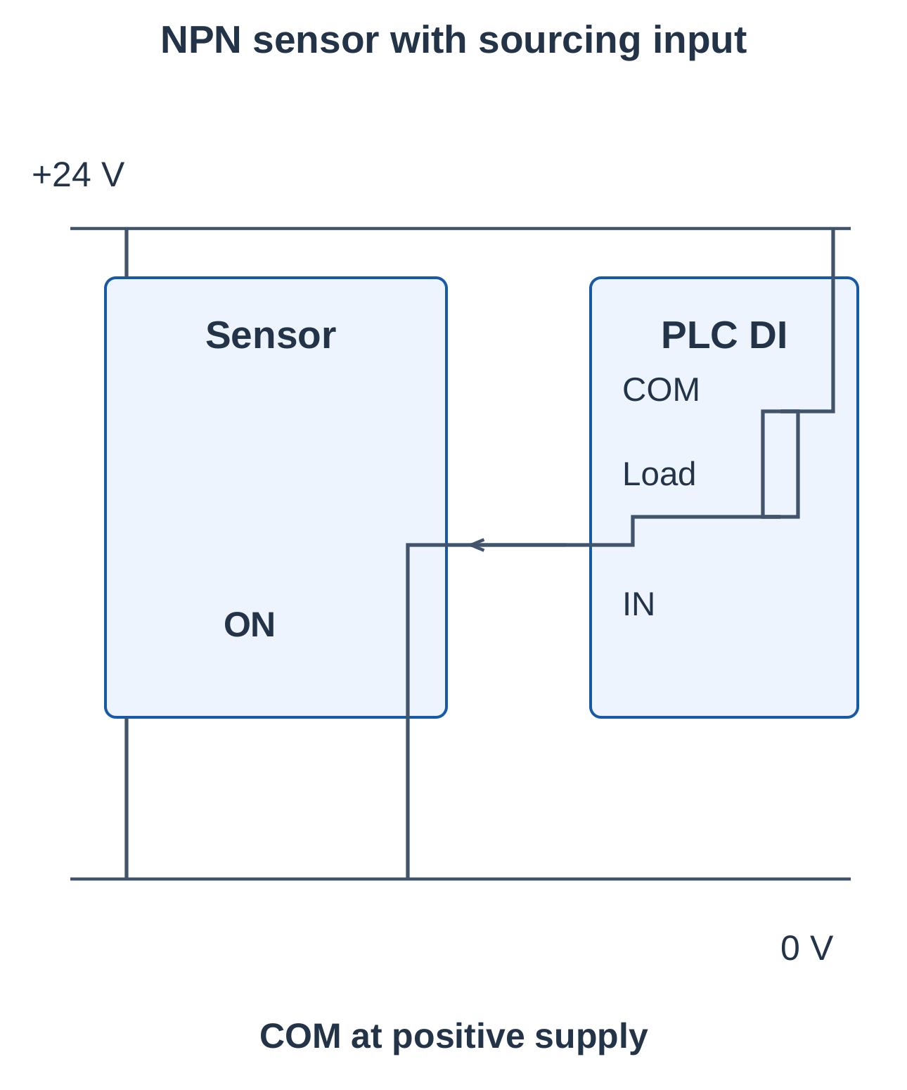
| Feature | PNP installation | NPN installation |
|---|---|---|
| Sensor role | Sources current | Sinks current |
| Matching input | Sinking | Sourcing |
| Illustrated COM | 0 V | Positive supply |
| Active current path | Supply, sensor, input, return | Supply, input, sensor, return |
Interface Checks
- Supply range and polarity.
- Active voltage and current.
- OFF-state leakage and switching drop.
- Input threshold and common reference.
- Isolation and grouped-common rules.
Some inputs share a common terminal. Do not assume that individual points can use conflicting polarity arrangements independently.
A sensor LED being ON does not prove that the PLC receives a valid input. Sensor outputs normally serve inputs or suitably rated small loads, not large motors directly. The machine needs the appropriate rated output interface, contactor or drive.
4.14 Sensor Interpretation and PLC Programming
Define the TRUE meaning of each input before writing the ladder logic.
| Tag | Meaning when TRUE |
|---|---|
| PartPresent | Configured sensor reports a part |
| PositionOK | Target at the required position |
| HighWet | Material covers the upper sensing point |
| SensorHealthy | Available diagnostic confirms the required healthy condition |
Example Permission Logic
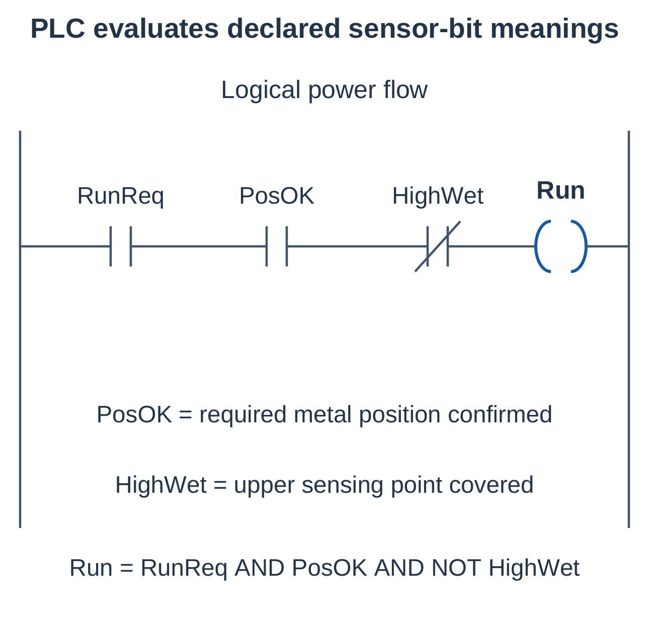
Run = RunRequest AND PositionOK AND NOT HighWet
The program tests stored bits. Electrical output polarity and physical sensing behaviour establish those bits.
One Count per Object
Pulse = PartPresent AND NOT PreviousPartPresent
Evaluate Pulse, use it to count and then update the previous-state memory. Define startup handling for an object already present, so it is not automatically mistaken for a new arrival.
Input filters can remove disturbances and short valid pulses alike. Where ordinary sampling is insufficient, use suitable high-speed input or capture facilities.
Commissioning Steps
- Verify supply and common.
- Observe the sensor output with actual target states.
- Confirm the input indication and stored bit.
- Test the program’s interpretation.
- Test motion, reset, signal loss and restoration.
An inactive input may mean either no target or a disconnected cable. Use suitable supervision where these states must be distinguished.
4.15 The 4–20 mA Current Loop
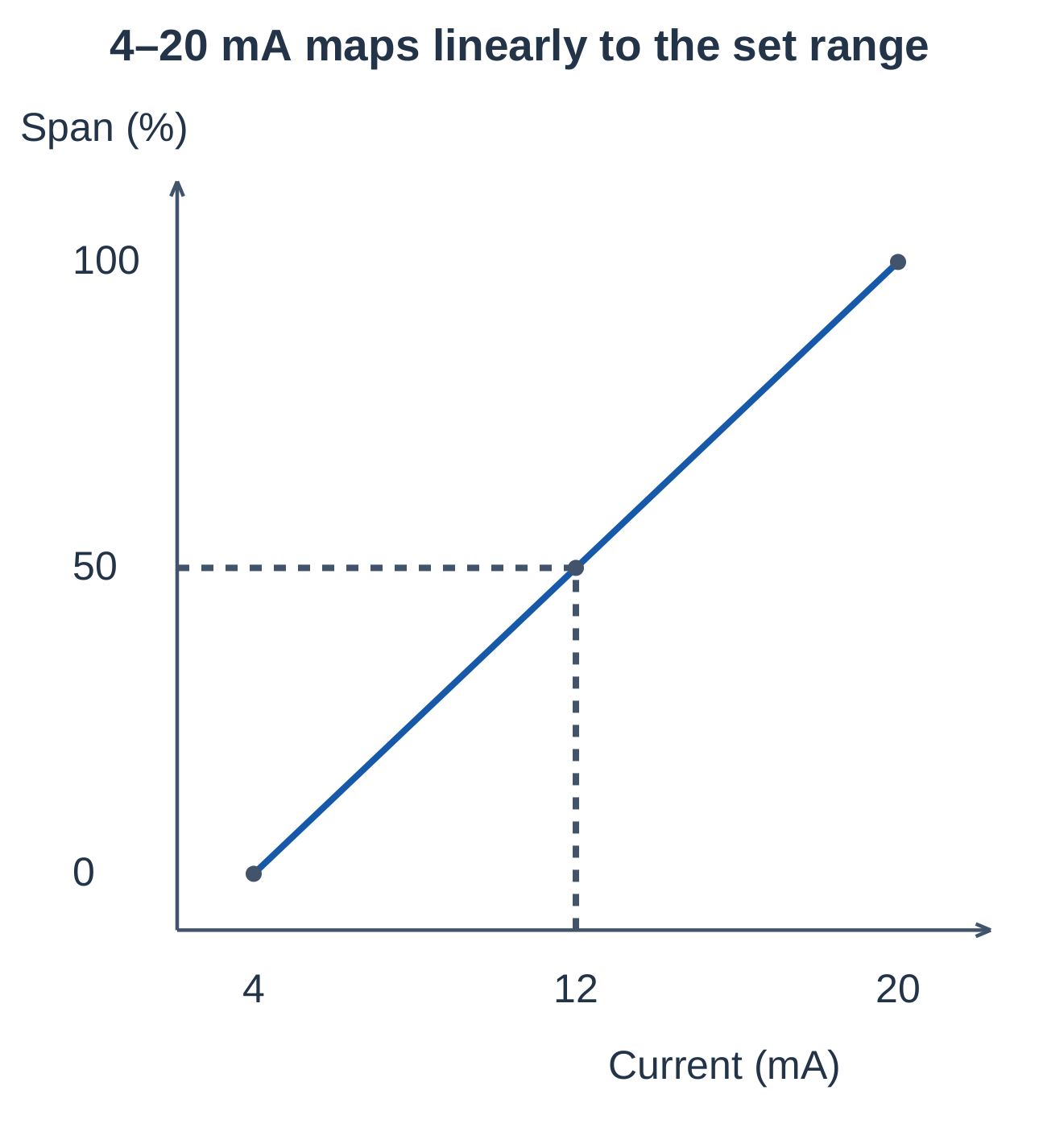
A 4–20 mA loop communicates a variable measurement or command as controlled current. For a linear measurement, 4 mA represents the lower range value and 20 mA represents the upper range value.
Basic Elements
- DC power source.
- Transmitter.
- Receiver, such as a PLC current-input module.
- Complete current return path.
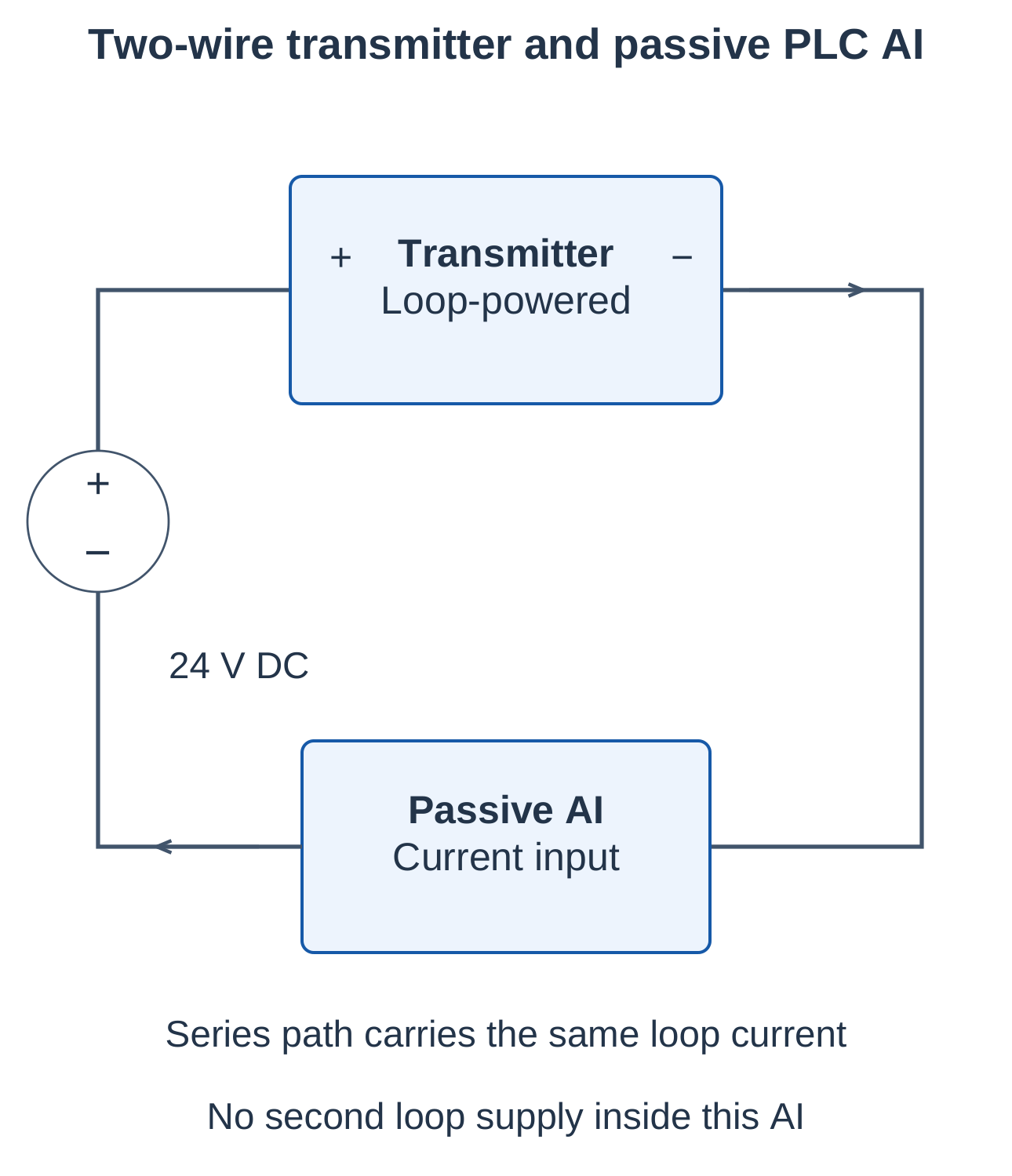
A two-wire transmitter obtains power from the same loop carrying its signal.
Live Zero
The 4 mA lower-end signal is called a live zero. It supports loop-powered transmitter operation and helps distinguish the lowest valid measurement from loss of current.
0 mA is not a normal 0% measurement on a configured 4–20 mA range. It suggests a supply, wiring or device problem. Diagnostic bands and failure direction depend on the instrument configuration.
Benefits and Limits
Within the permitted voltage and load limits, series loop elements carry the same current. Cable resistance creates voltage drop rather than directly dividing the measurement as in a simple voltage-divider circuit.
This does not allow unlimited cable resistance or remove every noise problem. Excess drop can prevent the transmitter from maintaining its current. Suitable wiring, grounding and isolation remain necessary.
An ordinary analog input reads current; it does not automatically decode HART communication.
4.16 Current-Loop Interfacing with a PLC
Active and Passive Inputs
An active current input commonly supplies loop power. A passive current input receives current and requires a suitable external powered arrangement. Confirm the manufacturer’s terminal definitions.
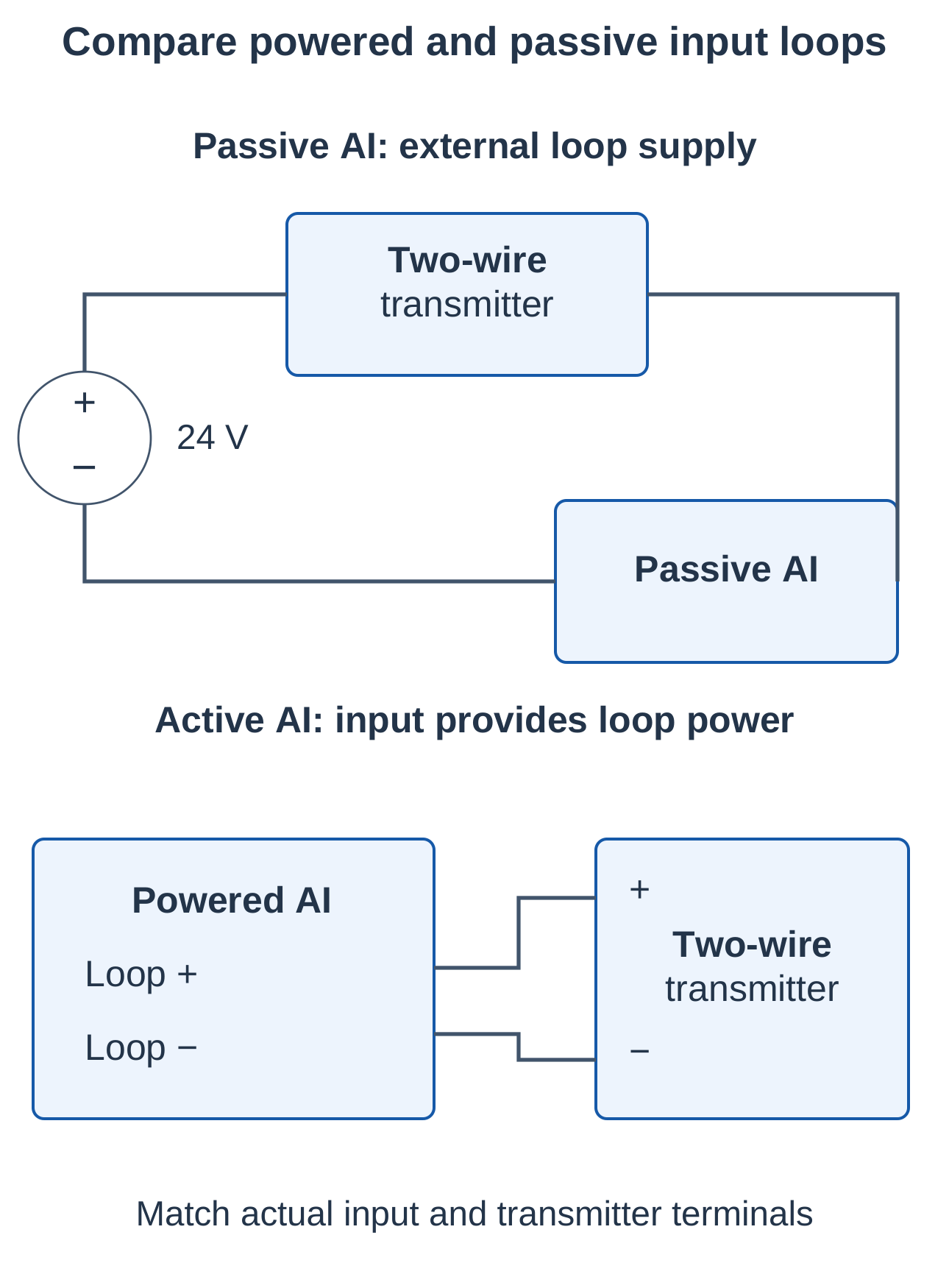
| Feature | Loop-powered two-wire transmitter | Separately powered transmitter |
|---|---|---|
| Operating power | Taken from signal loop | Separate power connections |
| Signal wiring | Same pair carries power and current | Depends on three-wire/four-wire design |
| Matching requirement | Compatible powered loop | Match sourcing output or external excitation requirements |
| Main error | Missing loop power | Conflicting supplies or incompatible interface |
Receiver Burden
A suitable resistor converts current into voltage:
V = I × R
For R = 250 Ω:
| Current | Voltage |
|---|---|
| 4 mA | 1 V |
| 12 mA | 3 V |
| 20 mA | 5 V |
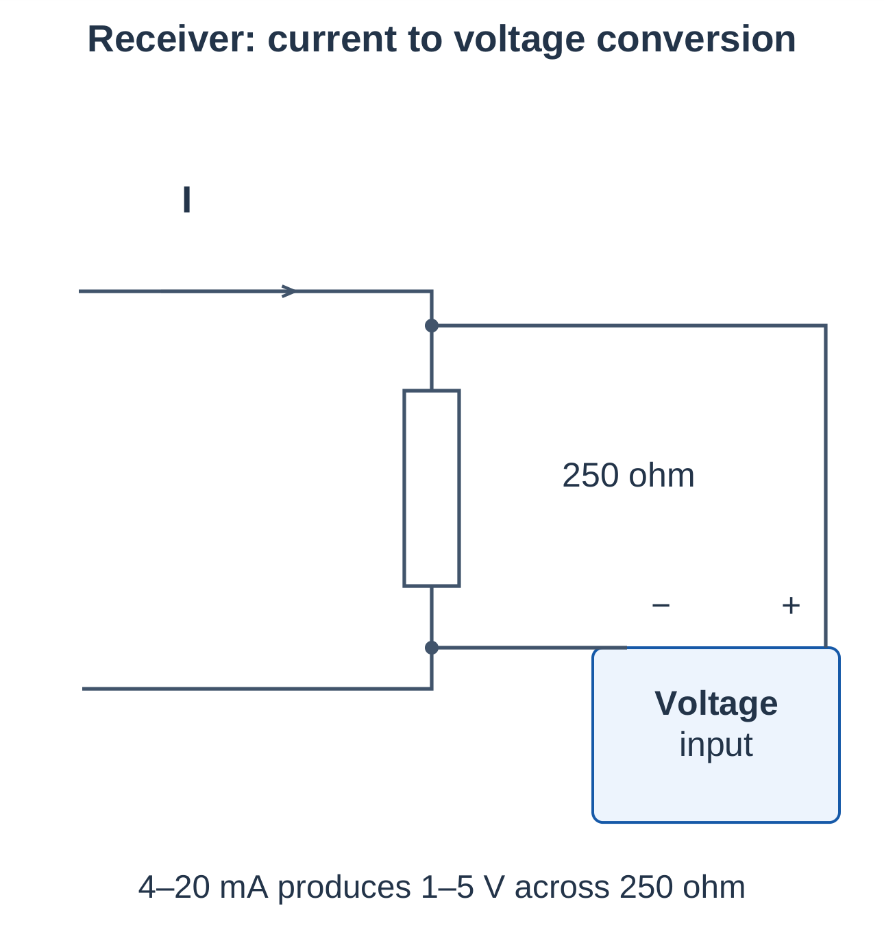
A current-input module may already contain its own sense element. Adding another resistor can create excessive burden or an incorrect connection. A voltage receiver needs the correct range, precision resistance and reference or isolation.
Resistor Dissipation Example
At 20 mA through 250 Ω:
P = I²R = (0.020)² × 250 = 0.10 W
This is nominal dissipation. Select an actual rating with appropriate margin, temperature and tolerance considerations.
4.17 Scaling, Span and Worked Examples
Let LRV be the lower range value, URV the upper range value and I the current in mA.
Fraction of span = (I − 4) / 16
Measurement = LRV + [(I − 4) / 16] × (URV − LRV)
For the inverse conversion:
I = 4 + 16 × (Measurement − LRV) / (URV − LRV)
Pressure Example
For a 0–10 bar transmitter at 12 mA:
Fraction = (12 − 4) / 16 = 0.5
Pressure = 0 + 0.5 × 10 = 5 bar
At 16 mA:
Pressure = [(16 − 4) / 16] × 10 = 7.5 bar
Nonzero Lower Range Example
Temperature range = −20 to 80°C; current = 8 mA:
Fraction = (8 − 4) / 16 = 0.25
Temperature = −20 + 0.25 × 100 = 5°C
Map 4 mA to the actual lower range value, which is not necessarily zero.
Raw-Count Scaling
If Raw4 and Raw20 are the configured counts at 4 and 20 mA:
Measurement = LRV + [(Raw − Raw4) / (Raw20 − Raw4)] × (URV − LRV)
Use the module’s documented convention. A 4–20 mA range and a 0–20 mA range may use different raw representations.
Validate signal quality before using the result. Define responses to invalid current, stale data and device faults. Silently treating every fault as 0% can hide a failed measurement.
4.18 Loop Voltage Budget and Fault Tracing
Compliance Voltage
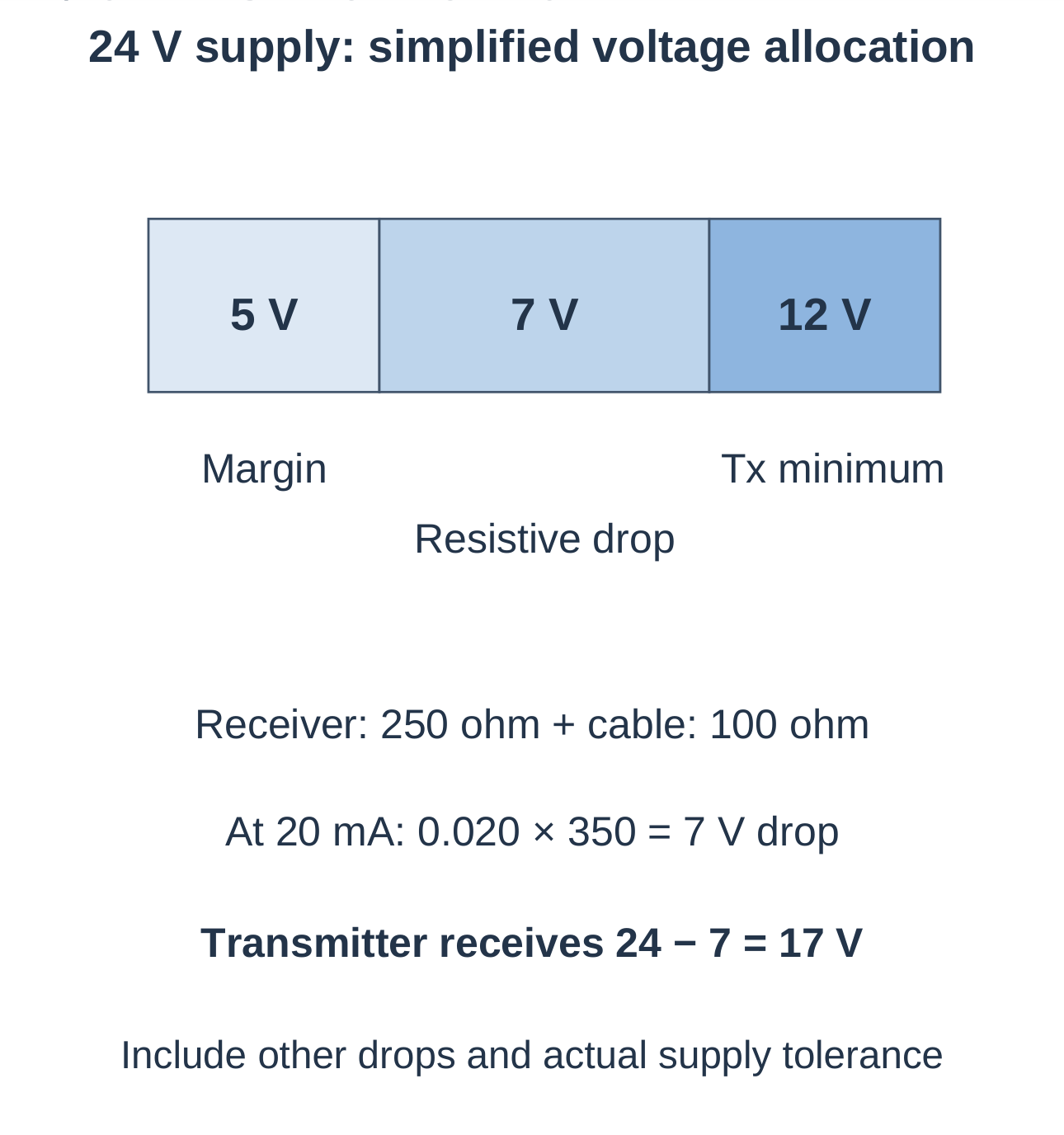
The supply must cover the transmitter’s minimum terminal voltage, resistive drops and other series drops.
Vs ≥ Vt + Imax × RL + Vd
RL,max = (Vs − Vt − Vd) / Imax
| Symbol | Meaning |
|---|---|
| Vs | Supply voltage |
| Vt | Minimum transmitter operating voltage |
| Imax | Required maximum loop current |
| RL | Total series resistance |
| Vd | Other series voltage drops |
Worked Voltage Budget
Given:
- Supply = 24 V.
- Minimum transmitter voltage = 12 V.
- Receiver resistance = 250 Ω.
- Total cable resistance = 100 Ω.
- Maximum current = 20 mA.
- No other specified series drop.
Resistive drop = 0.020 × (250 + 100) = 7 V
Transmitter voltage = 24 − 7 = 17 V
Margin above minimum = 17 − 12 = 5 V
Maximum total resistance = (24 − 12) / 0.020 = 600 Ω
After allocating 250 Ω to the receiver:
Remaining simplified resistance allowance = 600 − 250 = 350 Ω
Account for actual supply tolerance, other drops and design margin in a real selection.
Loop Fault Diagnosis
| Observation | Checks |
|---|---|
| Zero or nearly zero current | Supply, open circuit, polarity and device failure |
| Current cannot reach the upper end | Burden, cable drop, supply and transmitter condition |
| Correct current but wrong PLC value | Channel range, scaling and units |
| Erratic reading | Connections, grounding, shielding, noise and real process variation |
| Diagnostic out-of-range current | Device status and alarm configuration |
An ammeter is inserted in series; a voltage measurement is taken across the intended element. Do not place a low-resistance current-measuring connection across the supply.
4.19 HART Protocol Fundamentals
HART stands for Highway Addressable Remote Transducer. Conventional wired HART combines a 4–20 mA analog process signal with bidirectional digital communication on the same pair.
The analog path carries a configured primary measurement. Digital communication can provide measurements, units, identification, configuration and diagnostic information through supported commands.
Classic Wired HART Signalling
Classic wired HART uses frequency-shift keying, or FSK.
| Parameter | Value in the classic wired model |
|---|---|
| Digital 1 tone | 1200 Hz |
| Digital 0 tone | 2200 Hz |
| Bit rate | 1200 bit/s |
| Nominal digital current component | Approximately ±0.5 mA around the analog level |
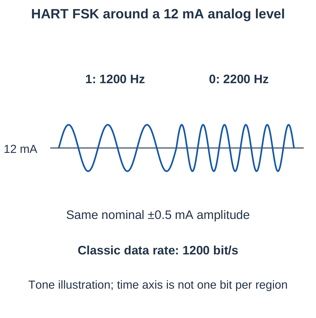
The alternating component has essentially zero average. A suitable analog input can recover the underlying current, while a compatible modem decodes the digital messages.
Tone frequency and bit rate are different. The 2200 Hz tone is not another data rate.
Analog and Digital Paths
| Analog path | Digital path |
|---|---|
| One configured process value represented by current | Identified values, units, status and supported information |
| Read by a suitable ordinary analog input | Requires a HART-compatible interface or communicator |
| Interpretation depends on configured LRV and URV | Access depends on commands and device support |
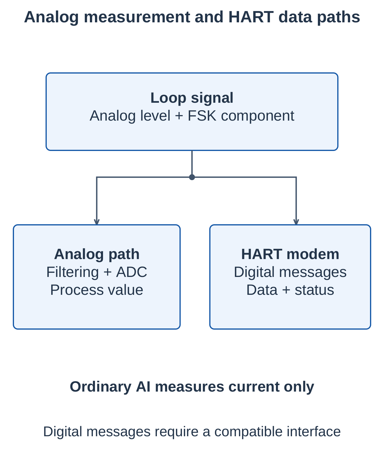
A HART transmitter does not automatically turn an ordinary PLC analog input into a HART modem.
4.20 HART Point-to-Point Configuration
A point-to-point loop contains one intended field device connected to the host interface. Its analog current can track the process variable while digital messages supply additional information.
Primary and Secondary Hosts
The control-system interface commonly serves as the primary host. A compatible handheld communicator can serve as a secondary host. Host coordination must prevent conflicting operations or configuration changes.
Loop Impedance and Communicator Access
HART needs suitable loop impedance to develop a detectable digital signal. A 250 Ω burden is common, but equipment specifies the actual resistance and capacitance limits.
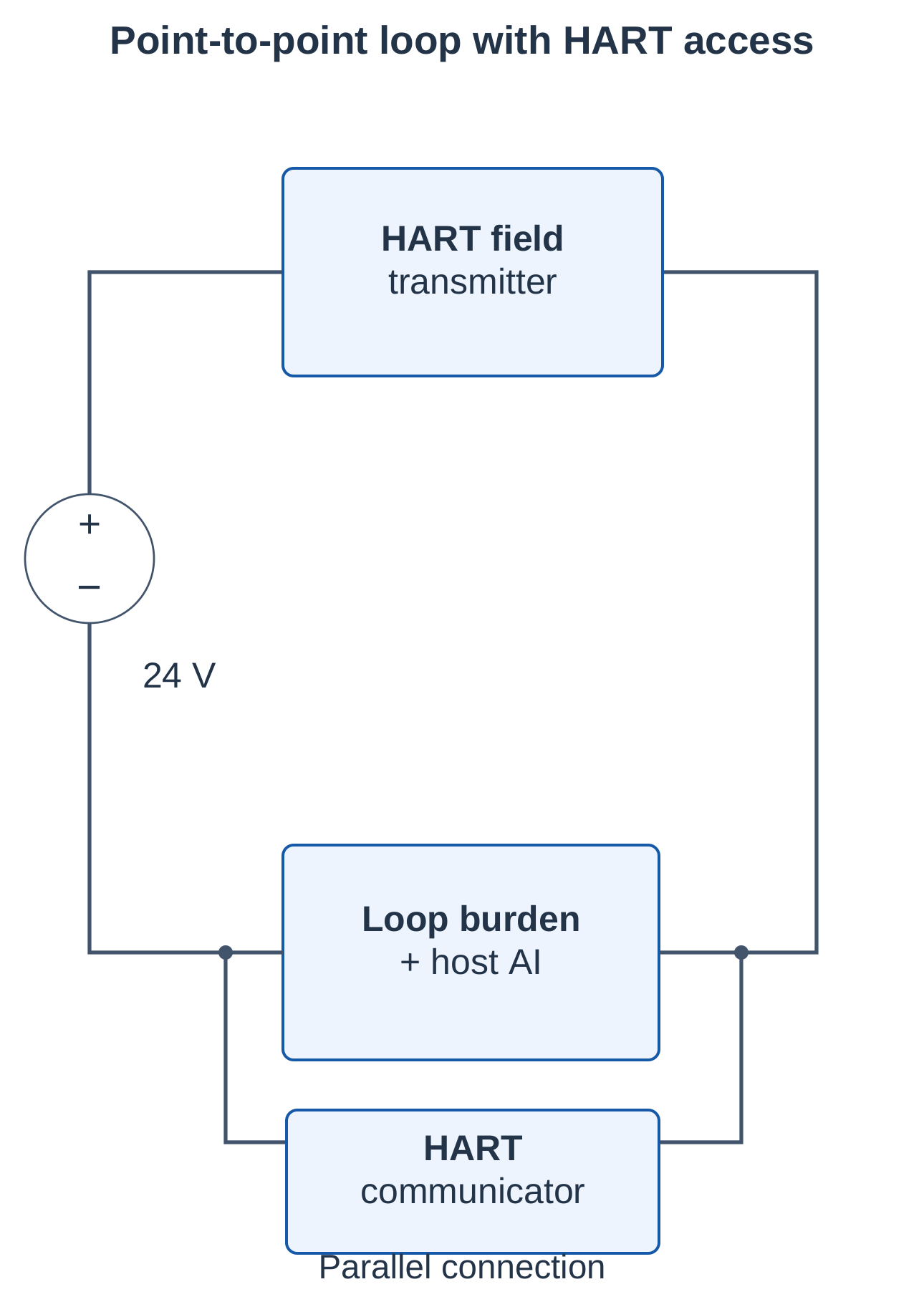
The input may already provide sufficient burden. Do not automatically add another resistor. Any barrier, isolator or conditioner in the path must pass HART signalling where communication is required.
A communicator normally connects in parallel according to its instructions, rather than as a series ammeter.
Typical Uses
- Read device identity and measurement units.
- Examine status and diagnostics.
- Configure the measurement range.
- Perform a supported fixed-current loop test.
- Compare analog interpretation with the digital measurement.
Changing the transmitter range changes what its current represents. Update PLC scaling accordingly.
4.21 HART Multidrop Configuration
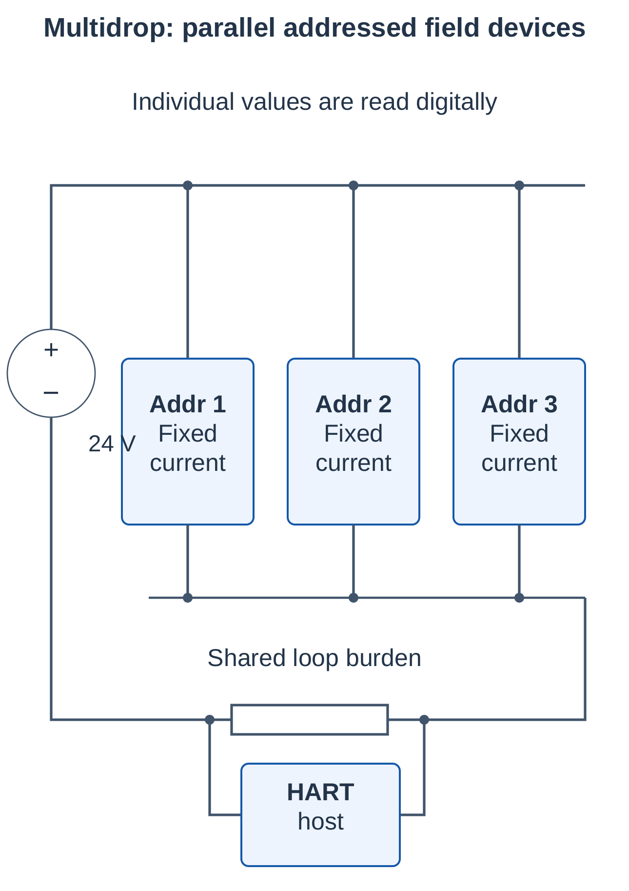
A conventional multidrop arrangement connects multiple compatible addressed devices to a shared communication pair. Individual measurements are obtained digitally.
Fixed-Current Operation
In the usual multidrop configuration, loop-current process tracking is disabled and each device draws a configured fixed current, commonly 4 mA.
Four devices drawing 4 mA each require approximately:
Total device current = 4 × 4 = 16 mA
This combined current is not an independent analog measurement for each device.
Addressing and Revision
- Older HART 5 multidrop installations commonly use addresses 1–15.
- HART revision 6 and later support polling addresses 0–63.
- Actual supported device count depends on the host and electrical limits.
- Later implementations may configure loop-current mode separately from the address.
Do not assume that changing the address alone changes analog-output behaviour on every device. Configure unique addresses and current mode according to the equipment instructions.
Point-to-Point and Multidrop Comparison
| Feature | Point-to-point | Conventional multidrop |
|---|---|---|
| Field devices | One per illustrated loop | Several addressed devices |
| Process measurement | Analog current plus digital data | Individual values obtained digitally |
| Typical current behaviour | Tracks configured variable | Fixed current per device, commonly 4 mA |
| Identification | One intended field device | Unique addresses essential |
| Update consideration | One device and host traffic | Shared polling and message traffic |
| Application | Analog process loop with diagnostics | Several digitally monitored devices on one pair |
4.22 HART Communication Modes
Point-to-point/multidrop describe configuration. Request–response/burst describe message behaviour. These are separate distinctions.
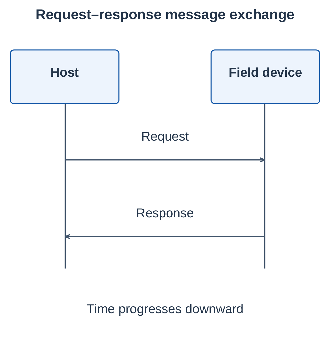
Request–Response
Classic wired HART uses half-duplex communication: one direction transmits at a time on the shared channel.
- The host sends a command to an addressed device.
- The device returns the defined response.
- The response can contain measurements or supported status and configuration information.
Burst Operation
A compatible device can be configured to repeatedly transmit a selected supported message under burst rules. This reduces the need for a new request before every repeated update.
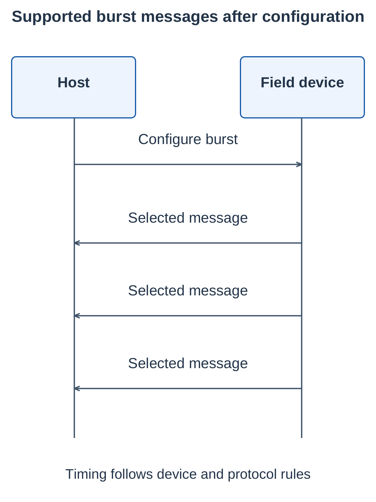
Burst support, scheduling and coexistence depend on device and host capabilities. Burst is not a separate voltage signal and does not provide unlimited update speed; the classic 1200 bit/s channel still limits throughput.
Mode Comparison
| Feature | Request–response | Burst |
|---|---|---|
| Trigger | Host command | Configured device transmission behaviour |
| Pattern | Request followed by response | Repeated selected messages |
| Purpose | Specific reads and configuration | Repeated information updates |
| Requirement | Supported host and device commands | Burst-capable device and compatible host handling |
Command Groups
- Universal commands: Common supported information.
- Common-practice commands: Broadly used functions with device-dependent support.
- Device-specific commands: Functions particular to a device family.
For an examination answer, explain who initiates the message, what information it carries and how the mode differs from the network configuration.
4.23 Integrated Applications and Commissioning
Packaging-Station Example
Different tasks can require different sensing principles:
| Task | Sensor |
|---|---|
| Carton arrival | Optical sensor |
| Metal mechanism position | Inductive sensor |
| Material at a defined height | Capacitive sensor |
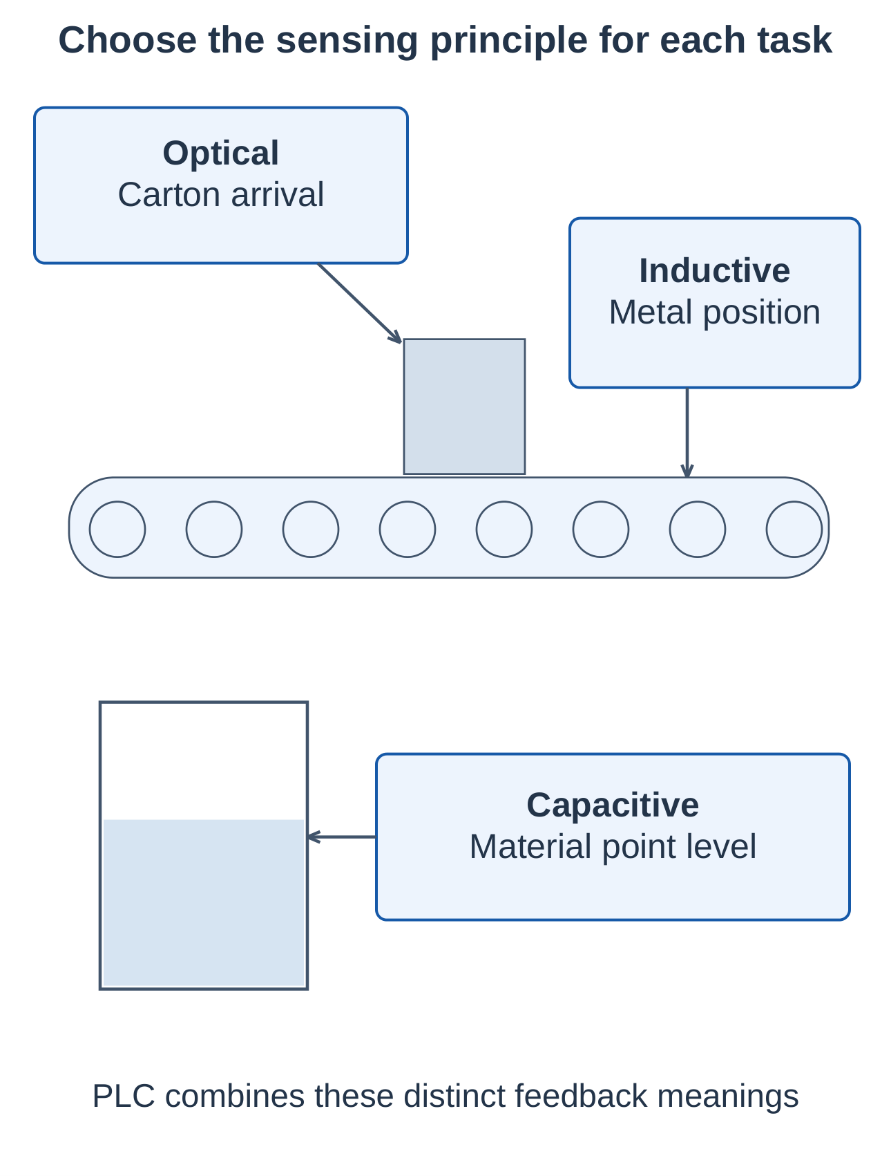
The PLC assigns explicit bit meanings, evaluates permissions and commands rated equipment interfaces.
Pressure-Loop Example
A transmitter has a 0–10 bar range and a 4–20 mA output. At 12 mA, the expected PLC value is 5 bar. A HART-capable tool can separately inspect the digital measurement, configured range and device status.
If analog interpretation is wrong, distinguish transmitter configuration from PLC scaling and loop electrical faults. Disagreement can involve range settings, sensor trim, output trim or acquisition error. Investigate before changing calibration.
Commissioning Procedure
- Inspect installation and the actual target or process.
- Verify supply, polarity, common and interface type.
- Test digital states or analog endpoints.
- Confirm PLC tags and engineering units.
- Verify communication and address settings where used.
- Test fault response and recovery.
HART Fault Checks
| Observation | Checks |
|---|---|
| Analog signal works but no HART response | Compatible interface, impedance, address and signal-transparent path |
| Only one multidrop device found | Unique addresses, polling range, supply and branch wiring |
| Intermittent communication | Connections, interference, capacitance and conditioning compatibility |
| Digital value differs from analog value | Range, scaling, current mode, fixed-current test and trim |
| Process current unexpectedly fixed | Multidrop/current-mode settings or active loop test |
One normal LED or plausible current value does not verify the whole system. Test the path from physical condition through sensor, wiring, input and program to the controlled response.
4.24 Quick Revision and Examination Practice
Essential Revision Points
- Optical sensors evaluate received light.
- Through-beam uses separate emitter and receiver housings.
- Retroreflective sensing uses a separate reflector.
- Diffuse sensing uses light returned by the target.
- Inductive sensors detect suitable metals through alternating-field interaction.
- Capacitive sensors detect material-induced capacitance changes.
- PNP outputs normally match sinking inputs; NPN outputs normally match sourcing inputs.
- NO/NC behaviour is separate from PNP/NPN wiring.
- A 4–20 mA loop uses live zero and needs sufficient voltage for every series drop.
- Current, raw count and engineering value are different representations.
- Classic wired HART adds FSK communication to the analog loop.
- Network configuration and communication mode must be distinguished.
Important Formulas
| Formula | Application |
|---|---|
| Hysteresis = Release distance − Operate distance | Illustrated proximity-switch model |
| Event rate = Features × rpm / 60 | Rotating-target detection |
| C = ε₀ εᵣ A / d | Ideal parallel-plate capacitance |
| Fraction = (I − 4) / 16 | Current-loop fraction, I in mA |
| Value = LRV + Fraction × (URV − LRV) | Engineering scaling |
| V = IR | Burden voltage |
| P = I²R | Resistor dissipation |
| RL,max = (Vs − Vt − Vd) / Imax | Simplified loop resistance limit |
Numerical Practice with Answers
| Problem | Answer |
|---|---|
| Operate at 6 mm; release at 6.6 mm | Hysteresis 0.6 mm; 10% relative to operate distance |
| Gear with 20 teeth at 180 rpm | 20 × 180 / 60 = 60 Hz |
| Pressure range 0–16 bar at 10 mA | Fraction 0.375; pressure 6 bar |
| Temperature range 20–120°C at 16 mA | 20 + 0.75 × 100 = 95°C |
| Required current for 75% of span | 4 + 16 × 0.75 = 16 mA |
| 20 mA through 250 Ω | 5 V; nominal dissipation 0.10 W |
| Supply 24 V, transmitter minimum 10 V, other drop 2 V, Imax 20 mA | Maximum total resistance 600 Ω |
| Five multidrop devices drawing 4 mA each | Approximately 20 mA total; individual measurements are digital |
Long-Answer Questions
- Draw and explain through-beam, retroreflective and diffuse sensing.
- Explain inductive construction, eddy-current operation and mounting.
- Explain capacitive detection and external point-level sensing through a suitable wall.
- Compare inductive and capacitive sensors in separate columns.
- Draw PNP/sinking-input and NPN/sourcing-input current paths.
- Explain a two-wire 4–20 mA loop, live zero and PLC scaling.
- Derive a loop voltage budget and solve a numerical example.
- Explain HART signalling and compare point-to-point with multidrop.
- Compare request–response and burst communication.
Short-Answer Questions
- Why does PNP not mean normally open?
- Why can dark and bright targets produce different diffuse-sensor responses?
- What is the purpose of sensor hysteresis?
- Why is 0 mA not a valid zero measurement on a 4–20 mA range?
- Why does an ordinary analog input not automatically read HART data?
- Why do multidrop devices need unique addresses?
Frequently Asked Questions
What does Industrial Automation and Control Unit 4 cover?
Unit 4 covers industrial sensors and their applications, including optical, inductive and capacitive detection, PNP/NPN outputs, PLC connections, current loops and HART.
What is the main difference between inductive and capacitive sensors?
Inductive sensing detects suitable metals through their effect on an alternating magnetic field. Capacitive sensing detects changes in effective capacitance and can respond to suitable metallic and non-metallic materials.
What does 4 mA represent?
It represents the configured lower range value in a linear 4–20 mA measurement. That value may be zero, a positive number or a negative number.
Can an ordinary PLC analog input read HART messages?
It can measure compatible analog current. Digital HART messages require a compatible modem, interface or communicator.
How should a sensor application be studied?
Identify the target, sensing principle, output, PLC connection and bit meaning. For an analog loop, also check range, voltage budget, scaling and quality. For HART, distinguish configuration from message mode.