
Industrial Automation and Control Unit 3 Notes explain how a programmable logic controller connects field signals with a stored control program. This unit, Automation using PLC, covers digital and analog interfaces, sinking and sourcing circuits, ladder programming, sequential function charts, timers, counters and numerical calculations.
These notes are for AKTU B.Tech 5th Semester EE and EN students studying BEE053. The explanations include labelled diagram positions, worked examples and revision questions for understanding the unit and preparing examination answers.
Topics Covered
| Topic | Topic |
|---|---|
| 3.1 PLC input and output foundation | 3.13 Off-delay timer: TOF |
| 3.2 Digital inputs and outputs | 3.14 Retentive timer |
| 3.3 Analog inputs, outputs and scaling | 3.15 Cyclic timers |
| 3.4 Sinking and sourcing concepts | 3.16 Timer selection and problems |
| 3.5 Sinking and sourcing outputs | 3.17 Counters and pulse interpretation |
| 3.6 Ladder diagram fundamentals | 3.18 Up-counter: CTU |
| 3.7 Start–stop holding logic | 3.19 Down-counter: CTD |
| 3.8 Programming practices and scan effects | 3.20 Up/down counting |
| 3.9 Sequential function chart | 3.21 Math instructions and data types |
| 3.10 Fill, hold and drain sequence | 3.22 Comparison and worked math problems |
| 3.11 Timer instruction foundation | 3.23 Integrated carton-batching example |
| 3.12 On-delay timer: TON | 3.24 Revision and examination practice |
3.1 PLC Input and Output Foundation
A PLC input supplies information about a field condition. A PLC output supplies a command to an appropriate device or interface. The electrical circuit determines how a signal reaches the controller; the program determines how the stored signal is used.
Four Basic Signal Classes
| Signal class | Information carried | Example |
|---|---|---|
| Digital input: DI | Discrete state | Pushbutton or presence sensor |
| Digital output: DO | Discrete command | Lamp or contactor interface |
| Analog input: AI | Variable measurement | Temperature or tank level |
| Analog output: AO | Variable command | Valve-position or drive-speed reference |
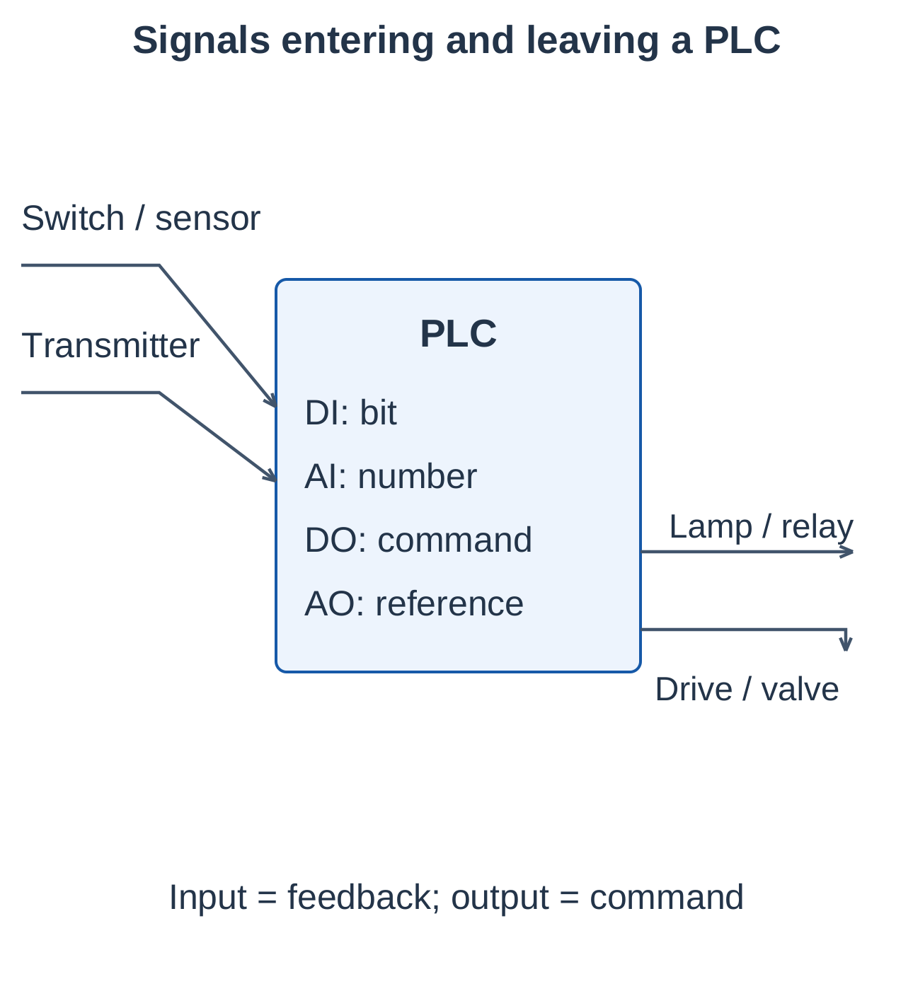
A transmitter sends its measurement toward a PLC input. An output sends a command toward a load. A networked drive can exchange both commands and status, so command information must still be distinguished from feedback.
Process Image and Physical Signals
A conventional cyclic program reads stored input information, executes its logic and updates output information. A physical input can change between scans. Consequently, a stored input bit is a sampled representation of the field signal.
Before connecting I/O, check:
- Voltage and current requirements.
- AC or DC operation and polarity.
- Common connections and isolation.
- Input filtering and permitted load duty.
Matching connectors do not establish electrical compatibility. Software cannot repair an incompatible current path.
3.2 Digital Inputs and Outputs
Digital Input Operation
A digital input classifies its electrical signal using the module’s defined thresholds. The input may receive current through a switch or a transistor sensor output. Filtering can reject brief disturbances, but it can also delay a valid change.
Physical NO/NC Contacts and Program Bits
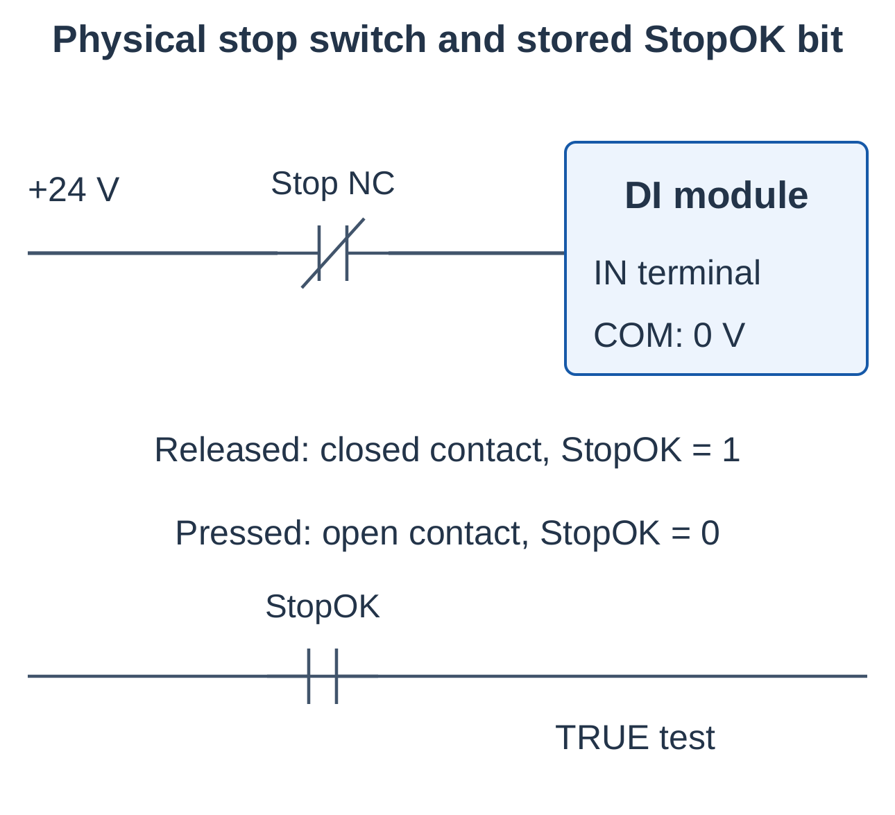
Consider a physical normally closed stop switch wired so that the input is energized while the switch is healthy and unpressed.
| Physical condition | Stop contact | StopOK input bit |
|---|---|---|
| Released and healthy | Closed | 1 |
| Pressed | Open | 0 |
The program should test StopOK for TRUE when this bit means permission to run. A ladder symbol tests stored information; its appearance does not have to match the physical contact type.
Output Technologies
| Feature | Relay output | Transistor output |
|---|---|---|
| Switching element | Mechanical contact | Semiconductor |
| Supply suitability | AC/DC within contact ratings | Specified DC arrangement |
| Switching speed | Limited by mechanical operation | Often faster within specified limits |
| Main considerations | Contact wear and condition | Leakage current and voltage drop |
A triac output generally serves suitable AC loads. Output technologies have different current, frequency, isolation and load limits.
A PLC output can operate a small lamp or coil within its rating. A motor normally requires suitable switching equipment, such as a contactor or drive. Protection and inductive suppression must match the hardware.
Pulse Detection Limit
A short sensor pulse can occur completely between ordinary input samples. High-speed counting, interrupts or suitable pulse conditioning may be required. Changing ladder logic cannot recover an event that the input system never captured.
3.3 Analog Inputs, Outputs and Scaling
Analog Input Conversion
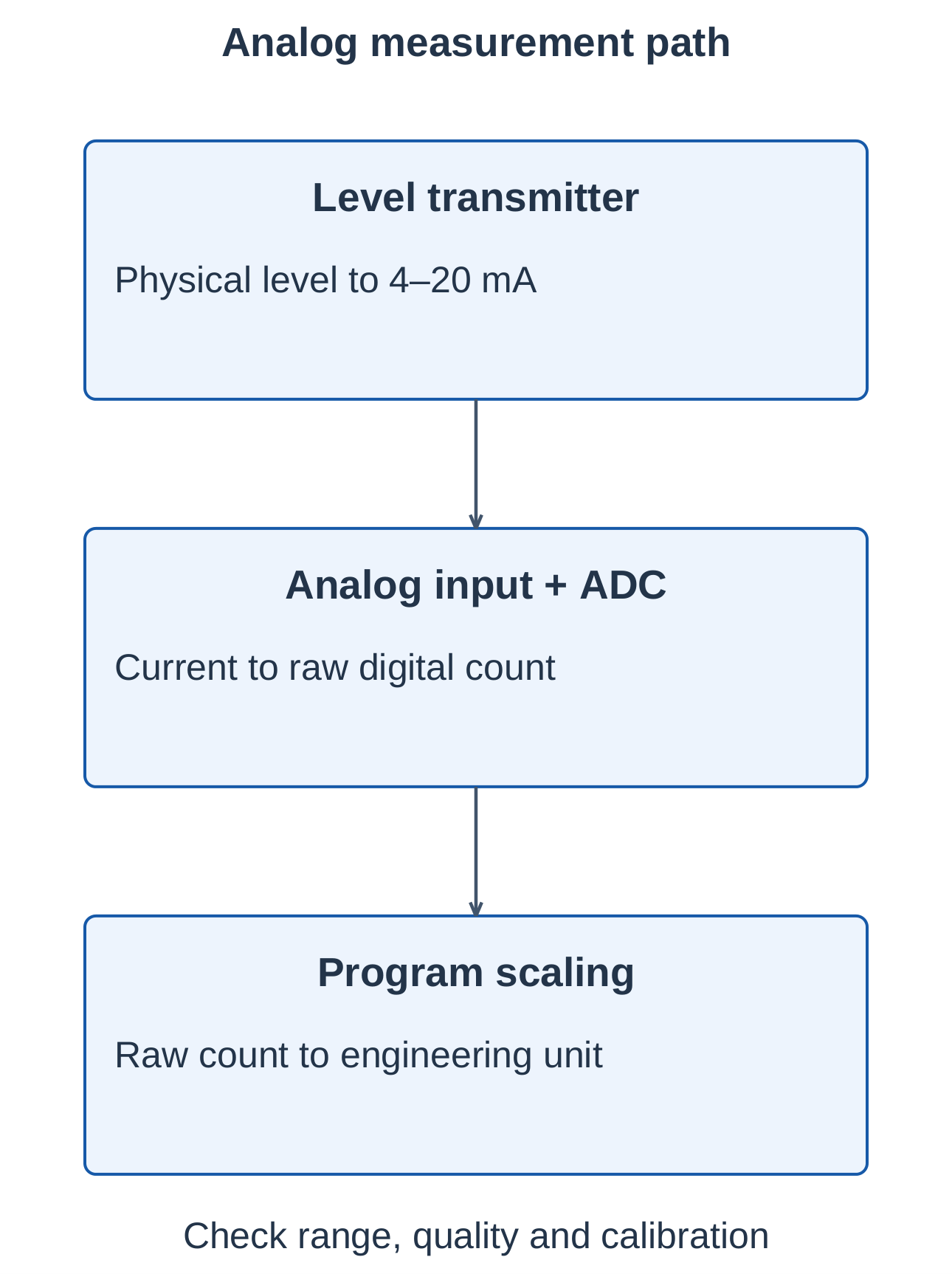
An analog input converts an electrical measurement into a numerical value using analog-to-digital conversion. The program must interpret the configured range, numerical format and diagnostic status.
Typical industrial signals include 0–10 V and 4–20 mA, subject to module support. Temperature measurement may require a dedicated sensor and conversion arrangement.
Resolution and Accuracy
Resolution describes the representable increment. Accuracy describes closeness to the true or accepted value under stated conditions. More bits do not automatically remove sensor error, calibration error or noise.
An ideal n-bit conversion has 2ⁿ codes. If codes 0 to 2ⁿ − 1 map exactly to both range endpoints:
One code interval = Measurement span / (2ⁿ − 1)
Use the module’s convention because specifications may define quantization steps differently.
Linear Scaling Formula
Engineering value = E_min + (Raw − R_min) × (E_max − E_min) / (R_max − R_min)
| Symbol | Meaning |
|---|---|
| Raw | Measured numerical input |
| R_min, R_max | Configured raw endpoints |
| E_min, E_max | Corresponding engineering endpoints |
Do not assume that every PLC uses the same raw count range.
Worked Scaling Examples
Example 1: Raw counts to tank level
Raw 0–4000 represents level 0–100%. At Raw = 2600:
Level = (2600 / 4000) × 100 = 65%
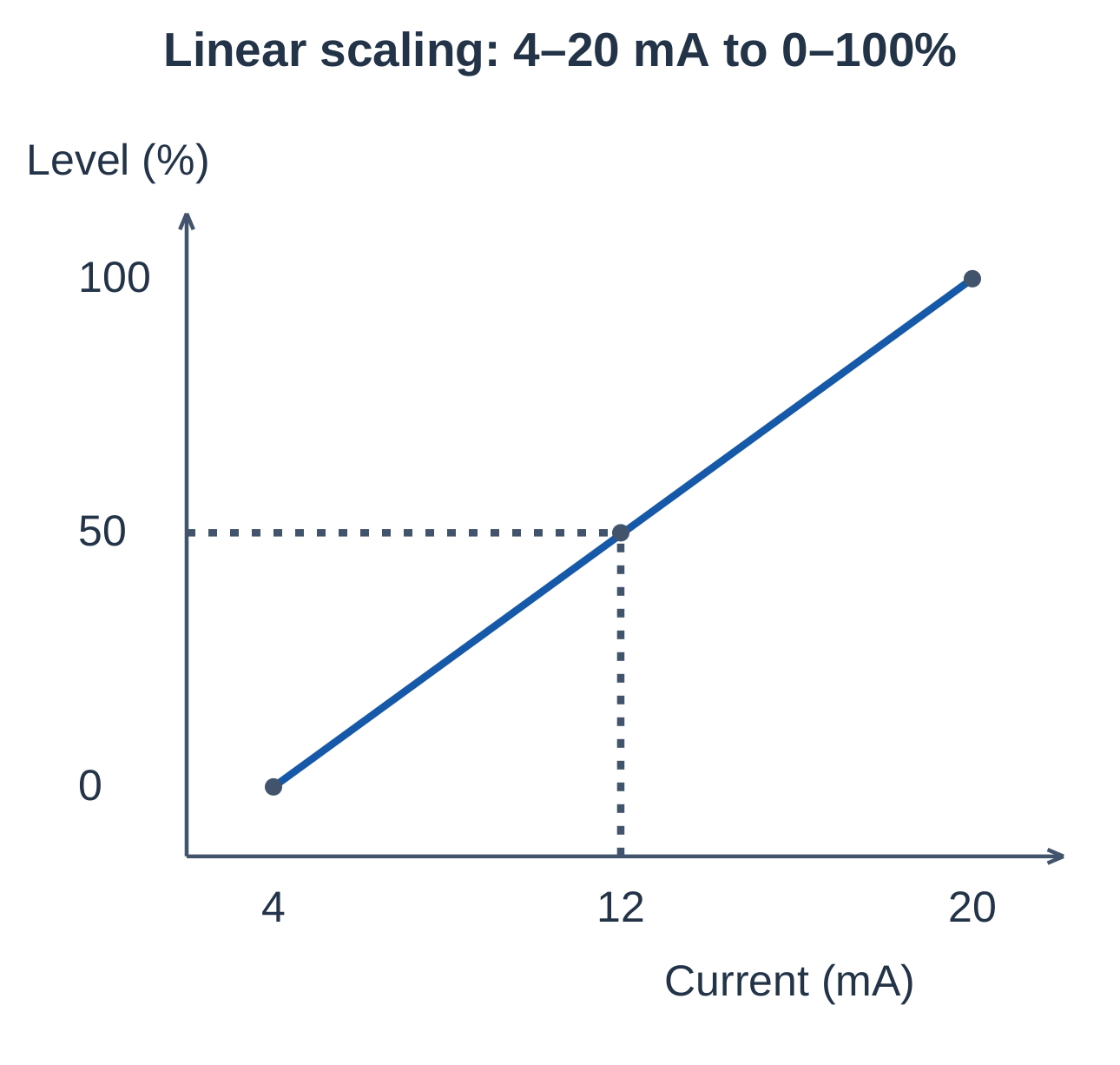
Example 2: Current to tank level
For an ideal 4–20 mA signal representing 0–100%, at 12 mA:
Level = [(12 − 4) / (20 − 4)] × 100 = 50%
Raw-count scaling and current scaling use different numerical endpoints even when they describe the same process quantity.
Analog Output
An analog output converts a programmed value into an electrical reference through a digital-to-analog output stage. The connected drive or valve must accept the selected range and common arrangement. A command value alone does not prove that the actuator reached the requested position.
3.4 Sinking and Sourcing Concepts
Sourcing supplies conventional current from the positive supply toward a connected circuit. Sinking receives current and provides its return toward 0 V or the negative side.
| Feature | Sourcing device | Sinking device |
|---|---|---|
| Current role | Supplies current from positive supply | Returns current toward 0 V |
| Typical DC sensor output | PNP | NPN |
| Usual matching PLC input | Sinking input | Sourcing input |
A complete loop must connect the supply, field output, input sensing circuit and common in the correct direction.
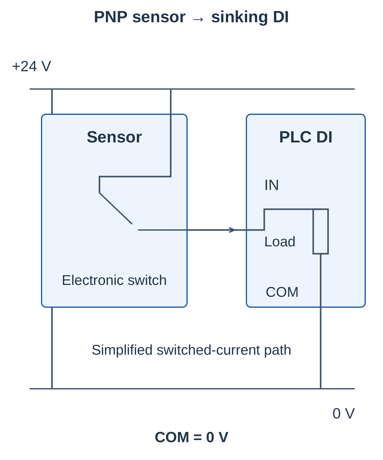
PNP Sensor with a Sinking Input
An active PNP output supplies current from +24 V toward the PLC input. The sinking input returns this current through its sensing circuit and common to 0 V.
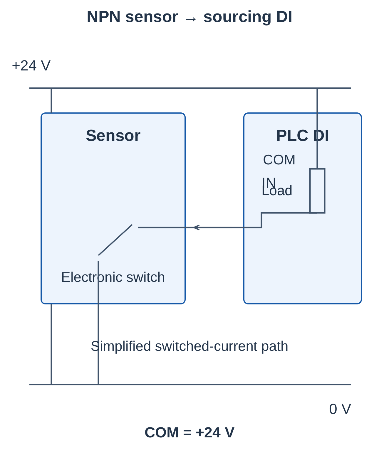
NPN Sensor with a Sourcing Input
A sourcing input supplies current from its positive common through the sensing circuit toward the input terminal. An active NPN output provides the return to 0 V.
Commons and Terminology
- State which device is being called sinking or sourcing.
- Some modules permit different arrangements through their common connection; others have a fixed design.
- Several points may share one common. Do not assume independent polarity or isolation for every point.
- Sinking and sourcing describe electrical current paths, not subtraction or software data sources.
- Conventional current direction is opposite to electron motion in a simple metal conductor.
3.5 Sinking and Sourcing Output Circuits
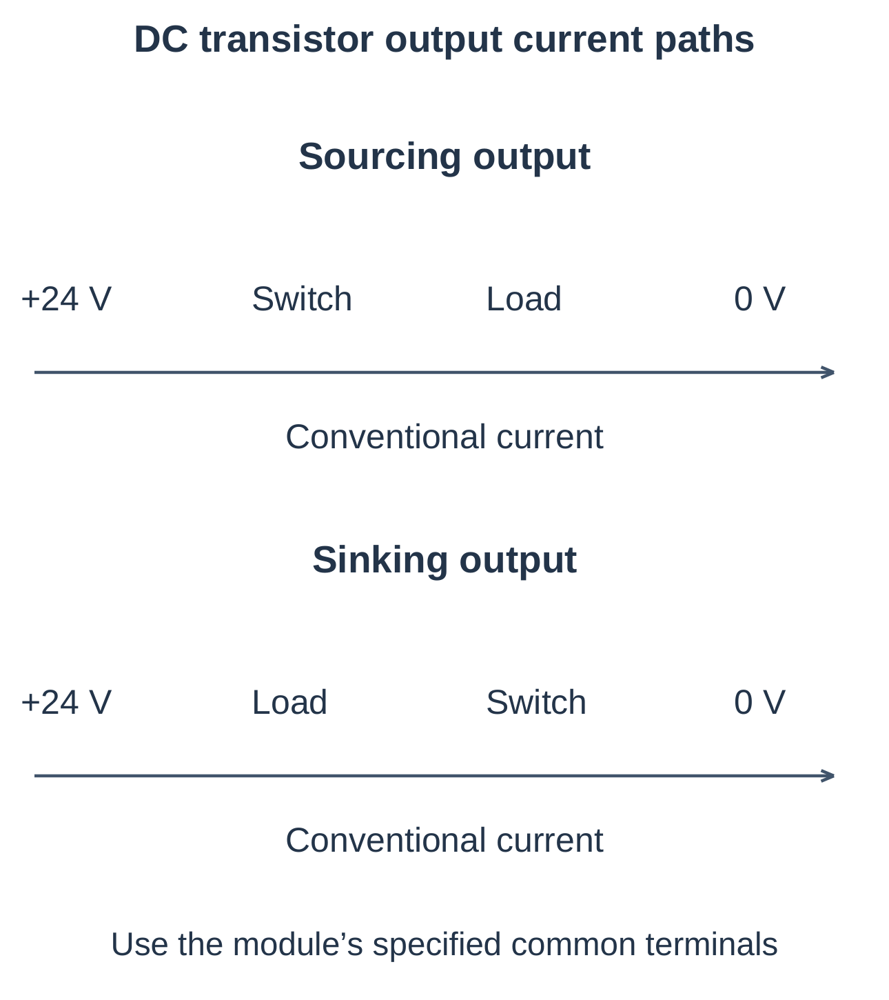
The same reasoning applies to transistor outputs operating DC loads.
| Feature | Sourcing PLC output | Sinking PLC output |
|---|---|---|
| Switched side | Positive supply side | Return side |
| Load connection | Output point to 0 V | Positive supply to output point |
| Enabled current path | Supply, output switch, load, 0 V | Supply, load, output switch, 0 V |
Interface Selection Steps
- Identify whether the field output sources or sinks current.
- Identify the PLC input’s current role.
- Trace the complete supply-to-return loop.
- Check commons, voltage, current and isolation.
- Confirm how the active electrical signal changes the program bit.
Worked Wiring Diagnosis
A PNP sensor appears active, but its PLC input does not change. Check sensor power, the signal terminal, the 0 V reference and whether the input supports sinking operation before editing the ladder program.
Also verify output voltage drop, leakage sensitivity and inductive suppression. A transistor output cannot automatically replace a relay output simply because their nominal supply voltages match.
3.6 Ladder Diagram Fundamentals
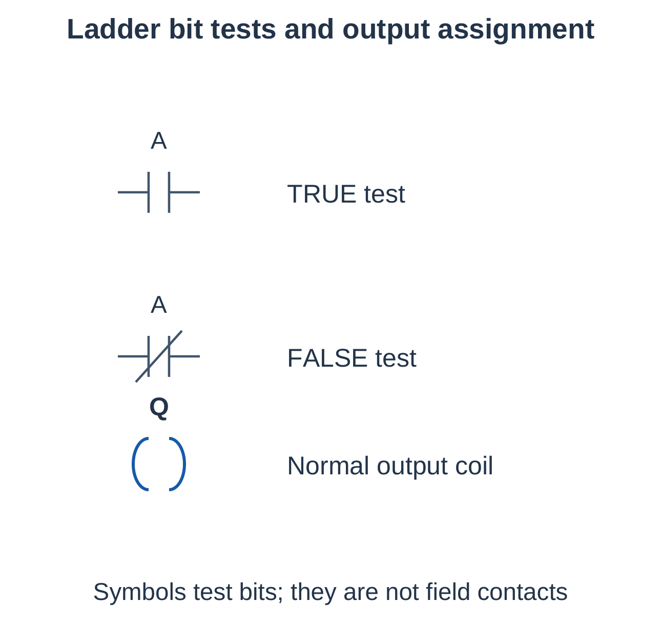
Ladder diagram, or LD, represents logical conditions and operations through rungs between graphical rails. Contact-style instructions test bits; coils assign results; function instructions perform operations.
The rails represent logical flow in the program. They are not field supply connections to the CPU.
TRUE and FALSE Tests
| Instruction | Logical continuity exists when |
|---|---|
| Test TRUE | Addressed bit = 1 |
| Test FALSE | Addressed bit = 0 |
| Normal output coil | Assigns its bit according to the executed rung result |
AND, OR and NOT Logic
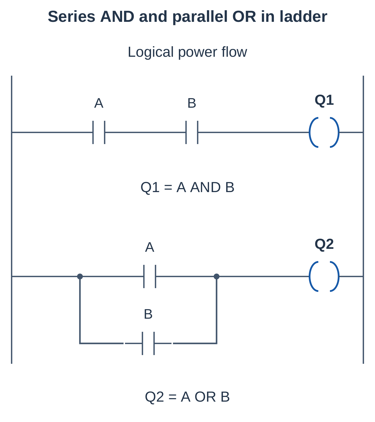
- Series conditions implement AND.
- Parallel branches implement OR.
- A FALSE test implements NOT of the addressed bit.
For Q = (A OR B) AND C, A and B form parallel branches, while C is in their common series path.
Evaluation, Tags and Coils
A typical rung evaluates conditions toward its output instructions. Rungs commonly execute in program order, subject to task scheduling and instruction behaviour.
Use descriptive tags such as StartPB, StopOK, RunCmd and TankLevel. Address formats vary by platform, so document the assignments used.
A normal coil assigns a bit whenever it executes. Set/reset or latch/unlatch instructions retain state differently and need defined reset, initialization and priority rules.
3.7 Ladder Programming: Start–Stop Memory
Input and State Assignment
| Tag | Meaning when TRUE |
|---|---|
| StartPB | Start button active |
| StopOK | NC stop circuit healthy and unpressed |
| OL_OK | Overload permission healthy |
| RunCmd | Stored running command |
Holding-Rung Equation
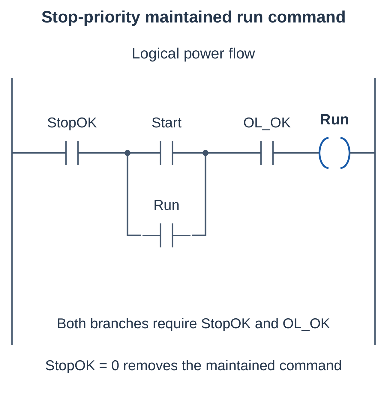
Place StopOK and OL_OK in the common series path. Place StartPB and RunCmd in parallel.
RunCmd(next) = StopOK AND OL_OK AND [StartPB OR RunCmd(previous)]
Operating Sequence
- With both permissions TRUE, pressing start makes RunCmd TRUE.
- Releasing start leaves the RunCmd holding branch TRUE.
- Pressing stop makes StopOK FALSE.
- Loss of StopOK or OL_OK breaks the common path and clears RunCmd when the rung executes.
The physical stop contact is NC, but the program tests StopOK for TRUE because TRUE means the stop circuit permits running.
Restart and Set/Reset Behaviour
A software holding bit’s startup value depends on memory configuration and initialization. Define the restart policy after power loss.
Set/reset instructions can provide another form of memory. If both commands occur together, execution order or instruction priority determines the result. Document the required reset priority.
3.8 Programming Practices and Scan Effects
Translate Requirements into Logic
- List physical inputs, outputs and internal states.
- Define what TRUE means for each signal.
- Specify permissions and stop behaviour.
- Identify timing and counting requirements.
- Write the logic with clear state ownership.
- Test normal operation, faults and recovery.
Avoid conflicting assignments to the same tag. A later executed normal assignment can overwrite an earlier result in the same cycle.
Rising-Edge Detection
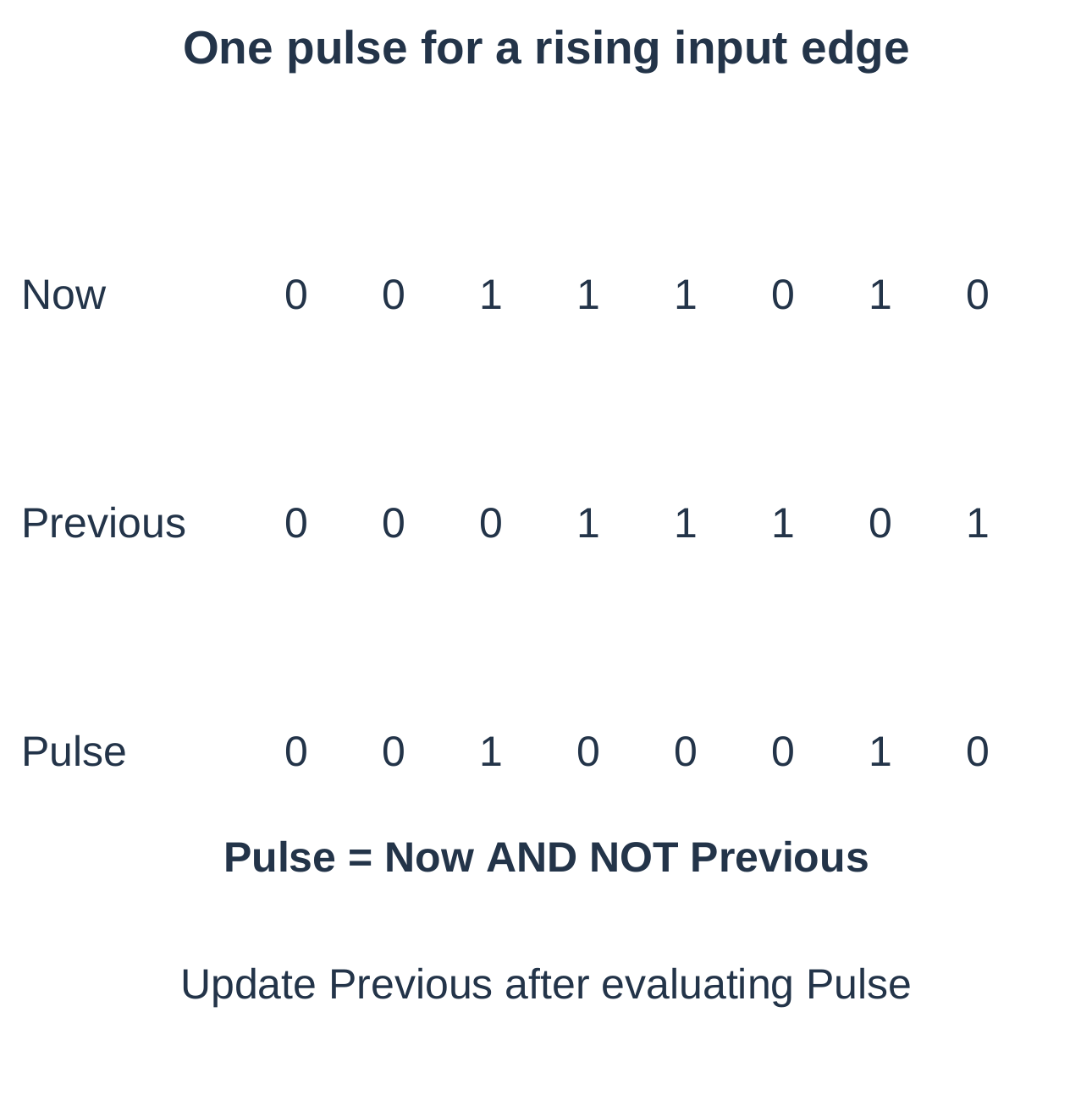
A rising edge is a FALSE-to-TRUE transition. A one-execution pulse can be defined as:
Pulse = Input(now) AND NOT Input(previous)
Update the previous-state memory after evaluating the pulse in the chosen execution arrangement.
Mechanical bounce can create several transitions for one intended event. Filtering or debouncing should reject unwanted changes without hiding valid events.
Program Verification Matrix
| Test | Expected verification |
|---|---|
| Normal start and stop | Correct command and state changes |
| Permission loss | Defined output response |
| Input held TRUE | No unintended repeated event action |
| Short pulse | Event captured or limitation identified |
| Reset with active command | Correct priority and recovery |
| Power or network recovery | Defined initialization and data quality |
3.9 Sequential Function Chart
A sequential function chart, or SFC, organizes operation into steps, transition conditions and actions. It gives a more specific sequence model than a general-purpose flowchart.
| Element | Meaning |
|---|---|
| Initial step | Starting stage of the sequence |
| Step | A process stage that can be active |
| Transition | Condition permitting progression |
| Action | Work associated with an active step |
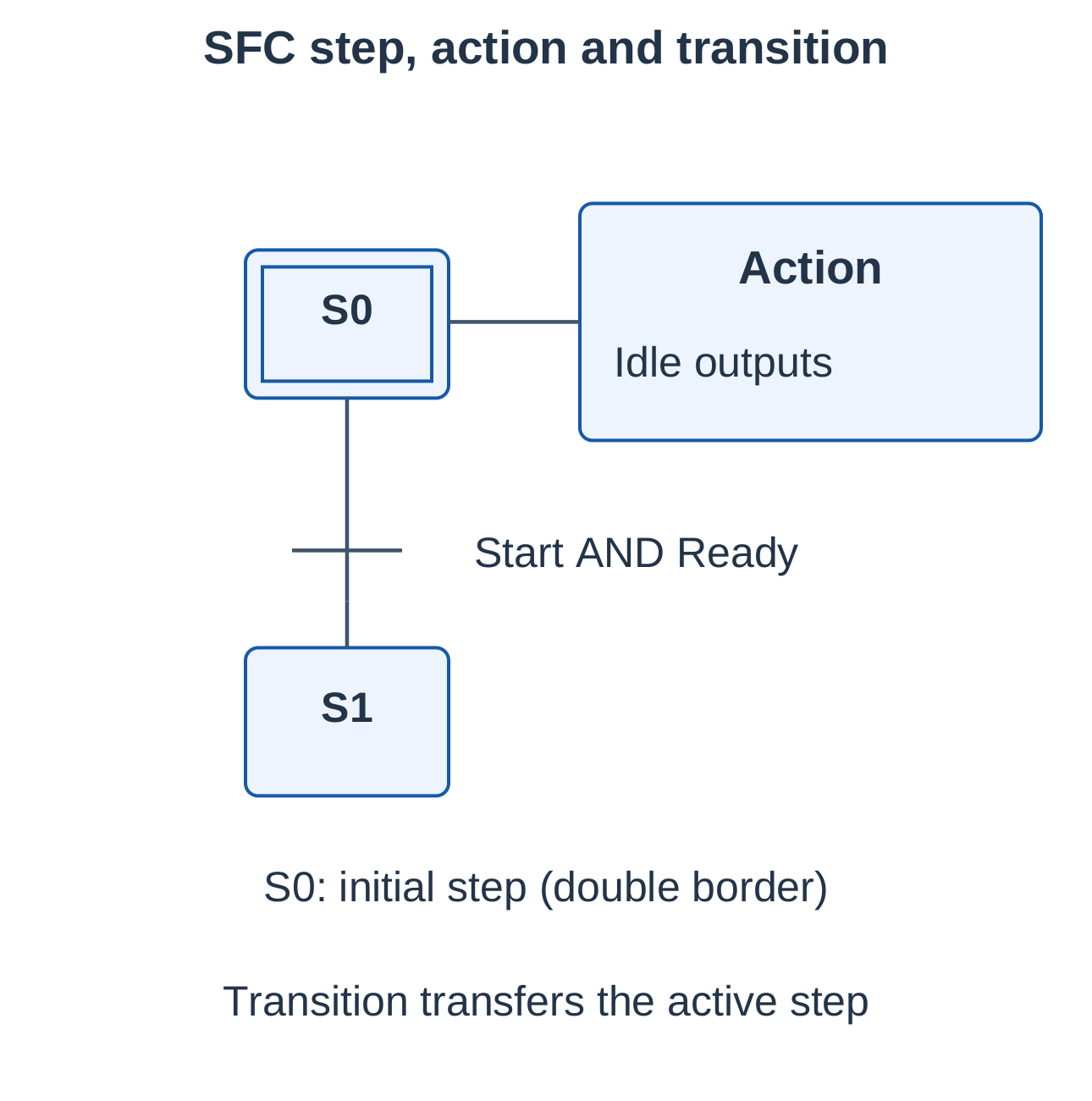
A transition can fire when its preceding steps are active and its condition is satisfied. The chart structure determines which steps become inactive and which become active.
Output behaviour depends on the action definition and qualifiers. An action is not automatically retained after its step ends, nor does every qualifier necessarily clear every output.
Ladder Diagram and SFC Comparison
| Feature | Ladder diagram | SFC |
|---|---|---|
| Main organization | Boolean rungs and instructions | Steps, transitions and actions |
| Strong application | Interlocks and Boolean logic | Staged operating sequences |
| Sequence memory | Internal tags or state logic | Step activity |
| Combined use | Implements conditions and actions | Can use ladder for associated logic |
Define the initial state, reset destination and fault recovery. Returning to the initial step is insufficient if actuators or retained actions remain inconsistent with it.
3.10 SFC Example: Fill, Hold and Drain
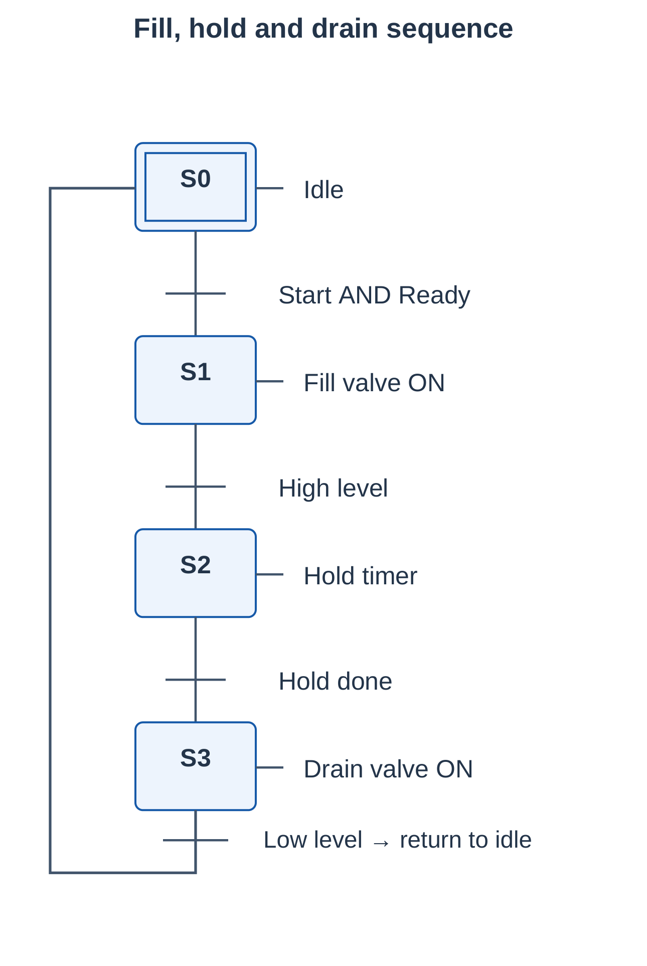
The required process starts idle with both valves closed, fills to high level, waits for a defined interval, drains to low level and returns to idle.
| Step | Action | Transition |
|---|---|---|
| S0: Idle | Both valves closed | Start AND Ready |
| S1: Fill | Inlet commanded ON | High level reached |
| S2: Hold | Valves closed; timer active | Hold interval complete |
| S3: Drain | Outlet commanded ON | Low level reached; return to S0 |
Outputs must also satisfy the required machine permissions. Define responses to contradictory level signals, timeouts, unavailable actuators and interrupted operation. Fault or Manual states may be needed.
Alternative and Simultaneous Branches
An alternative branch selects one path. Define priority or mutual exclusion when more than one transition can be TRUE.
A simultaneous branch activates parallel sequences. Its join must wait for the stated completion conditions.
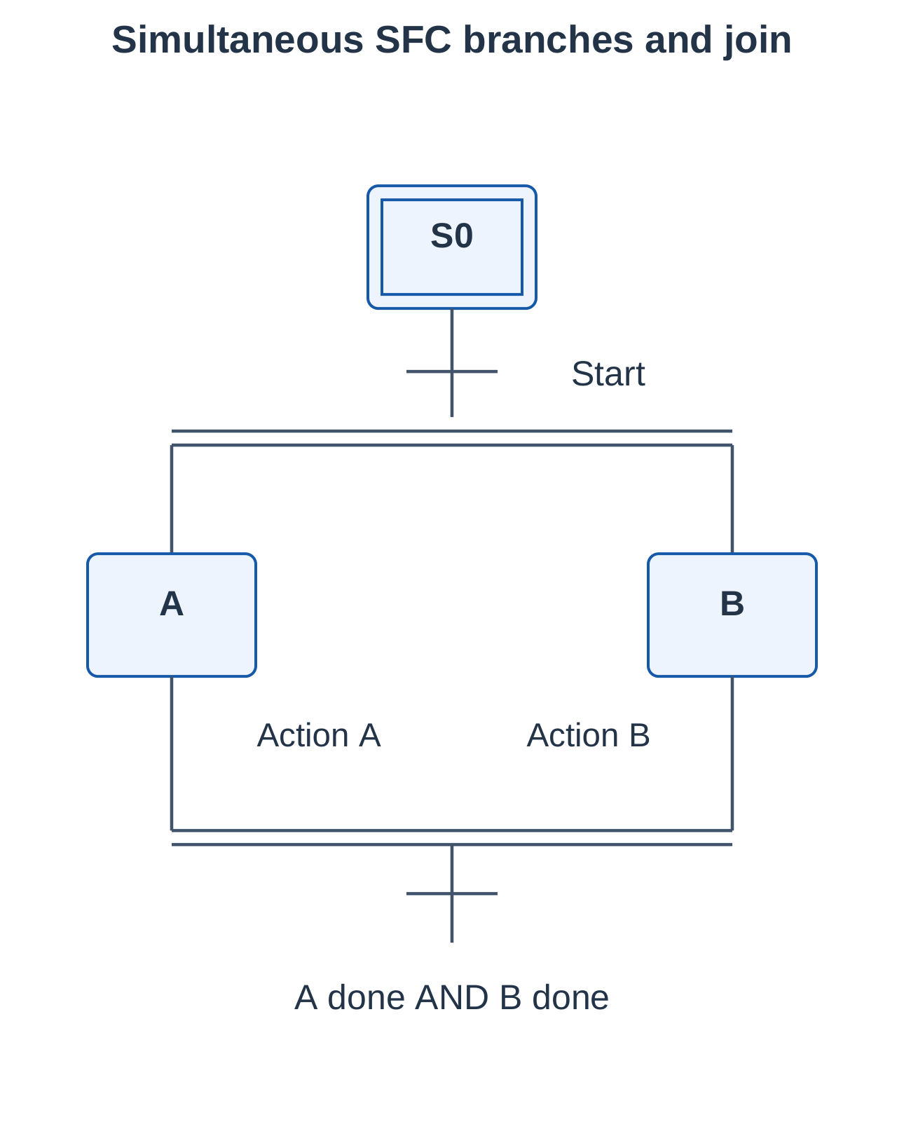
Ladder can implement the same sequence using state bits or an integer state tag. Maintain intended state exclusivity and clear entry, exit and recovery rules.
3.11 Timer Instruction Foundation
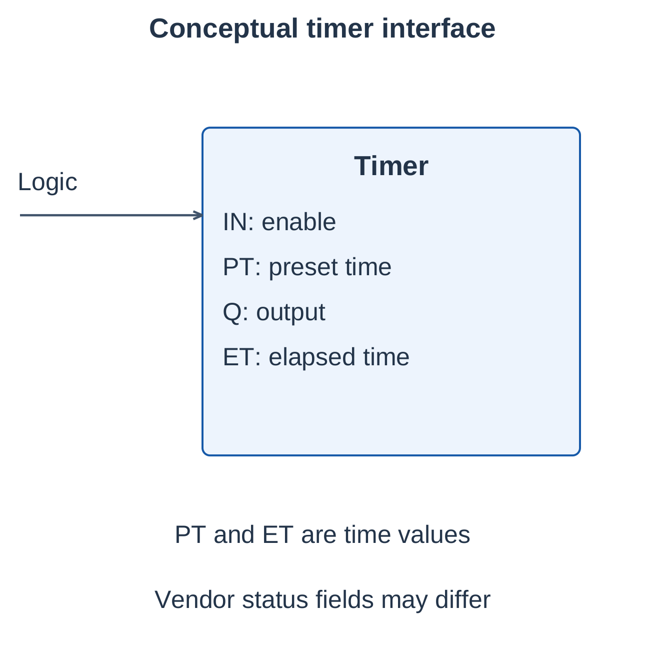
A PLC timer connects a controlling condition to elapsed time and an output condition. It is a software instruction rather than necessarily a separate timing relay.
| Parameter | Meaning |
|---|---|
| IN or enable | Timing control condition |
| PT or preset | Required time interval |
| ET or accumulated value | Elapsed time under the instruction’s rules |
| Q or completion output | Defined timer output condition |
| Reset | Clears retained state where applicable |
Time Base
For a count-based timer:
Requested time = Preset count × Time base
A 5 s interval with a 10 ms base requires:
Preset count = 5 / 0.01 = 500
Some implementations accept a time value directly. Physical response also depends on task execution, input capture, output updating and actuator behaviour.
Use separate timer instances for unrelated operations. Reusing one timer structure through conflicting paths can change its elapsed value and status unexpectedly.
3.12 On-Delay Timer: TON
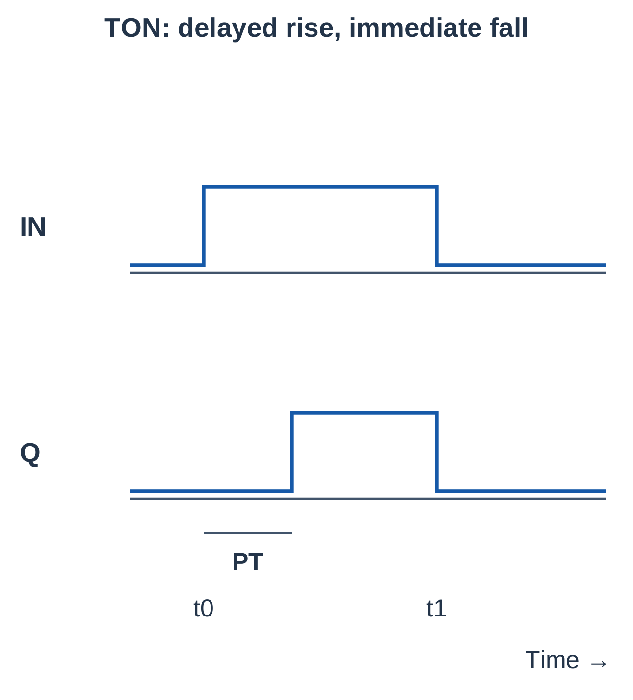
A non-retentive TON delays the rising edge of Q.
- IN becomes TRUE and timing starts.
- IN must remain continuously TRUE for PT.
- Q becomes TRUE when the qualifying interval completes.
- IN becoming FALSE clears Q and elapsed time in this model.
Fan-Proof Example
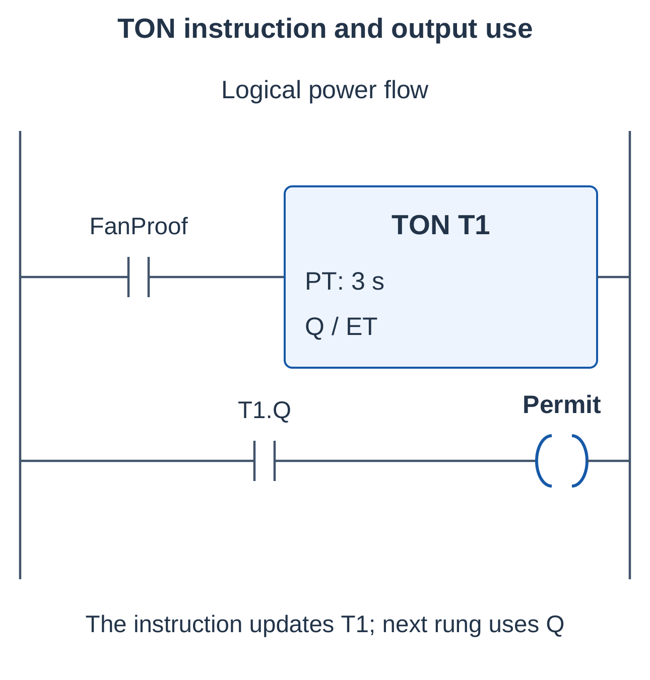
A fan-run proof must remain TRUE for 3 s before a conveyor permission is granted. FanProof enables TON T1 with PT = 3 s. A separate test of T1.Q supplies Permit.
Interrupted Timing Example
PT = 5 s. IN is TRUE for 2 s, FALSE for 1 s and TRUE again for 5 s. The first 2 s are discarded. Q becomes TRUE after the later uninterrupted 5 s interval.
An input pulse shorter than PT does not generate the delayed-on output in this model.
Common errors include using the input instead of Q for the delayed action, assuming retention after IN falls, mixing time units and sharing one timer between unrelated operations.
3.13 Off-Delay Timer: TOF
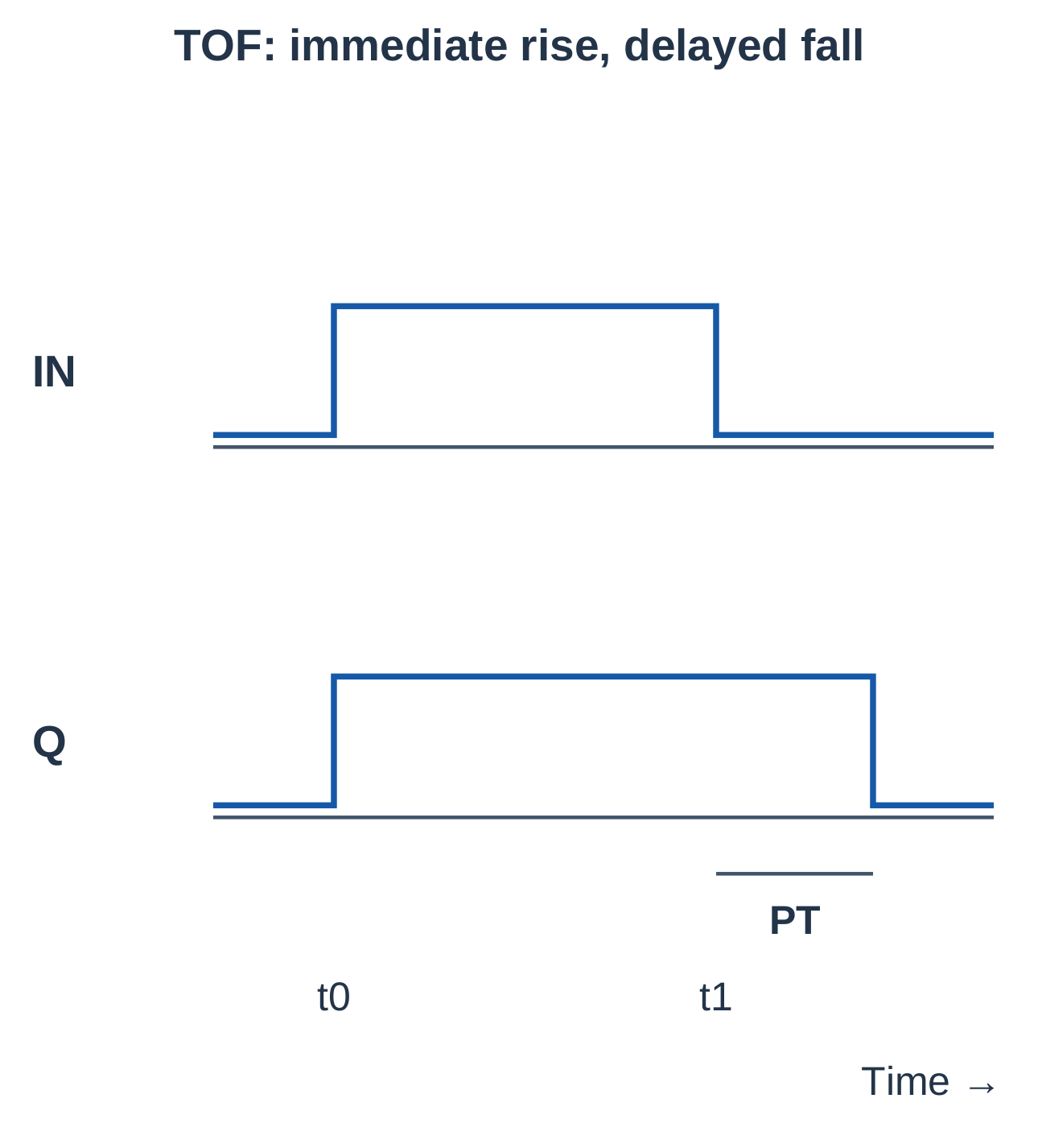
A TOF delays the falling edge of Q.
- While IN is TRUE, Q is TRUE.
- When IN becomes FALSE, the off-delay begins.
- Q remains TRUE for PT.
- Q becomes FALSE when that interval finishes.
If IN returns TRUE before expiry, Q stays TRUE and the falling-delay sequence is cancelled or reinitialized according to the instruction model.
Extraction-Fan Example
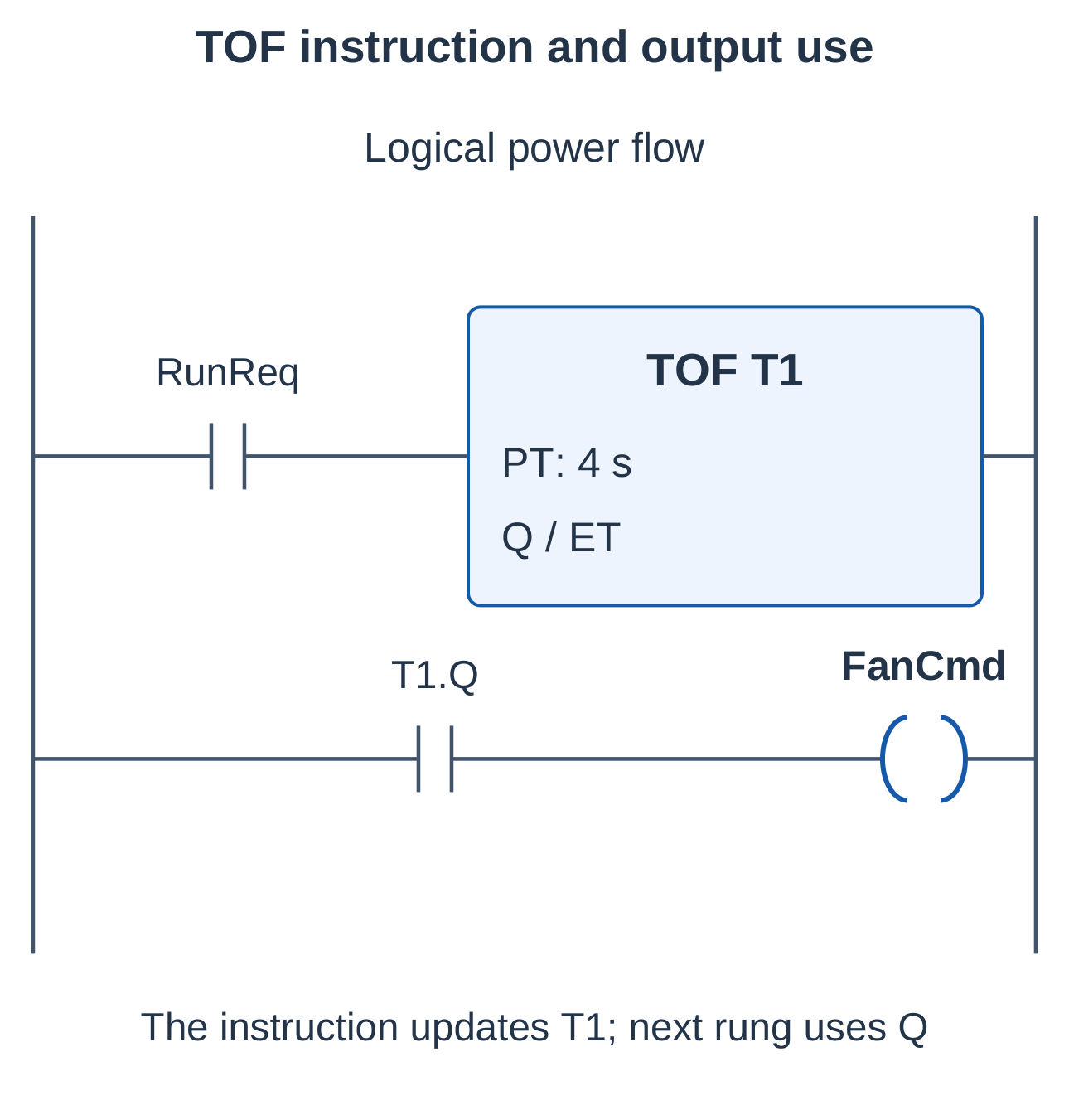
An extraction fan must run for 4 s after RunRequest disappears. RunRequest enables the TOF; its delayed-falling Q provides FanCmd through the required permission logic.
Worked Timing Example
IN is TRUE from t = 0 to t = 10 s, with PT = 4 s. Q stays TRUE until approximately t = 14 s in the ideal model.
A TOF status bit called “done” may remain TRUE during the input-on and delay periods, then clear at expiry. Interpret the actual instruction rather than assuming every done bit rises at the end of timing.
A delayed process stop must not unintentionally delay a stop that requires immediate command removal. Permission placement must reflect the required stopping behaviour.
3.14 Retentive Timer
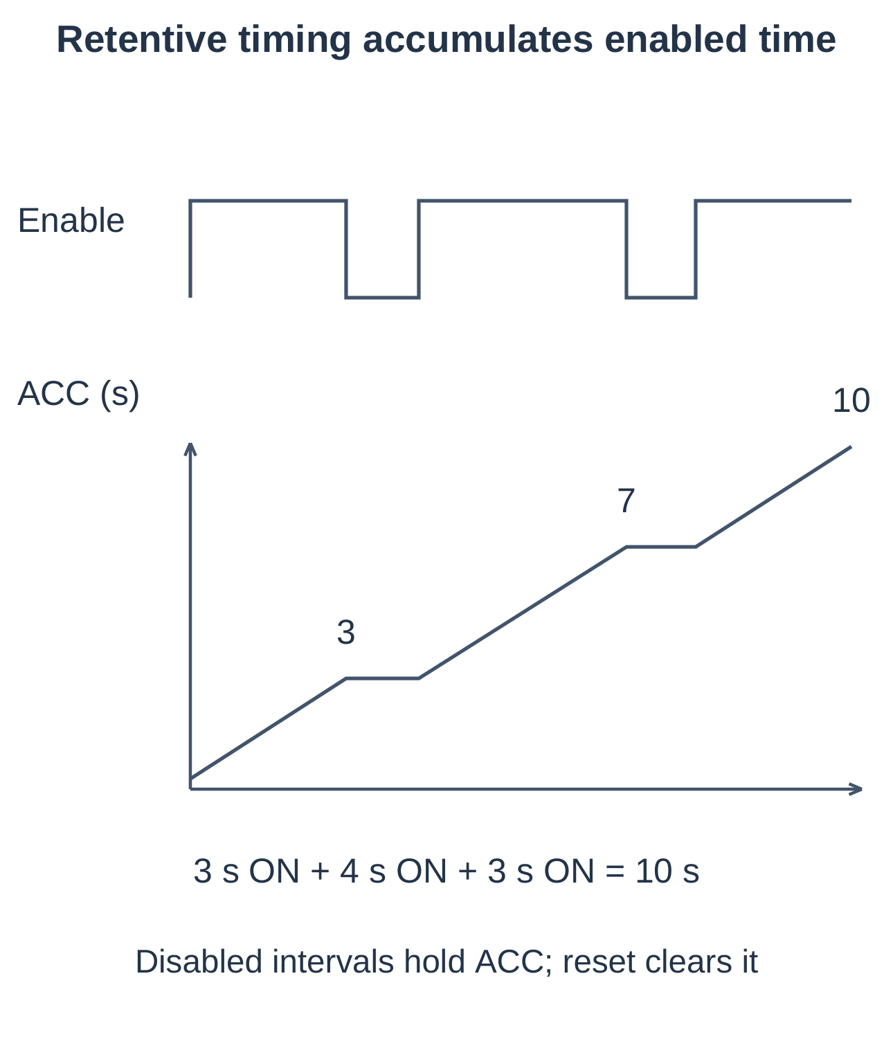
A retentive timer accumulates enabled operating time across interruptions. In the illustrated model, disabling the input holds the accumulated value; a separate reset clears it.
Worked Example
For PT = 10 s, enabled intervals of 3 s, 4 s and 3 s give:
Accumulated enabled time = 3 + 4 + 3 = 10 s
Completion occurs during the third interval. Disabled intervals do not contribute to the total.
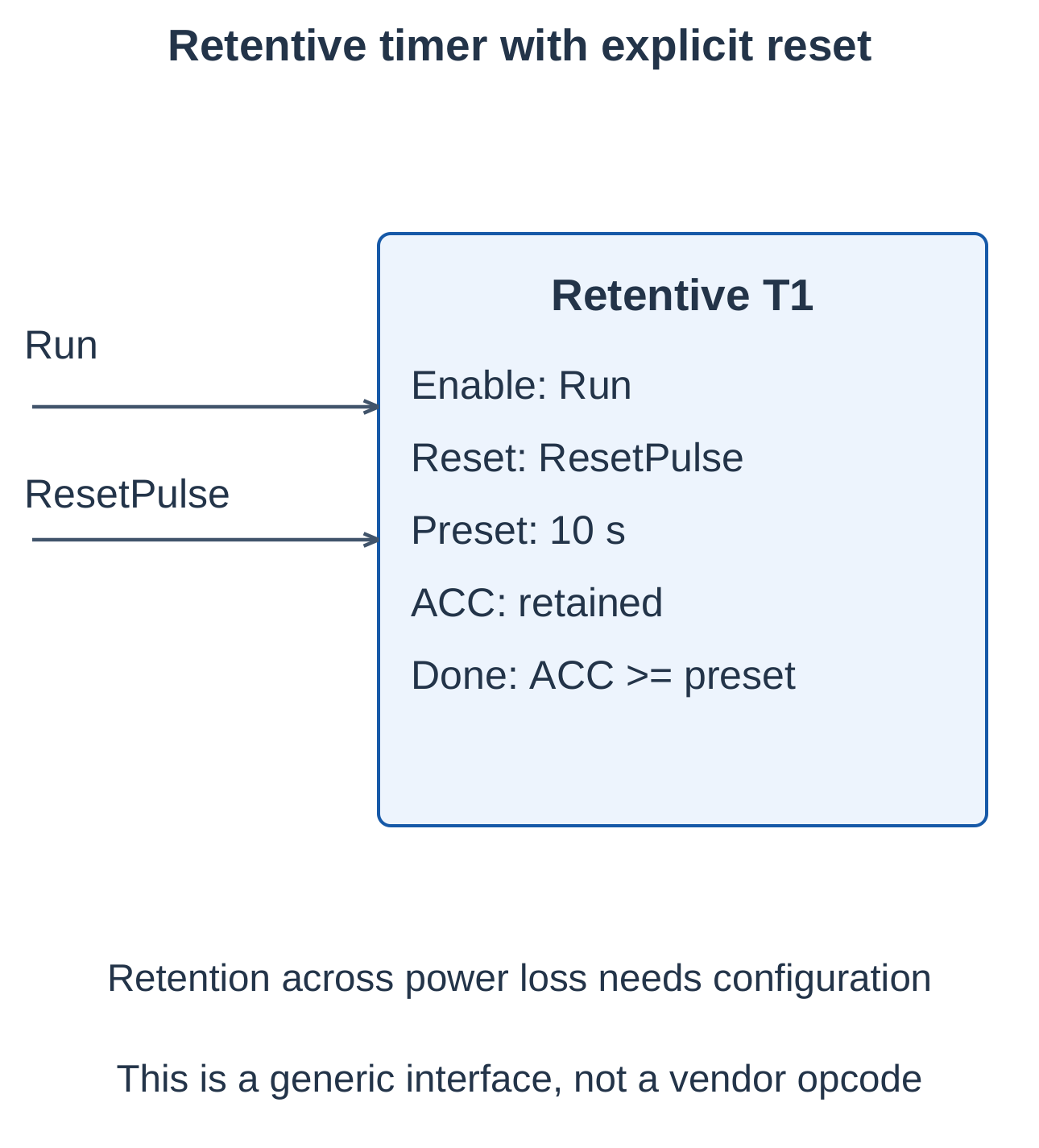
TON and Retentive Timer Comparison
| Feature | Non-retentive TON | Retentive model |
|---|---|---|
| Input becomes FALSE | Elapsed value resets | Accumulated value remains |
| Later enable | Starts a new interval | Continues accumulation |
| Clearing time | Normal disabling resets it | Explicit reset required |
| Application | Continuous-condition delay | Cumulative run-time monitoring |
Retention during input interruption does not guarantee retention through power loss, restart, memory clear or program download.
For maintenance monitoring, define actual operation carefully. A motor command alone may not establish that the motor ran; use suitable feedback where actual operating time is required.
3.15 Cyclic Timers and Repeating Operation
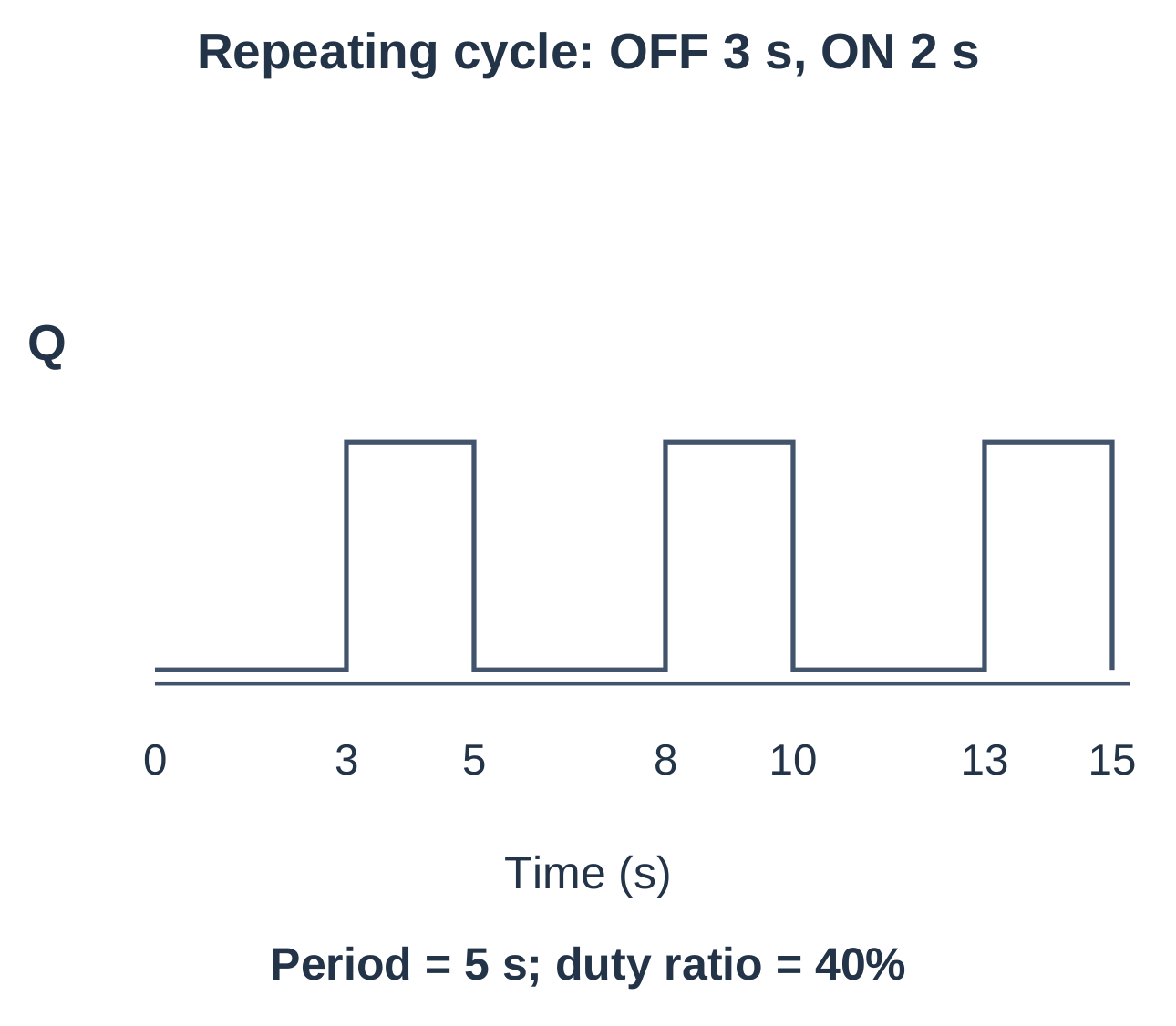
A cyclic timing function repeatedly alternates between defined ON and OFF states while enabled. It can use a dedicated instruction or timer-based state logic. Parameter names and mnemonics vary across PLCs.
Cyclic Timing Relationships
Period T = T_on + T_off
Frequency f = 1 / T
Duty cycle = (T_on / T) × 100%
For a lamp ON for 2 s and OFF for 3 s:
- Period = 5 s.
- Frequency = 0.2 Hz.
- Duty cycle = 40%.
Two-State Implementation
- Initialize to OFF and keep the lamp command FALSE.
- Run the OFF timer for 3 s.
- Change to ON when the OFF interval completes.
- Command the lamp and run the ON timer for 2 s.
- Return to OFF when the ON interval completes.
- Reset inactive timing state according to the instruction’s behaviour.
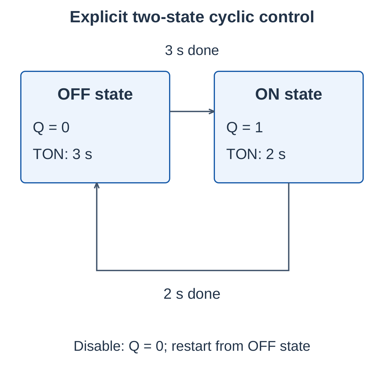
In this example, disabling removes the lamp command and re-enabling starts a fresh OFF phase.
Ordinary task-based transitions include execution latency. For precise pulse generation, select suitable hardware or high-speed facilities. An unexplained self-resetting timer rung may create a one-scan pulse or implementation-dependent oscillation.
3.16 Timer Selection and Timing Problems
| Requirement | Timer concept |
|---|---|
| Wait before enabling an output | TON |
| Keep output ON after input falls | TOF |
| Accumulate time over separate runs | Retentive timing |
| Repeat defined ON/OFF phases | Cyclic timing |
TON and TOF Comparison
| Feature | TON model | TOF model |
|---|---|---|
| Delayed output edge | Rising | Falling |
| IN becomes TRUE | Qualifying interval starts | Q becomes TRUE |
| IN becomes FALSE | Q clears and elapsed resets | Off-delay starts |
| Typical use | Delayed permission | Fan overrun |
Worked Time-Base Problem
Preset count = 250 and time base = 20 ms:
Time = 250 × 20 ms = 5000 ms = 5 s
For an 8 s interval with the same base:
Preset count = 8000 / 20 = 400
Worked TOF Reactivation
PT = 4 s. IN falls at 10 s, then returns TRUE at 12 s. The delay has not expired, so Q remains TRUE. A later falling input begins another off-delay under this model.
Verify short enables, threshold crossing, reactivation, reset during timing and reset while enable remains TRUE. State units and the assumed instruction model.
3.17 Counters and Pulse Interpretation
A software counter changes a numerical value in response to recognized events. Common PLC counters respond to rising edges, not every scan containing a TRUE input.
| Parameter | Meaning |
|---|---|
| CU / CD | Up-count / down-count event input |
| PV | Threshold or preset value to load |
| CV | Current count |
| R | Reset, where defined |
| LD | Load preset into a down-counter |
| Q | Status defined by the counter model |
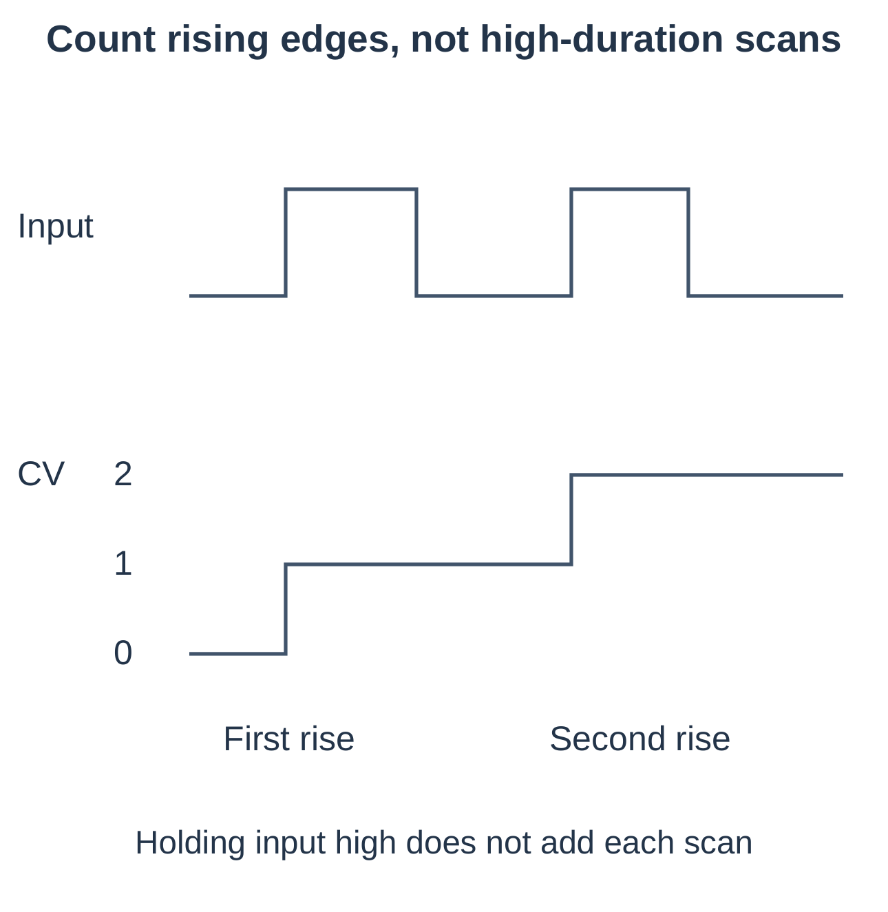
One carton holding a sensor TRUE for six scans should normally generate one event. Another event requires a recognized return to FALSE followed by a new rising edge.
Define priority when reset or load coincides with a count edge. These examples use reset priority for CTU and load priority for CTD. Check counting frequency, numerical range and overflow behaviour as well as the input circuit.
Accurate counting depends on event capture, pulse width, bounce control and the meaning assigned to each detected transition. Ordinary scanning may miss fast events; a high-speed counter or other capture facility may be necessary.
3.18 Up-Counter: CTU
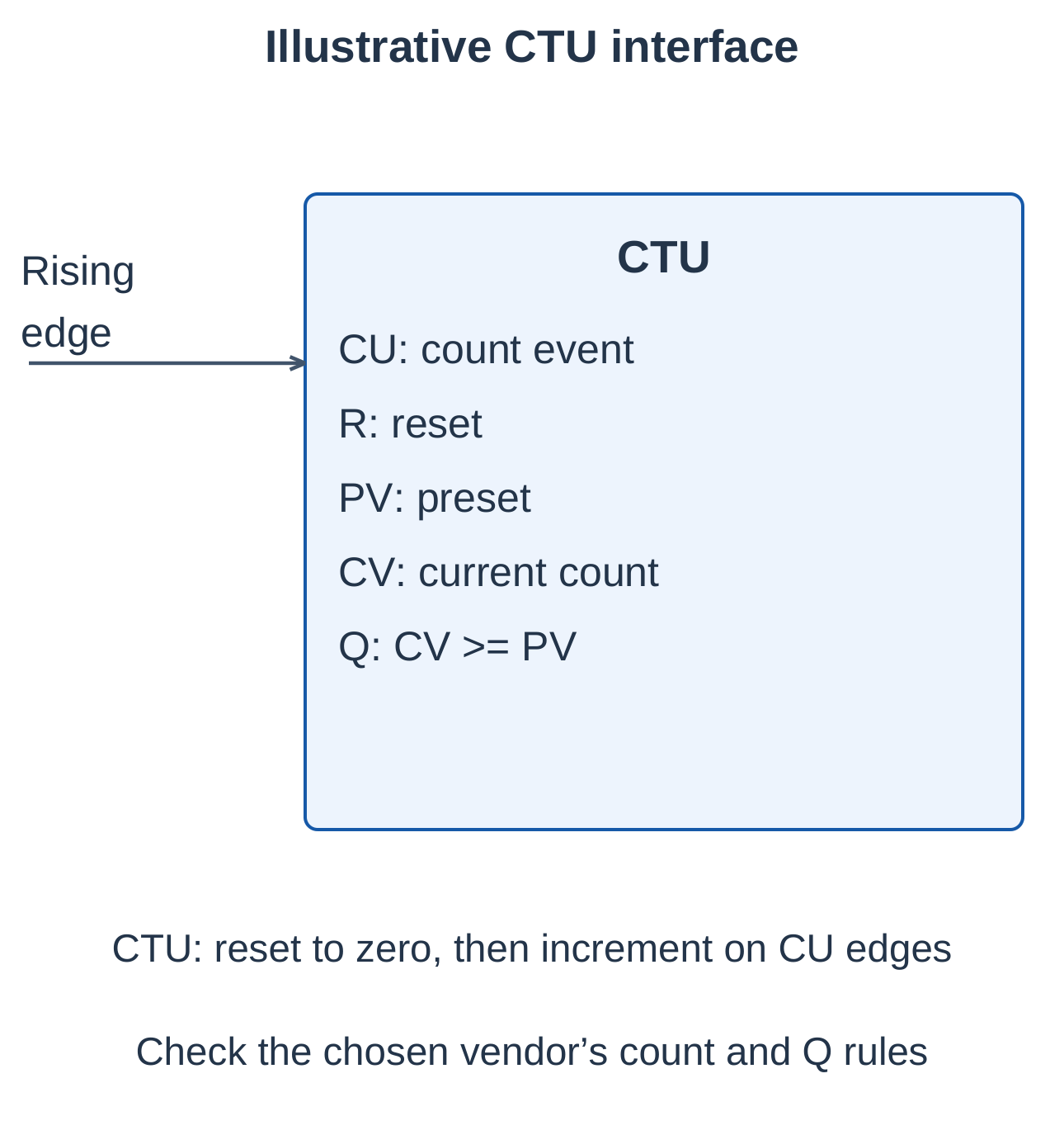
In the illustrative IEC-style CTU model, each recognized rising edge at CU increments CV. Reset clears the count. Q indicates CV ≥ PV within the instruction’s defined range.
Five-Carton Worked Example
With PV = 5 and CV initially zero, five distinct sensor rising edges give counts 1, 2, 3, 4, 5. At CV = 5, Q becomes TRUE and can request BatchComplete. Reset clears CV and Q in this simplified model; count edges are accepted while reset is inactive.
Ten-Part Batch
Set PV = 10. Each recognized part event increments CV. When CV reaches 10, the program can use the completion condition to remove feed permission and indicate BatchReady.
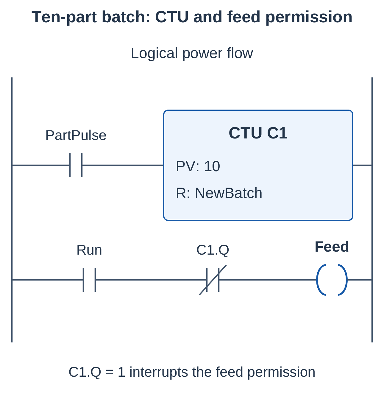
Q becoming TRUE does not universally stop counting. Define whether additional events are accepted, inhibited, limited or followed by a reset.
Held-Input Example
For sensor samples 0, 1, 1, 1, 0, 1, there are two rising edges. The count increases by two if both events are recognized. Repeated TRUE samples do not represent repeated new events.
3.19 Down-Counter: CTD
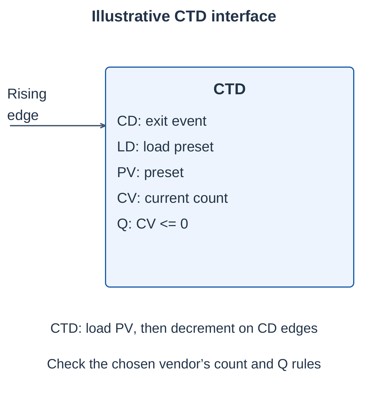
In the illustrated IEC-style CTD model:
- LD loads PV into CV.
- Each recognized rising edge at CD decrements CV while load is inactive.
- Q indicates CV at or below zero according to the instruction’s defined limits.
Remaining-Items Example
Load PV = 4. Four recognized dispensing events produce CV values 3, 2, 1, 0. At zero, Q becomes TRUE in this model. The program can then inhibit dispensing or request refill.
Loading a preset is different from resetting to zero. Holding LD TRUE in a load-priority model can reload the quantity every execution and prevent intended counting.
CTU and CTD Comparison
| Feature | CTU example | CTD example |
|---|---|---|
| Event input | Rising edge at CU | Rising edge at CD |
| Count direction | Increasing | Decreasing |
| Initialization | Reset to zero | Load PV into CV |
| Completion | CV reaches PV | CV reaches zero |
| Typical interpretation | Items produced | Items remaining |
Some controller families use different CTU/CTD accumulated values and status-bit rules. Do not transfer zero-detection or done-bit equations unchanged between platforms.
3.20 Up/Down Counting and Application Design
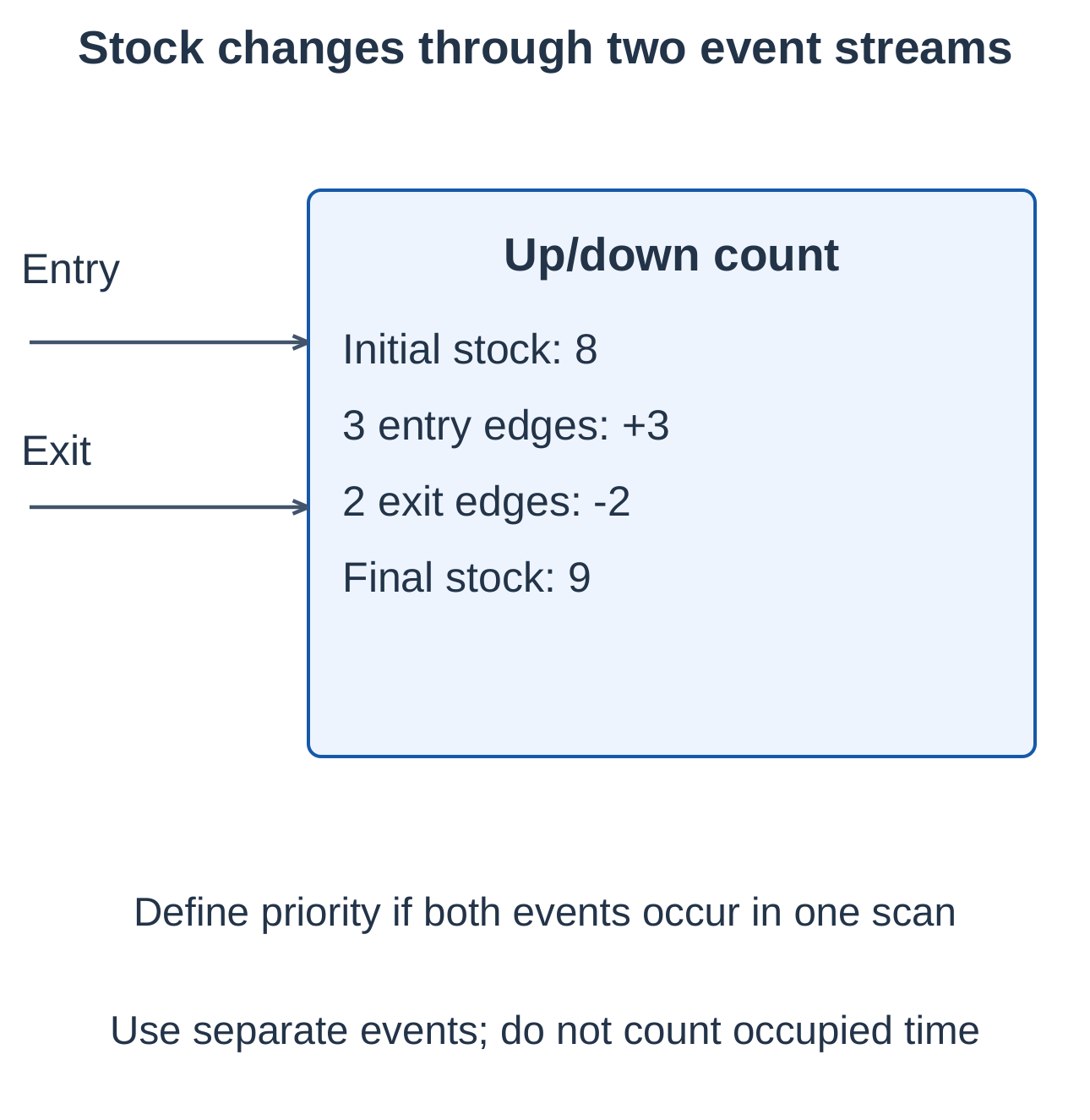
An up/down counter tracks additions and removals, such as stock, occupancy or parts in a buffer.
New count = Old count + Accepted entry events − Accepted exit events
With initial stock 8, three entries and two exits:
New stock = 8 + 3 − 2 = 9
Simultaneous Events and Bounds
Define how simultaneous entry and exit events are handled. A no-net-change policy must be supported by the selected instruction or implemented explicitly.
Prevent or diagnose negative stock and quantities above physical capacity. Reset should establish a verified starting condition. Missed, repeated or bypassed events can cause drift and require reconciliation.
Counter and Timer Comparison
| Feature | Counter | Timer |
|---|---|---|
| Measures | Recognized events | Elapsed time under stated conditions |
| Main trigger | Input transitions | Timing enable or edge condition |
| Units | Parts, cartons or cycles | Seconds or milliseconds |
| Common mistake | Counting scans instead of events | Incorrect time base or retention assumption |
3.21 Math Instructions and Numerical Data
Math instructions calculate measurements, quantities and commands. Exact instruction names and operand rules depend on the platform.
| Operation | Illustrative expression |
|---|---|
| ADD | Destination = A + B |
| SUB | Destination = A − B |
| MUL | Destination = A × B |
| DIV | Destination = A / B, provided B is valid and nonzero |
Data Types and Integer Division
Integers represent whole numbers within a finite range. Real or floating-point values permit fractions with finite precision. Signedness, conversions and intermediate-result types affect the answer.
In a truncating integer-division model:
7 / 2 = 3
With suitable real arithmetic:
7 / 2 = 3.5
A real destination alone does not necessarily make earlier intermediate calculations real.
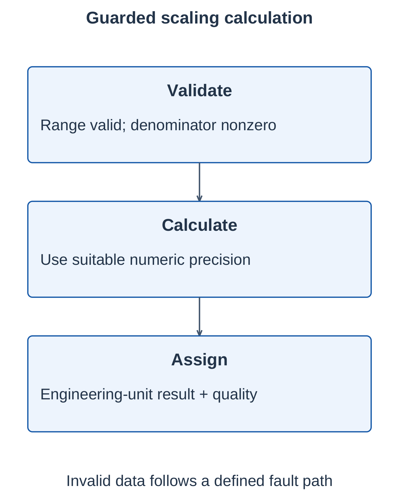
Scaling Order and Error Handling
For raw 0–4000 mapped to 0–100%, integer division of Raw / 4000 first can produce zero across much of the range. Multiplying first can preserve more information but may overflow. Use a correctly sized or real intermediate.
Before calculation, check:
- Operand and intermediate types.
- Numerical ranges and overflow risk.
- Units and conversion factors.
- A valid, nonzero denominator.
- Destination type and result validity.
Define an error response for invalid arithmetic rather than executing division by zero or assuming overflow behaves identically on every PLC.
3.22 Comparison, Scaling and Worked Math Problems
Comparisons create Boolean conditions from numerical values. Examples include Level ≥ 80% and Count ≥ 20. The comparison supplies a condition; separate control logic determines the actuator command.
Use hysteresis or state logic when noise near a threshold would cause repeated switching.
Example 1: Pressure Scaling
Raw 1000–5000 represents pressure 0–10 bar. At Raw = 3400:
Pressure = [(3400 − 1000) / (5000 − 1000)] × 10 = 6 bar
Example 2: Production Rate
A machine produces 120 parts in 2 minutes:
Rate = 120 / 2 = 60 parts/min
Using 120 s instead:
Rate = (120 / 120) × 60 = 60 parts/min
Keep the time units consistent.
Example 3: Average Temperature
For readings of 24°C, 26°C and 28°C:
Average = (24 + 26 + 28) / 3 = 26°C
For a variable number of valid readings N, calculate only when N > 0. Define the result when no readings are valid.
Example 4: Rejection Percentage
Rejected parts = 9; total inspected = 300:
Rejection percentage = (9 / 300) × 100 = 3%
Use suitable precision and guard the total against zero.
Result Quality
Check measurement quality before displaying a precise-looking value. Define whether out-of-range data is clamped, alarmed, substituted or handled as a fault. Arithmetic alone cannot establish sensor validity.
3.23 Integrated PLC Example: Carton Batching
Requirement
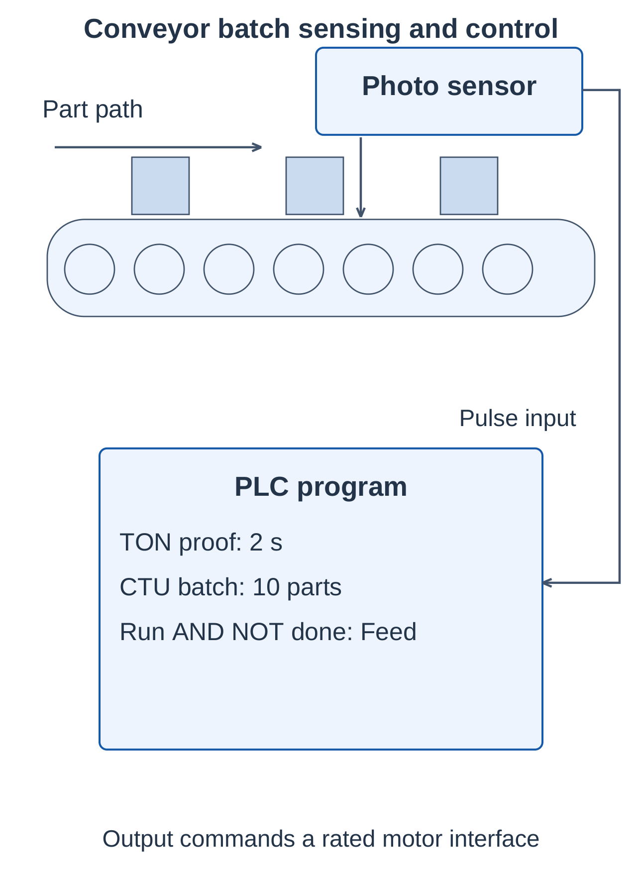
Start a conveyor only with valid StopOK and drive permissions. Qualify drive-run proof continuously for 2 s. Count 10 distinct carton detections, then stop feeding and indicate BatchReady. Reset prepares another batch under defined operating conditions.
Functional Allocation
| Function | Signals or instruction |
|---|---|
| Digital inputs | StartPB, StopOK, DriveOK, DriveRunProof, CartonSensor, ResetPB |
| Digital outputs | ConveyorCmd and BatchReady indicator |
| Internal states | RunRequest, qualified permission and batch state |
| Timer | TON with PT = 2 s for run-proof qualification |
| Counter | CTU with PV = 10 for recognized carton edges |
Program Sequence
- Evaluate operating permissions and reset conditions.
- Establish RunRequest from an allowed start.
- Qualify continuous drive-run proof using TON.
- Enable the conveyor under the intended state and permissions.
- Accept carton events while counting is permitted.
- On count completion, end feeding and indicate BatchReady.
Fault and Recovery Checks
- Missing drive proof must prevent the intended feed permission.
- A sensor held TRUE must not generate ten counts by repeated scanning.
- Reset must not silently produce an unexpected running command.
- Stop handling must interrupt the required output path even if timer or counter values remain stored.
Trace start, a held sensor, permission loss, the ninth carton, the tenth carton, extra events, reset and recovery. Define whether reset clears RunRequest as well as the count.
3.24 Quick Revision and Examination Practice
Essential Revision Points
- DI/DO carry discrete states; AI/AO carry variable measurements and commands.
- Sourcing provides current; sinking returns it toward 0 V.
- Typical PNP sensor outputs match sinking inputs; NPN outputs match sourcing inputs.
- Physical contacts establish input states; ladder contacts test stored bits.
- Series and parallel ladder paths implement AND and OR.
- A holding branch maintains a command while common permissions remain TRUE.
- SFC organizes steps, actions and transition conditions.
- TON delays a rising output; TOF delays a falling output.
- Retentive timing accumulates enabled time across input interruptions.
- Cyclic timing requires defined ON/OFF phases and initialization.
- Counters commonly respond to edges rather than every TRUE scan.
- Math needs suitable types, ranges, units and guarded calculations.
Important Formulas
| Relationship | Application |
|---|---|
| Time = Preset count × Time base | Count-based timer setting |
| T = T_on + T_off | Cyclic period |
| f = 1 / T | Cycle frequency |
| Duty = (T_on / T) × 100% | ON percentage |
| Scaled value = E_min + (Raw − R_min) × E_span / R_span | Linear scaling |
| New stock = Old stock + Entries − Exits | Inventory counting |
| Pulse = Now AND NOT Previous | Rising-edge detection |
Numerical Practice with Answers
| Problem | Answer |
|---|---|
| Preset count 150; time base 20 ms | 3 s |
| TON PT = 4 s; enable for 2 s, disable, then enable for 3 s | Q remains FALSE in the non-retentive model |
| Retentive PT = 7 s; enabled intervals 2 s and 5 s without reset | Accumulated time 7 s; completion reached |
| Cyclic output ON 1 s and OFF 3 s | Period 4 s; frequency 0.25 Hz; duty 25% |
| CTU samples 0, 1, 1, 0, 1, 0, 1 | Three rising edges if recognized |
| CTD loaded with 6; four accepted down-count events | CV = 2 in the illustrated model |
| Raw 3000 within 1000–5000 mapped to 0–10 bar | 5 bar |
Long-Answer Questions
- Classify PLC I/O and explain digital and analog operation.
- Draw sourcing and sinking input and output current paths.
- Explain ladder symbols, rung continuity and start–stop holding logic.
- Develop an SFC for fill, hold and drain with its transitions.
- Explain TON, TOF, retentive and cyclic timers with timing diagrams.
- Compare CTU and CTD and solve a batch-count problem.
- Explain arithmetic instructions, data types and scaling errors.
- Develop a timed carton-batching sequence using a counter.
Short-Answer Questions
- Why can a physical NC stop use a ladder TRUE test?
- Why does retentive timing not automatically survive every power loss?
- Why does a sensor held TRUE commonly produce only one count?
- How does a sourcing PLC input differ from a sourcing sensor output?
- Why must a divisor be checked before calculation?
Frequently Asked Questions
What does Industrial Automation and Control Unit 3 cover?
Unit 3 covers automation using PLCs: I/O interfaces, sink/source wiring, ladder logic, SFC, timers, counters and numerical instructions.
What is the difference between TON and TOF?
TON delays Q becoming TRUE. TOF makes Q TRUE with its input and delays Q becoming FALSE after the input falls, under the models used here.
Why are PLC counters normally driven by events?
An event represents a new occurrence. Counting every scan of a held input would measure its sampled duration rather than the intended number of parts.
What should be specified before solving a PLC program?
State the electrical current path, the meaning of each bit, the instruction model, the initial state and the reset behaviour. Then trace sequence, timing, counting and calculation together.